Lesson 7: Basic Concepts of Image Analysis
Lesson 7 Introduction
Image analysis is a broad term encompassing a wide variety of human and computer-based methods used to extract useful information from images. Three major categories of image analysis are relevant to this discussion. Image interpretation is performed by a human, using technology to facilitate speedy viewing and recording of observations. Digital image classification techniques are used to delineate areas within an image based on a classification scheme relevant to the application. Change detection applies to two or more images acquired over the same location; change detection results may also be classified in terms of the type of change and quantified in terms of the amount or degree of change.
Lesson 1 introduced the physical basis for spectral analysis of remotely sensed imagery. We departed from that fundamental background into topics central to mapping and map products. In Lesson 7, we will return to the fundamental physical concepts in a deeper look at state-of-the-art sensors, platforms, and methods for extracting information content from multispectral data.
Until very recently, spaceborne sensors produced the majority of multispectral data. Federal agencies distribute some of their data at no cost. Commercial data providers (SPOT, GeoEYE, Digital Globe, and others) license imagery to end-users for a fee, with limits on further distribution. Airborne multispectral data, from sensors such as the Leica ADS-40, the Intergraph DMC, and the Vexcel UltraCam, is becoming available in the public domain through the US Department of Agriculture (USDA) National Agriculture Imagery Program (NAIP).
Multispectral satellite imagery is often georeferenced but not orthorectified; further processing is required to be able to overlay the data in GIS with other vector layers. The imagery you will be using in the Lesson 7 activity has already been rigorously orthorectified, but if it were not, you have been given the tools and skills to be able to do that yourself, using ArcMap and Geomatica.
Lesson Objectives
At the end of this lesson, you will be able to:
- describe and perform image enhancement techniques to improve interpretability of imagery;
- describe common image interpretation tasks;
- describe eight elements of image interpretation;
- perform simple supervised and unsupervised classification using automated methods.
Questions?
If you have any questions now or at any point during this week, please feel free to post them to the Lesson 7 Questions and Comments Discussion Forum in Canvas.
Multispectral Remote Sensing Systems
The origins of commercial multispectral remote sensing can be traced to interpretation of natural color and color infrared (CIR) aerial photography in the early 20th century. CIR film was developed during World War II as an aid in camouflage detection (Jensen, 2007). It also proved to be of significant value in locating and monitoring the condition of vegetation. Healthy green vegetation shows up in shades of red; deep, clear water appears dark or almost black; concrete and gravel appear in shades of grey. CIR photography captured under the USGS National Aerial Photography Program [1] was manually interpreted to produce National Wetlands Inventory (NWI) maps for much of the United States. While film is quickly being replaced by direct digital acquisition, most digital aerial cameras today are designed to replicate these familiar natural color or color-infrared multispectral images.
Computer monitors are designed to simultaneously display 3 color bands. Natural color image data is comprised of red, green, and blue bands. Color infrared data is comprised of infrared, red, and green bands. For multispectral data containing more than 3 spectral bands, the user must choose a subset of 3 bands to display at any given time, and furthermore must map those 3 bands to the computer display in such as way as to render an interpretable image. Module 2 of the Esri Virtual campus course, “Working with Rasters in ArcGIS Desktop,” gives a good overview of the display of multiband rasters and common 3-band combinations of multiband data sets from sensors such as Landsat and SPOT.
Spaceborne Sensors
Since the 1967 inception of the Earth Resource Technology Satellite (ERTS) program (later renamed Landsat), mid-resolution spaceborne sensors have provided the vast majority of multispectral datasets to image analysts studying land use/land cover change, vegetation and agricultural production trends and cycles, water and environmental quality, soils, geology, and other earth resource and science problems. Landsat has been one of the most important sources of mid-resolution multispectral data globally. The history of the program and specifications for each of the Landsat missions is covered in Chapter 6 of Campbell (2011).
The French SPOT satellites have been another important source of high-quality, mid-resolution multispectral data. The imagery is sold commercially, and is significantly more expensive than Landsat. SPOT can also collect stereo pairs; images in the pair are captured on successive days by the same satellite viewing off-nadir. Collection of stereo pairs requires special control of the satellite; therefore, the availability of stereo imagery is limited. Both traditional photogrammetric terrain extraction techniques, as well as automatic correlation, can be used to create topographic data in inaccessible areas of the world, especially where a digital surface model may be an acceptable alternative to a bare-earth elevation model.
Digital Globe (QuickBird and WorldView) and GeoEye (IKONOS and OrbView) collect high-resolution multispectral imagery which is sold commercially to users throughout the world. US Department of Defense users and partners have access to these datasets through commercial procurement contracts; therefore, these satellites are quickly becoming a critical source of multispectral imagery for the geospatial intelligence community. Bear in mind that the trade-off for high spatial resolution is limited geographic coverage. For vast areas, it is difficult to obtain seamless, cloud-free, high-resolution multispectral imagery within the single season or at the particular moment of the phenological cycle of interest to the researcher.
Airborne Sensors
Digital aerial cameras were developed to replicate and improve upon the capabilities of film cameras; therefore, most commercially available medium and large-format mapping cameras produce panchromatic, natural color, and color-infrared imagery. They are, in fact, multispectral remote sensing systems. Most are based on two-dimensional area arrays. The Leica Geosystems ADS-40, which makes use of linear array technology, is the exception. This sensor was described in some detail in Lesson 2. The unique design of this instrument allows it to capture stereoscopic imagery in a single pass, but georeferencing of the linear array data is more complex than for a frame image.
The ADS-40 and the Z/I Digital Modular Camera (DMC) are being used extensively in the USDA NAIP program to capture high-resolution multispectral data over most of the conterminous United States each growing season. Be aware, however, that NAIP data, other than the fact that it is orthorectified to National Digital Orthophoto Program (NDOP) standards, is not extensively processed or radiometrically calibrated. The USDA uses it primarily for visual verification and interpretation, not for digital classification.
Georeferencing
Georeferencing an analog or digital photograph is dependent on the interior geometry of the sensor as well as the spatial relationship between the sensor platform and the ground. The single vertical aerial photograph is the simplest case; we can use the internal camera model and six parameters of exterior orientation (X, Y, Z, roll, pitch, and yaw) to extrapolate a ground coordinate for each identifiable point in the image. We can either compute the exterior orientation parameters from a minimum of 3 ground control points using space resection equations, or we can use direct measurements of the exterior orientation parameters obtained from GPS and IMU.
The internal geometry of design of a spaceborne multispectral sensor is quite different from an aerial camera. The figure below (from Jensen, 2007, Remote Sensing of the Environment) shows six types of remote sensing systems, comparing and contrasting those using scanning mirrors, linear pushbroom arrays, linear whiskbroom areas, and frame area arrays. The digital frame area array is analogous to the single vertical aerial photograph.
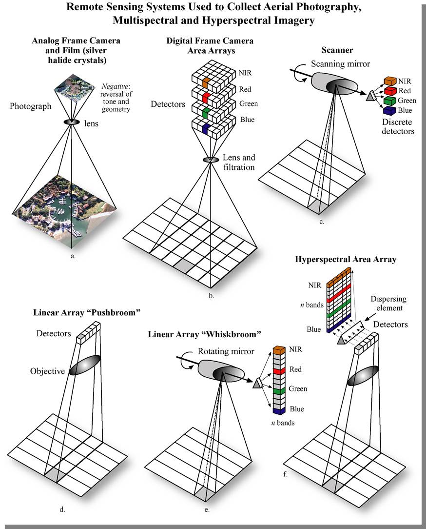
A linear array, or pushbroom scanner, is used in many spaceborne imaging systems, including SPOT, IRS, QuickBird, OrbView, and IKONOS. The position and orientation of the sensor are precisely tracked and recorded in the platform ephemeris. However, other geometric distortions, such as skew caused by the rotation of the earth, must be corrected before the imagery can be referenced to a ground coordinate system.
Several airborne systems, the Leica ADS-40 and the ITRES CASI, SASI, and TABI, also employ the pushbroom design. Each line of imagery is captured at a unique moment in time, corresponding with an instantaneous position and attitude of the aircraft. When direct georeferencing is integrated with these sensors, each single line of imagery has the exterior orientation parameters needed for rectification. However, without direct georeferencing, it is impossible to reconstruct the image geometry; the principles of space resection only apply to a rigid two-dimensional image.
The internal geometry of images captured by spaceborne scanning systems is much more complex. Across-track scanning and whiskbroom systems are more akin to a lidar scanner than to a digital area array imager. Each pixel is captured at a unique moment in time; the instantaneous position of the scanning device must also be factored into the image rectification. For this reason, a unique (and often proprietary) sensor model must be applied to construct a coherent two-dimensional image from millions of individual pixels. Add to this complexity the fact that there is actually a stack of recording elements, one for each spectral band, and that all must be precisely co-registered pixel-for-pixel to create a useful multiband image.
Direct georeferencing solves a large part of the image rectification problem, but not all of it. Remember, in our discussions of space resection and intersection, we learned that we can only extrapolate an accurate coordinate on the ground when we actually know where the ground is in relationship to the sensor and platform. We need some way to control the scale of the image. Either we need stereo pairs to generate intersecting light rays, or we need some known points on the ground. A georeferenced satellite image can be orthorectified if an appropriate elevation model is available. The effects of relief displacement are often less pronounced in satellite imagery than in aerial photography, due to the great distance between the sensor and the ground. It is not uncommon for scientists and image analysts to make use of satellite imagery that has been registered or rectified, but not orthorectified. If one is attempting to identify objects or detect change, the additional effort and expense of orthorectification may not be necessary. If precise distance or area measurements are to be made, or if the analysis results are to be used in further GIS analysis, then orthorectification may be important. It is important for the analyst to be aware of the effects of each form of georeferencing on the spatial accuracy of his/her analysis results and the implications of this spatial accuracy in the decision-making process.
Preprocessing
Defining characteristics of remote sensing instruments, platforms, and data were discussed in Lessons 1 and 2. Any remotely-sensed image or dataset can be defined in these terms and evaluated against the end-user application requirements to determine potential suitability. A raw scene can be produced in real-time or near-real-time from most digital sensors, and can be distributed as fast as the technology infrastructure allows. Simple visual interpretation can be quite useful for general situational awareness and decision-making. Most of us saw daily satellite images over the New Orleans Superdome after Hurricane Katrina and can appreciate the positive impact of these lightly-processed datasets.
Additional preparation and processing is often required for any more complex analysis. If the end-user application requires the overlay of multiple remotely sensed images or detailed GIS data, such as road centerlines and property boundaries, georeferencing must be performed. If spectral information is to be used to classify pixels or areas in the image based on their content, then the effects of the atmosphere must be accounted for. To detect change between multiple images, both georeferencing and atmospheric correction of all individual images may be required.
Georeferencing: The degree of accuracy and rigor required for the georeferencing depends on the desired accuracy of the result. More error can be tolerated in an image backdrop intended for visual interpretation, where a human interpreter can use judgment to work around some geographic misalignments. If the intent is to use automated processing to intersect, combine, or subtract one data layer from the other using mathematical algorithms, then the spatial overlay must be much more accurate in order to produce meaningful results. Higher accuracy is achieved only with better ground control, accurate elevation data, and thorough quality assurance. Most remotely-sensed data is delivered with some level of georeferencing information, which locates the image in a ground coordinate system. There are generally three levels of georeferencing, each corresponding to a different geometric accuracy.
- Level 1: uses positioning information obtained directly from the sensor and platform to roughly geolocate the remotely-sensed scene on the ground. This level of georeferencing is sufficient to provide geographic context and support visual interpretation of the data. It is not often not accurate enough to support robust image or GIS analysis that requires combining the remotely-sensed dataset with other layers.
- Level 2: uses a Digital Elevation Model (DEM) to remove relief displacement caused by variation in the height of the terrain. This improves the relative spatial accuracy of the data; distances measured between points within the geo-corrected image will be more accurate, particularly in scenes containing significant elevation changes. The DEM is usually obtained from another source, and the spatial accuracy of the Level 2 image will depend on the accuracy of the DEM.
- Level 3: uses a DEM and ground control points to most accurately georeferenced the image on the ground. In addition to the DEM, ground control points must be obtained from another source, and the accuracy of the Level 3 image will depend on the accuracy of the ground control points. Level 3 processing is usually required in order to provide the most accurate overlays of remotely-sensed data sets and other relevant GIS data.
Most satellite imagery is distributed with Level 1 georeferencing, which is often sufficient for making quick visual assessments of conditions on the ground. Additional processing to Level 2 or 3 (involving additional time and expense) is usually needed to analytically compare multiple scenes over the same location or precisely overlay other types of geographic information, such as property boundaries or building footprints. End-users may choose to perform this additional processing themselves, if they have the requisite control materials, expertise, and time.
Atmospheric Correction: If the end-user application intends to make use of spectral information contained in the image pixels to identify and separate different types of material or surfaces based on sample spectral libraries, then contributions to those pixels values made by the atmosphere must be removed. Atmospheric correction is a complex process utilizing control measurements, information about the atmospheric content, and assumptions about the uniformity of the atmosphere across the project area. The process is automated, but requires sophisticated software, highly skilled technicians, and again, time. Furthermore, atmospheric correction parameters used on one dataset cannot be summarily applied to a dataset collected on another day.
Image Interpretation
From a technology perspective, the simplest way to extract information from remotely sensed data is human interpretation. However, significant training and experience are needed to produce a skilled image interpreter. (Campbell, 2007) Eight elements of image interpretation employed by human image interpreters are:
- Image tone: the lightness or darkness of a region within an image.
- Image texture: the apparent roughness or smoothness of a region within an image.
- Shadow: may reveal information about the size and shape of an object which cannot be discerned from an overhead view alone.
- Pattern: the arrangement of individual objects in distinctive recurring patterns, such as buildings in an industrial complex or fruit trees in an orchard.
- Association: the occurrence of one type of object may infer the presence of another commonly associated object nearby.
- Shape: man made and natural features often have shapes so distinctive that this characteristic alone provides clear identification.
- Size: the relative size of an object related to other familiar objects gives the interpreter a sense of scale, which can aid in the recognition of objects less easily recognized.
- Site: refers to topographic position. For example, certain crops are commonly grown on hillsides or near large water bodies.
Tasks common to image interpretation are:
- Classification: assigning objects, features, or areas to classes. This occurs at three levels of confidence.
- Detection: determining the presence or absence of a feature.
- Recognition: assigning an object or feature to a general class or category.
- Identification: specifying the identity of an object with enough confidence to assign it to a very specific class.
- Enumeration: listing or counting discrete items visible on an image.
- Mensuration: measurement of objects and features in terms of distance, height, volume, or area.
- Delineation: drawing boundaries around distinct regions of the image characterized by specific tones or textures.
The results of image interpretation are most often delivered as a set of attributed points, lines, and/or polygons in any one of a variety of CAD or GIS data formats. The classification scheme or interpretation criteria must be agreed upon with the end user before the analysis begins.
Band Assignment
The interpretability of multispectral images can be improved through the spectral enhancement of the image. Such enhancements can either be temporary and reversible, or they can result in the creation of new data layers. Image enhancements that are commonly used to support the analysis of remotely sensed imagery.
Color Assignment for Computer Displays
By now, you should be familiar with the characteristics of the natural color image, the image which most closely resembles what you would expect to see looking down at earth from a plane. To create a natural color image, the spectral bands from the image are matched directly to the representative color display channels, or color guns, of the computer. For example, the red spectral band of a Landsat Image is matched to the Red color display channel on the computer, while the Green spectral band is matched to the Green color display and so on. In Figure 1.a, the natural colors of the scene provide adequate contrast between the urban areas and the forest; however, when compared to the other images in this figure, you will notice additional features that are not readily apparent in this natural color image. The reassignment of spectral bands to different color guns can improve the visibility of some image feature.
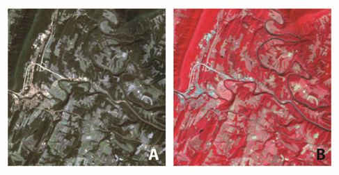
False-color-composite images are frequently used in remote sensing. The false-color-composite image is created by assigning spectral bands to color guns in combinations that do not create a natural color image. A common false-color-composite image used to support analysis of vegetation reassigns the near-infrared spectral band to the red color gun, the red spectral band to the green color gun, and the green spectral band to the blue color gun. The image that results from this combination is very different than the natural color image that you are used to seeing, as shown in Figure 1.b.
The major benefit of the false-color-composite is the increased ability to detect variations in vegetation due to the fact that vegetation strongly reflects NIR energy. In Figure 1.b, notice that it becomes easier to identify water features from the forested areas. In the natural color image, the lake in the lower left-hand corner blends in with the surrounding forest cover; the false-color-composite image highlights the lake's location. Fallow fields are evidenced by bright blue and white colors, while fields where crops have already grown are shown in the light pink angular patches that scatter across the darker red forests.
Band Math
The image enhancements that use the computer display to alter the appearance of an image are impermanent; they are usually saved only in the software project document. It is also possible to use mathematical and statistical methods to exploit relationships between spectral bands to create new archivable raster data products that can be also be interpreted. The Normalized Vegetation Difference Index (NDVI) is an example of such a product that is commonly used to support analysis of vegetation.
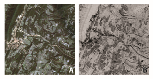
The calculation of NDVI is very straightforward. It is the ratio of the subtraction of the near-infrared and red bands to their sum [(NIR-RED)/(NIR+RED)], and its value ranges from -1 to 1, where green vegetation typically ranges between 0.2 and 0.9. In Figure 2, the NDVI image is useful for identifying agricultural fields that are in different phases of growth. Fallow fields here are dark, having low NDVI values, while green vegetation, such as the forests on the ridgeline, are much brighter. The NDVI image emphasizes the location of water bodies and impervious surfaces (black), but does a poor job of differentiating between the two based on value alone. Instead, the visual interpretation element of shape can be used to differentiate here the meandering river and the relatively straight roadway.
More sophisticated methods of analyzing spectral data also exist. The Tasseled-Cap Transformation is a statistical method for reducing multispectral data. First designed to support agricultural analysis (Kauth and Thomas 1976), it has also been shown to be useful in land cover change mapping (Healey et al. 2005). Like NDVI described above, this transformation takes advantage of the differences in NIR and RED reflectance.
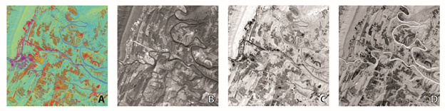
The Tasseled-Cap Transformation decomposes a multispectral image into three main components that comprise 97% of the Landsat spectral data content; these components are brightness, greenness, and wetness. Each is said to be related to particular physical feature types:
- Brightness, Figure 2B, is assigned to the Red color display channel is associated with impervious surfaces such as asphalt.
- Greenness, Figure 2C, is assigned to the Green color display, is associated with vegetation.
- Wetness, Figure 2D, is assigned to the Blue color display, is associated with moisture.
Each of the three components can be visualized separately; however, when combined, these three components can provide great insights into the landscape as shown in Figure 2A. This Tasseled-Cap Color image highlights differences between features that are not found by looking at the NDVI image. For example, it is possible to identify a road feature by its thin linear shape and low reflectance values in the NDVI image. Looking at that same feature, Tasseled-Cap Color image, reveals more subtle differences. Look at the small built-up area in the left of the images. In the NDVI image, this feature looks to be one feature, however, looking at the Tasseled-Cap image we can see that what seemed to be a single feature really is many smaller features.
You have now looked at several methods for enhancing the spectral data from remotely sensed images. In order to maximize the usefulness of such transformations, an analyst must choose the enhancement most appropriate to the task at hand. Spectral enhancements alone are not enough on their own to make interpretation accurate; a good command of the various interpretation elements, combined with strong contextual knowledge of the image under analysis, contributes to successful interpretation.
Healey, S. P., W. B. Cohen, Y. Zhiqiang & O. N. Krankina (2005) Comparison of Tasseled Cap-based Landsat data structures for use in forest disturbance detection. Remote Sensing of Environment, 97, 301-310.
Kauth, R. J. & G. Thomas. 1976. The tasseled cap--a graphic description of the spectral-temporal development of agricultural crops as seen by Landsat. In LARS Symposia, 159.
Digital Image Classification
Digital image classification uses the quantitative spectral information contained in an image, which is related to the composition or condition of the target surface. Image analysis can be performed on multispectral as well as hyperspectral imagery. It requires an understanding of the way materials and objects of interest on the earth's surface absorb, reflect, and emit radiation in the visible, near-infrared, and thermal portions of the electromagnetic spectrum. In order to make use of image analysis results in a GIS environment, the source image should be orthorectified so that the final image analysis product, whatever its format, can be overlaid with other imagery, terrain data, and other geographic data layers. Classification results are initially in raster format, but they may be generalized to polygons with further processing. There are several core principles of image analysis that pertain specifically to the extraction of information and features from remotely sensed data.
- Spectral differentiation is based on the principle that objects of different composition or condition appear as different colors in a multispectral or hyperspectral image. For example, a newly planted cornfield has a distinct color when compared to a field of mature plants, and yet another color when the field has been harvested. Corn has a distinct color as compared to wheat; healthy plants are a different color than pest-infested or drought-impacted plants. The use of spectral signature, or color, to distinguish types of ground cover or objects is called spectral differentiation.
- Radiometric differentiation is the detection of differences in brightness, which may in certain cases be used to inform the image analyst as to the nature or condition of the remotely sensed object.
- Spatial differentiation is related to the concept of spatial resolution. We may be able to analyze the spectral content of a particular pixel or group of pixels in a digital image when those pixels comprise a single homogeneous material or object. It is also important to understand the potential for mixing of the spectral signatures of multiple objects into the recorded spectral values for a single pixel. When designing an image analysis task, it is important to consider the size of the objects to be discovered or studied compared to the ground sample distance of the sensor.
The extraction of information from remotely sensed data is frequently accomplished using statistical pattern recognition; land-use/land-cover classification is one of the most frequently used analysis methods (Jensen, 2005). Land cover refers to the physical material present on the earth’s surface; land use refers to the type of development and activities people undertake in a particular location. The designation of “woodland” for a tree-covered area is a land cover classification; the same woodland might be designated as “recreation area” in a land use classification.
While certain aspects of digital image classification are completely automated, a human image analyst must provide significant input. There are two basic approaches to classification, supervised and unsupervised, and the type and amount of human interaction differs depending on the approach chosen.
- Supervised classification requires the image analyst to choose an appropriate classification scheme, and then identifies training sites in the imagery that best represent each class. A simple land cover classification scheme might consist of a small number of classes, such as urban, water, wetlands, forest, grass/crops. Individual sites that fall into a single class may have slightly different spectral characteristics; for example, the spectral signature of a water body will depend on the amount of suspended sediment or plant material in the water. Urban land cover signatures will vary based on the type of materials used; asphalt has a very different spectral signature from concrete, wood, or glass. The image analyst must select a sufficient number of training sites in each class to represent the variation present within each class in the image. The classification algorithm then uses spectral characteristics of the training sites to classify the remainder of the image. Training sites developed in one scene may or may not be transferrable to an entire study area. If ground conditions, lighting conditions, or atmospheric effects change from scene to another, then training sites must be developed independently for each scene. Furthermore, training sites may not be transferrable across time; in addition to the conditions noted above that change over time as well as space, real changes in the land cover occurring at a training site location over time will cause incorrect classification results in the second image. Accurate supervised classification results depend entirely on the analyst’s ability to collect a sufficient number of training sites and to recognize when training sites can or cannot be transferred from one image to another.
- Unsupervised classification requires less input from the analyst before processing. The classification algorithm searches and analyzes the image, grouping pixels into clusters which it deemed to be uniquely representative of the image content. After classification, the image analyst must determine if these arbitrary classes have meaning in the context of the end-user application. A significant amount of time may be spent trying to determine the physical meaning of a class identified by the unsupervised algorithm. In addition, experimentation is required to determine the optimal number of unique classes used for initialization of the algorithm. Furthermore, there is no basis to believe that the classes discovered in one image will be the same classes discovered in a second image. Time spent trying to optimize and interpret the unsupervised results may far exceed the time an analyst would have spent selecting training sites for supervised classification. Finally, because it is impossible to ensure consistency in class identification from one image to the next, unsupervised classification is not useful for change detection.
Classification schemes may be comprised of hard, discrete categories; in other words, each pixel is assigned to one, and only one, class. Fuzzy classification schemes allow a proportional assignment of multiple classes to pixels. The entire image scene may be processed pixel-by-pixel, or the image may be decomposed into homogeneous image patches for object-oriented classification. As stated by Jensen (2005), “no pattern classification method is inherently superior to any other.” It is up to the analyst, using his/her knowledge of the problem set, the study area, the data sources, and the intended use of the results, to determine the most appropriate, efficient, time and cost-effective approach.
Measuring the accuracy of classification requires either comparison with ground truth or comparison with an independent result. Errors of omission are committed when an object is left out of its true class (a tree stand which is not classified as forest, for example); errors of commission are committed when an object that does not belong in a class is incorrectly included (in the example above, the tree stand is incorrectly classified as a wetland).