Lesson 4 Object-Oriented Programming in Python and QGIS Development
4.1 Overview and Checklist
This lesson is two weeks in length. The focus will be on diving into the object-oriented programming aspects of Python and you will finally learn how to define your own classes in Python as well as derive new classes as subclasses of already existing classes. We will also return to the topic of GUI development and apply what we learned on object-oriented programming to create a standalone application and (optionally) plugin for the open-source GIS software QGIS. To prepare for that, the lesson starts with a theoretical section on Python collections, followed by an introduction to QGIS and its Python API.
After the end of the first week, you are supposed to submit a proposal for a term project. Please refer to the Calendar for specific time frames and due dates. To finish this lesson, you must complete the activities listed below. You may find it useful to print this page first so that you can follow along with the directions.
| Step | Activity | Access/Directions |
|---|---|---|
| 1 | Engage with Lesson 4 Content | Begin with 4.2 Collections and Sorting |
| 2 | Term project proposal | Submit your term project proposal by the end of the first week of the lesson |
| 3 | Programming Assignment and Reflection |
Submit your code for the programming assignment and 400 words write-up with reflections |
| 4 | Quiz 4 | Complete the Lesson 4 Quiz |
| 5 | Questions/Comments | Remember to visit the Lesson 4 Discussion Forum to post/answer any questions or comments pertaining to Lesson 4 |
4.2 Collections and Sorting
In programming, you are often dealing with collections of items of the same data type, e.g. collections of integer numbers, collections of Point objects, etc. You are already familiar with the built-in collection types list, tuple, and dictionary, but there exist more data structures for storing collections of items. Which data structure is best suited for a specific task depends on what operations exactly you need to perform with the data structure and items in it. For instance, a dictionary is the right choice if you mainly need to access the stored items based on their key. In contrast, a list is a good choice if you have a static collection of items that you need to iterate over or that you want to access based on their index. In general, there often exist several collection data types that you can use for a given task but some of them will be more efficient and better choices than the others.
Here is a little introductory example:
Let’s say that, in your Python program, you have different assignments or jobs coming in that need to be performed in the order in which they arrive. Since performing an assignment can take some time, you need to store the assignments in some sort of waiting queue: the next assignment to be performed is always taken from the front of the queue, while the new assignments arriving are added at the end of the queue. This approach is often referred to as the first-in-first-out (FIFO) approach.
To implement the waiting queue in this program, we could use a normal list. New assignments are added to the end of the list with list method append(), while items can be removed at the beginning of the list by calling the list method pop(...) with parameter 0. The following code simulates the arriving of new assignments and removing of the next assignment to be performed, starting with a queue with three assignments in it. For simplicity we alternate between an assignment being removed and a new assignment arriving, meaning the queue will always contain two or three assignments. We also simply use strings with an increasing number at the end for the assignments, while in a real application these would be more complex objects with attributes describing the assignment.
waitingQueue = ["Assignment 1", "Assignment 2", "Assignment 3"]

for count in range(3,100001):
	waitingQueue.pop(0)                             # remove assignment at the beginning of the list/queue
	waitingQueue.append("Assignment " + str(count)) # add new assignment at the end of the list/queue
Run this program with basic code profiling as explained in Section 1.7.2.1. One thing you should see in the profiling results is that while the Python list implementation is able to perform append operations (adding at the end of the list) rather efficiently, it is not particularly well suited for removing (and also adding) elements at the beginning. There exist data structures that are much better suited for this task as the following version shows. It uses the collection class deque (standing for “double-ended queue”) that is defined in the collections module of the Python standard library, which contains several specialized collection data structures. Deque is optimized for adding and removing elements at the start and end of the collection.
import collections

waitingQueue = collections.deque(["Assignment 1", "Assignment 2", "Assignment 3"])

for count in range(3,100001):
	waitingQueue.popleft()                          # remove assignment at the beginning of the deque
	waitingQueue.append("Assignment " + str(count)) # add new assignment at the end of the deque
Please note that the deque method for removing the first element from the queue is called popleft(), while pop() removes the last element. The method append() adds an element at the end, while appendleft() adds an element at the start (we don’t need pop() and appendleft() in this example). The initial deque is created by giving the list of three assignments as a parameter to collections.deque(...).
If you profile this second version and compare the results with those of the first version using a list, you should see that deque is by far the better choice for implementing this kind of waiting queue. More precisely, adding elements at the end takes about the same time as for lists but removing elements at the front is approximately three times as fast (and as fast as adding at the end).
While we cannot go into the implementation details of lists and deque here (you may want to check out a book on algorithms and data structures in Python to learn how to implement such collections yourself), hopefully this example makes it clear that it’s a good idea to have some understanding of what collection data structure are available and which operations are fast with them and which are slow.
In the following, we are going to take a quick look at sets and priority queues (or heaps) as two examples of other specialized Python collections, and we talk about the common operation of sorting collections.
4.2.1 Sets
Sets are another built-in collection in Python in addition to lists, tuples, and dictionaries. The idea is that of a mathematical set, meaning that there is no order between the elements and an element can only be contained in a set once (in contrast to lists). Sets are mutable like lists or dictionaries.
The following code example shows how we can create a set using curly brackets {…} to delimit the elements (similar to a dictionary but without the
s = {3,4,1,3,4,1} # create set
print(s)
Output:
{1, 3, 4}
Since sets are unordered, it is not possible to access their elements via an index but we can use the “in” operator to test whether or not a set contains an element as well as use a for-loop to iterate through the elements:
x = 3
if x in s:
     print("already contained")

for e in s:
    print(e)
Output:
already contained
1
3
4
One of the nice things about sets is that they provide the standard set theoretical operations union, intersection, etc. as shown in the following code example:
group1 = { "Jim", "Maria", "Frank", "Susan"}
group2 = { "Sam", "Steve", "Jim" }

print( group1 | group2 )  # or group1.union(group2)

print( group1 & group2 )  # or group1.intersection(group2)

print( group1 - group2 )  # or group1.difference(group2)

print( group1 ^ group2 )  # or group1.symmetric_difference(group2)
Output:
{'Frank', 'Sam', 'Steve', 'Susan', 'Maria', 'Jim'}
{'Jim'}
{'Susan', 'Frank', 'Maria'}
{'Frank', 'Sam', 'Steve', 'Susan', 'Maria'}
The difference between the last and second-to-last operation here is that group1 - group2 returns the elements of the set in group1 that are not also elements of group2, while the symmetric difference operation group1 ^ group2 returns a set with all elements that are only contained in one of the groups but not in both.
4.2.2 Sorting
One common operation on collections is sorting the elements in a collection. Python provides a function sorted(…) to sort the elements in a collection that allows for iterating over the elements (e.g. a list, tuple, or dictionary). The result is always a list. Here are two examples:
l1 = [9,3,5,1,-2]
print(sorted(l1))

l2 = ("Maria", "Frank", "Sam", "Mike")
print(sorted(l2))
Output:
[-2, 1, 3, 6, 9]
['Frank', 'Maria', 'Mike', 'Sam']
If our collection is a list, we can also use the list method sort() instead of the function sorted(…), e.g. l1.sort() instead of sorted(l1) . Both work exactly the same.
sorted(…) and sort() by default sort the elements in ascending order based on the < comparison operator. This means numbers are sorted in increasing order and strings are sorted in lexicographical order [1]. When we define our own classes (Section 4.6) and want to be able to sort objects of a class based on their properties, we have to define the < operator in a suitable way in the class definition.
The keyword argument ‘reverse’ can be used to sort the elements in descending order instead:
print( sorted(l2, reverse = True) )
Output:

['Sam', 'Mike', 'Maria', 'Frank']
In addition, we can use the keyword argument ‘key’ to provide a function that will be applied to the elements and they will then be sorted based on the values returned by this function. For instance, the following example uses a lambda expression for the ‘key’ parameter to sort the names from l2 based on their length (in descending order) rather than based on their lexicographical order:
print( sorted(l2, reverse = True, key = lambda x: len(x)) )
Output:

['Maria', 'Frank', 'Mike', 'Sam']
Sorting can be a somewhat time-consuming operation for larger collections. Therefore, if you mainly need to access the elements in a collection in a specific order based on their properties (e.g. always the element with the lowest value for a certain attribute), it is advantageous to use a specialized data structure that keeps the collection sorted whenever an element is added or removed. This can save a lot of time compared to frequently re-sorting the collection. An example of such a data structure is the so-called priority queue or heap. The heapq module of the Python standard library implements an algorithm for realizing a priority queue in a Python list and we are going to discuss it in the final part of this section.
4.2.3 Priority Queues and Heapq
The idea of a priority queue is that items in the collection are always kept ordered based on their < relation so that when we take the first item from the queue it will always be the one with lowest (or highest) value.
For instance, let’s get back to the example we started this section with of managing a queue of assignments or tasks that need to be performed. Let’s say that instead of performing the assignments in the order in which they arrive (first-in-first-out), the assignments have a priority value between 1 and 9 with 1 meaning highest and 9 meaning lowest priority. That means we need to make sure we keep the assignments in the queue ordered based on their priority so that taking the first assignment from the queue will be that with the highest priority.
The heapq module among other things provides a set of functions for adding elements to a list (function heappush(…)) and for removing the first item with highest priority (function heappop(…)). In the following code, we again use strings for representing our assignments and encode the priority in the strings themselves so that their lexicographical order corresponds to their priority, i.e. “Assignment 1” < “Assignment 2” < … < “Assignment 9”. The reason we defined the highest priority to be given by the number 1 and the lowest priority by the number 9 is that heapq implements a min heap in which heappop(…) always returns the lowest value element according to the < relation in contrast to a max heap in which heappop(…) would always return the highest value element. The code starts with an empty list in variable pQueue and then simulates the arrival of 100 assignments with random priority using heappush(…) to add a new assignment to the queue.
import heapq
import random

pQueue = []

for count in range(1,101):
    priority = random.randint(1,9)
    heapq.heappush(pQueue, 'Assignment ' + str(priority))

print(pQueue)
When you look at the output produced by the print statement in the last line, you may be disappointed because it doesn’t look like the list is really ordered based on the priority numbers of the assignments. However, the list also does not reflect the order in which the assignments have been added to the queue. The list is actually a “flattened” representation of a binary tree [2], the data structure that heapq is using to make the push and pop operations as efficient as possible, while making sure that heappop(…) always gives you the lowest value element from the queue.
Now add the following code that calls heappop(…) 100 times to remove all assignments from the queue and print out their names including their priority value:
for count in range(1,101):
    assignment = heapq.heappop(pQueue)
    print(assignment)
Output:

Assignment 1
Assignment 1
…
Assignment 2
…
Assignment 9
As you can see, by using heappop(…) we indeed get the assignments in the right order from the queue. Of course, this is a simplified example in which we first fill the queue completely and then empty it again, but it works in the same way if we add and remove assignments in any arbitrary order. Using heapq for this task is much, much faster than any simple approach such as always searching through the entire list to find the element with the lowest value or, slightly better, always searching for the correct position when inserting a new assignment into the list to keep the list sorted. If you don't believe it, try to implement your own method and do some profiling to see how it compares to the priority queue based approach.
In the walkthrough of this lesson, we will employ this notion of a priority queue for keeping a number of bus track GPS observations sorted based on their timestamps. For this, we will have to define the < method for our observation points in a suitable way to work with heapq. This will allow us to process the observation points in chronological order.
This section gave you a bit of a taste of the idea of efficient data structures for collections, the algorithms behind them, and the trade-offs involved (a data structure that is very efficient for certain operations will be suboptimal for other operations). Computer science students spend a lot of time studying the implementation and properties of such data structures and the time and space complexities [3] of the operations involved. We were only able to scratch the surface of this topic here, but, as indicated above, there are many books and other resources on this topic, including some specifically written for Python.
4.3 Open source desktop GIS software
While in lessons 1 and 2 we mainly focused on advanced Python programming approaches within the ESRI ArcGIS world, lesson 3 involved a step away from proprietary GIS software towards open source Python libraries and software tools, even though one of the main points we wanted to make in this lesson was that both worlds are not as separated as one might think. In this final lesson of the course, we will be leaving ArcGIS behind completely and take a closer look at the open source alternative QGIS, a free desktop GIS that most likely you have already heard of.
While the history of open source GIS software goes back more than 30 years, open source desktop GIS software has only very recently reached a level of maturity and intuitive usability that can be considered comparable to proprietary desktop GIS software. With desktop GIS software we mean standalone software that can be installed and run locally on a computer and that makes the most common GIS data manipulation and analysis functionalities (for at least both raster and vector data) accessible via an easy-to-use GUI, similar to the ArcGIS Desktop products. However, these days there do exist multiple such open source alternatives, including the ones we briefly list below:
Grass GIS
Grass (Geographic Resources Analysis Support System) [4] is the ancestor of open source GIS but is still under active development, with a history of more than 30 years. Its development was started by the U.S. Army Construction Engineering Research Laboratories in 1982 but it is now maintained by the Open Source Geospatial Foundation [5] (OSGeo) under GNU GPL license. Grass is largely written in C/C++ and provides a large collection of GIS tools grouped into modules. Other open source GIS systems, such as QGIS for example, integrate these GRASS modules to extend their functionality.
gvSIG Desktop
gvSIG Desktop [6] is a much younger open source software by gvSIG Association written in Java. Its initial release was in 2004. Similar to Grass, it is published under the GNU GPL license. The most recent version (at the time of this writing) is 2.5.1 released in March 2020.
MapWindow GIS
MapWindow [7] is an open source project that, in contrast to most of the others listed here, is only available on Windows. It is written in C# for the .NET platform, available under the Mozilla Public License, and maintained and updated by a team of volunteers. MapWindow is available in version 4. In 2015, a complete rewrite of the software was started that is currently available as MapWindow5 version 5.2.0.
OpenJump
OpenJump [8], originally called Jump GIS and designed by Vivid Solutions, is another Java based open source GIS software developed by a team of volunteers. Like most other GIS systems, it provides an interface for creating plugins to extend its functionality. The latest release, version 2.2.1, is from the May 2023. OpenJump is published under GNU GPL license.
SPRING
SPRING [9] is a freeware GIS and one of the older GIS systems available. It is developed by the Brazilian National Institute for Space Research (INPE) since 1992. In particular, it provides advanced remote sensing data and image processing capabilities. SPRING requires you to register before being able to acquire the software and has a special license specifying how it can be used.
uDig
uDig [10] is a Java-based GIS system that is embedded into the Eclipse platform. It is developed by Refractions Research and published under Eclipse Public License EPL. Currently, the newest available version is the release candidate for version 2.2.
QGIS
Lastly, we come to QGIS [11], the open source software that this lesson will mainly be about. Development of QGIS was started in 2002 by Gary Sherman under the name Quantum GIS. QGIS publishes updates in short intervals and a new milestone has been reached with the release of version 3.0 in February 2018. QGIS is by many considered to be the leading open-source desktop GIS software due to the broad range of functionality it provides, its easy-to-use and flexible interface, and the very active community. QGIS has been written in C++ and Python. It provides an interface for extending its capabilities via plugins written in Python that we will work with later on in this lesson. QGIS is developed by a team of volunteers and organizations, and supported by the Open Source Geospatial Foundation [12] umbrella organization for open source GIS software. It is published under GNU GPL license.
From a programming perspective, the focus of this lesson will be on object-oriented programming in Python with the goal of gaining a better understanding of some concepts like objects and classes that we have already been using quite a lot in Geog485 and in the first lessons of this course. But now we will study this topic in more depth and you will learn how to write your own classes and use them effectively in your own programming projects to produce better-structured code that is also more readable and easier to maintain. You will apply what you learned theoretically in this lesson to write plugins for QGIS to extend its capabilities. Implementing these plugins will also include further GUI designing work with QT as a continuation of what you learned in lesson 2. However, before we further talk about object-oriented programming, we provide a brief overview on QGIS in the next section.4.4 QGIS: A Brief Overview
QGIS follows a very rigorous release schedule in which new versions are released every three months and each 4th release is a so-called long-term release (LTR) that will be maintained for a full year (see the release schedule [13]). Not too long ago, QGIS made a big step forward with the release of version 3.0 in February 2018. This was the first version based on Python 3 (not Python 2 anymore) and whose GUI was based on QT5 (not QT4 anymore). In this section, you will be downloading and installing QGIS on your computer and then familiarizing yourself with its graphical interface which has quite a lot in common with ArcGIS but also has some components that work a bit differently, such as the map composer part of the software.
In case you have already worked with QGIS in the past, it is still important that you make sure you have version 3 (or higher) of QGIS installed on your computer using the approach described in the following because of the switch to Python 3 and QT5 mentioned above and because the development we are going to do will require some further components to be installed. While there are some changes in the interface from version 2.18 to version 3, you can probably go through the familiarization part rather quickly if you have worked with QGIS 2 (or a previous version of QGIS 3) before.
4.4.1 Downloading and installing QGIS
In this section, we will provide instructions for installing QGIS via the OSGeo4W distribution manager and for setting up your system to be prepared for the QGIS programming work, we are going to do in this lesson. The OSGeo4W/QGIS installation includes its own Python 3 environment and you will have make sure that you use this Python installation for running the qgis based examples from the later sections. One way to achieve this is by executing the scripts via commands in the OSGeo4W shell, after executing some commands that make sure that all environment variables are set up correctly. This will also be explained below.
OSGeo4W and QGIS installation
To install the OSGeo4W environment with QGIS 3.x, please follow the steps below:
- Go to the qgis website [11]
- Click "Download now"
- Pick the Windows "OSGeo4W Network Installer" close to the top (not the green button for the standalone installer!)
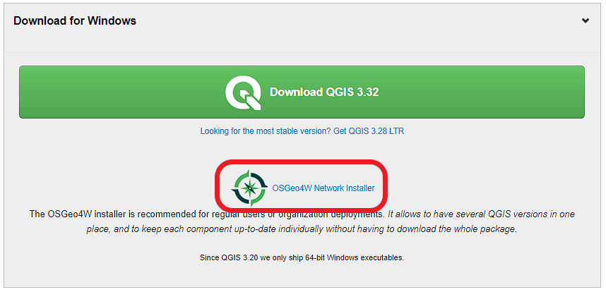 Figure 4.1 Downloading the OSGeo4W installer
 - Click on the link that says "Download OSGeo4W Installer and start it" to downloaded a file called osgeo4w-setup.exe . Then run that file to start the installation.
- Select the "Express Desktop Install" option (Unless you already have OSGeo4W/QGIS installed, then use the Advanced option to ensure you get the latest versions of all packages/tools or pick a different installation folder. If you get errors attempting to run QGIS, you may have to delete your c:\OSGEO4W folder and re-run the installation.)
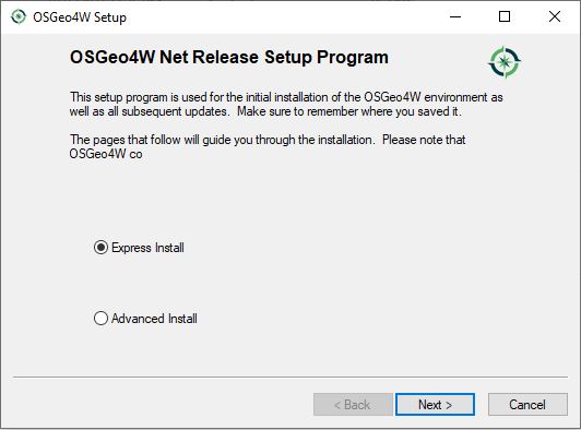 Figure 4.2 Selecting the Express Desktop Install option
 - If asked, select a site from which to install (does not matter which)
- When asked which packages to install, select the options shown in the screenshot below. Apart from that you can accept the default settings on the next pages.
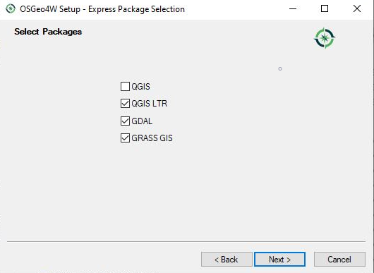 Figure 4.2b Selecting the packages to install
 - Accept the different licenses and run the installation (ignore warnings about corrupted packages if you get them and just click 'Next' if you get warnings about missing dependencies)
Where to find what?
After the installation has finished, you should have a folder called OSGeo4W in the root folder of your C: drive (unless you picked a different folder for the installation). Here we list the main programs from this installation folder that you will need in this lesson:
- C:\OSGeo4W\OSGeo4W.bat - This opens the OSGeo4W shell that can be used for executing python scripts from the command line.
- C:\OSGeo4W\bin\qgis-ltr-bin.exe - This is the main QGIS executable that you need to run for starting QGIS 3.
- C:\OSGeo4W\apps\Qt5\bin\designer.exe - This is the QT Designer executable that you can use for creating Qt5 GUIs in this lesson. If you simply double-click the .exe file in the Windows File Explorer, you will most likely get an DLL related error message because some environment variables won't be set correctly. But you should be able to run the program by opening the OSGeo4W shell and typing the command designer there.
- python-qgis-ltr - As explained further below, you can use this command in the OSGeo4W shell for setting the path and environment variables for running qgis and PyQT5 based Python 3 code as well as executing scripts directly.
Running OSGeo4W shell and commands for qgis and PyQt5 development
When you run OSGeo4W.bat, the OSGeo4W shell will show up looking similar to the normal Windows command line but providing some additional commands that can be listed by typing in "o-help".
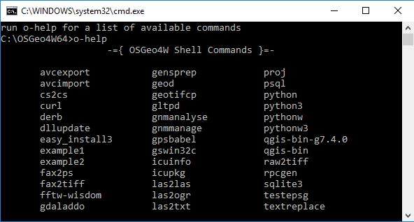
When using the OSGeo4W shell in this lesson, it is best to always execute the command
python-qgis-ltr
first to make sure all environment variables are set up correctly for running qgis and PyQt5 based Python code. The command will start a Python interpreter (recongnizable by the >>> prompt) that you can immediately leave again by typing the command quit() . You can also directly run Python scripts with python-qgis-ltr by writing
python-qgis-ltr xyz.py
rather than just
python xyz.py
You can also use the command pyrcc5 in the OSGeo4W shell for compiling QT5 resource files that we will need later on in this lesson.
Installing geopy package and pandas
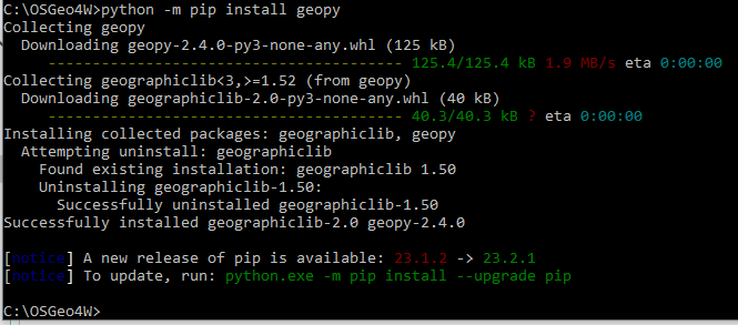
Most of the Python packages we will need in this lesson (like PyQt5) are already installed in the Python environment that comes with OSGeo4W/QGIS, but a few additional pieces are necessary. There is one package that we will use for performing distance calculations between WGS84 points in the two walkthroughs of the lesson. The package is called geopy and it needs to be installed first. To do this, please open the OSGeo4W shell and change to Python 3 by running the python-qgis-ltr command followed by quit() as described above, and then run the following pip installation command:
python -m pip install geopy
The package is small, so the installation should only take a couple of seconds. The output you are getting may look slightly different than what is shown in the image below but should indicate that geopy has been installed successfully.
In the practice exercise for this lesson, we will also use pandas. In earlier versions of QGIS/OSGeo4W, pandas wasn't installed by default. To make sure, simply run the following command for installing pandas; most likely it's going to tell you that pandas is already installed:
python -m pip install pandas
Installing the required QGIS plugins
We will need a few QGIS plugins in this lesson, so let's install those as well. Some of these are for the optional part at the end but they are small and installation should be quick, so let's install all of them now. Please follow the instructions below for this:
- Start QGIS
- Go to Plugins -> Manage and Install Plugins in the main menu bar
- Under "Settings", make sure the box next to "Show also experimental plugins" is checked.
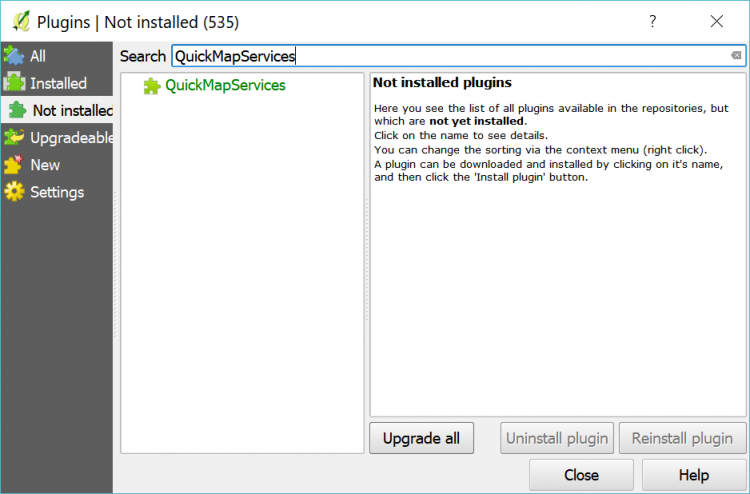
- Under "Not installed" look for the following three plugins and install them:
- QuickMapServices (allows for quickly adding basemaps like OSM to a project)
- Plugin Builder 3 (for creating templates for new plugins)
- Plugin Reloader (for reloading a plugin after modifying the code)
If you now click on "Installed", all three plugins should appear in the list of installed plugins with a checkmark on the left, which indicates that the plugin is activated.
4.4.2 Familiarizing yourself with QGIS
Important note: This lesson has a lot of content and this is one of its less important sections. We included it so that, if you have not worked with QGIS before, you get an idea of where to find what and how things work in QGIS in general. However, since we will mainly be using the QGIS programming API rather than doing things in QGIS itself, we recommend that you go through this section quickly and then maybe come back at the end of the lesson if you have an interest in learning more about QGIS and its interface.
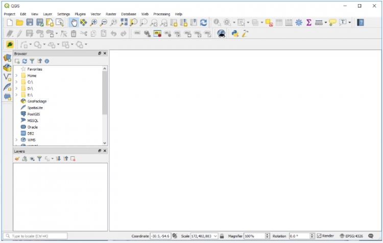
When you open QGIS 3 for the first time, it will look similar to the image below. The main elements are the main menu bar at the top, a number of horizontal toolbars with buttons for different operations below the menu bar, a smaller vertical toolbar on the left side with buttons for adding or creating layers, and then three main windows: a panel with a file browser, a panel that lists the layers in your project (currently empty), and then the main window for displaying the current project. At the very bottom, you can find a status bar displaying information related to the project window such as the scale and coordinate reference system used. Overall, this all looks somewhat similar to ArcGIS Desktop or Pro. All toolbars and panels can be freely moved around, undocked and docked back again, and there are many additional panels and toolbars that can be enabled/disabled either from the main menu under View -> Panels/Toolbars or by doing a right-click on one of the panel title bars or toolbar areas at the top and left.
There are several ways to add a data set to a project:
- By navigating to a file in the file browser panel and then double-clicking it.
- By dragging a file from the Windows File Explorer onto the project window or layers panel.
- By clicking the “Open Data Source Manager”
 button, which will open up a dialog with a list of different types of sources on the left including local files, datasets from different databases, and also data sets provided as web services (WMS, WFS, ArcGIS Map Server or Feature Server, etc.).
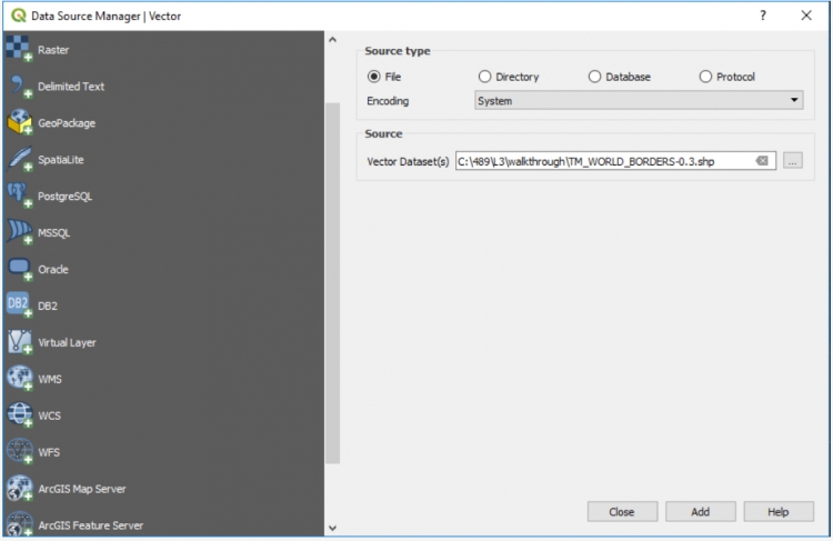
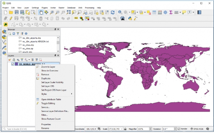
Feel free to try out adding different data sets to the project. Similar to ArcGIS, the coordinate reference system used for the project and project window will be that of the first source added, but of course this can be changed, e.g. by going Project -> Project Properties…. in the menu bar or by left-clicking the CRS field in the status bar. Dragging the layers and the buttons at the top of the Layers panel can be used to arrange the layers in a certain order and group or filter them. We here add the world borders layer from Lesson 3 to the project. The layer now shows up in the project window and the Layers panel. Right-clicking the layer in the Layers panel will provide a number of options for that layer. Double-clicking the layer will directly open the “Layer Properties” dialog with a lot of options to change rendering or other properties of the layer.
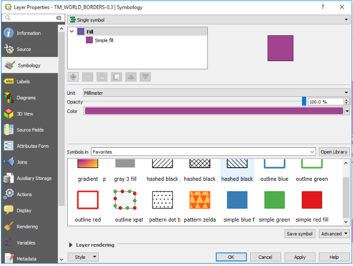
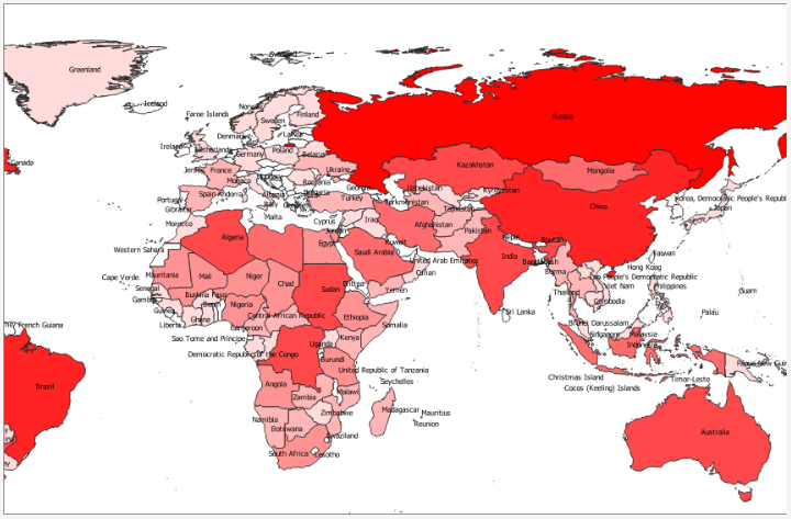
The properties you will most commonly work with are the Symbology and Labels properties. When coming from ArcGIS, working with these dialogs requires a bit of getting used to. Give it a try by attempting to show the world borders layer with a Graduated scheme based on the “AREA” attribute of the layer using a Natural Breaks classification with 8 classes and with labels based on the “NAME” attribute. The result should look somewhat similar to the image below. If you have any problems achieving this, please post on the Lesson 4 discussion forum.
If you want to select features from a layer based on attribute, the Query Builder dialog can be opened by doing a right-click -> Filter … on the layer in the Layers panel. The dialog itself works roughly similar to the corresponding component of ArcGIS. You can check out the attribute table of the layer by doing a right-click -> Open Attribute Table. Working with the attribute table again is roughly similar to ArcGIS. If you want to export a layer as a new data set, you do a right-click -> Export -> Save Features as… . This, for instance, allows for saving only the currently selected features and/or saving the layer in a different format or using a different CRS.
Looking at the main menu bar, we find the main tools for working with Vector and Raster data under the respective submenus. They include typical geoprocessing, data manipulation, and analysis tools. Additional tools can be accessed by opening the Processing Toolbox panel under Processing -> Toolbox. Moreover, QGIS has a plugin interface that allows for writing extensions to QGIS. Plugins can be managed and new plugins can be installed under Plugins -> Manage and Install Plugins, and they can add new entries to menu bar and tool bars. QGIS plugins are written in Python, and you will learn how to do so later on in this lesson. QGIS also has a Python Console (Plugins -> Python Console) that allows for entering and executing Python code that uses the QGIS Python API.
A QGIS project is saved as a .qgz file using Project -> Save or Project -> Save As…. From this menu, you can also open a new project, export the project map in different formats, etc.
One thing that works a bit differently than in ArcGIS is the layout composer component for creating map views of your project including additional elements such as a legend, scale bar, etc. By going Project -> New Print Layout, you can create a new map layout document. This opens up a new window with its own interface that allows you to arrange maps and other elements like images and text in the same way as in a vector graphics or publishing tool. The created layout can just be a single page or span multiple pages and contain different maps. Elements are added to the page with the buttons from the toolbar on the left. A list of all elements is shown in the panel on the top right. The properties of the currently selected element can be accessed and changed with the panel on the bottom right. The simple layout in the image below was created by adding our current map with the add map  button, adding a text element with the add text button
  , and then adding a legend for the current map with the add legend
  button.
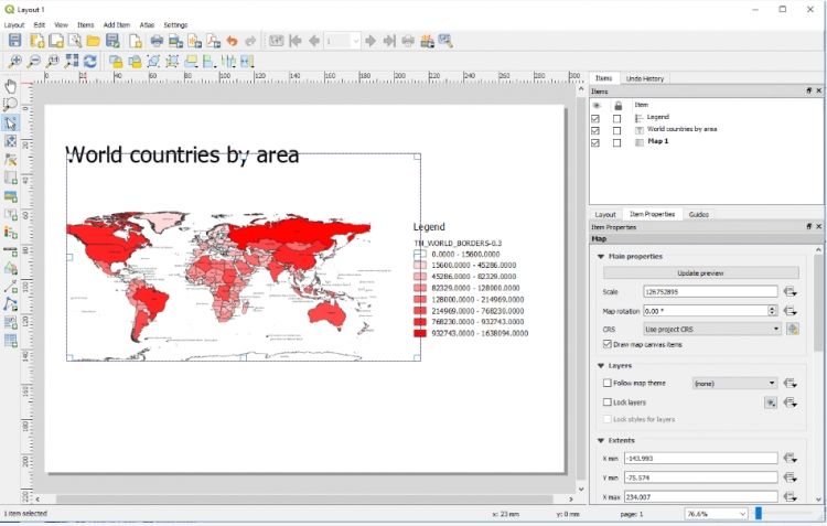
Layouts can be exported as images or PDF files and previously created layouts can be accessed via the Layout Manager under Project -> Layout Manager… or directly be accessed from Project -> Layouts -> … .
This short overview should be enough to get you started but, of course, only covers the basics. This lesson will focus on the QGIS Python API and using it to write programs or plugins for QGIS, rather than on working with the QGIS interface directly. Nevertheless, if you want to learn more about QGIS at some point, the following tutorials covering certain tasks in more detail can be used as a starting point.
- Making a map [14]
- Working with attributes [15]
- Basic vector styling [16]
- Raster styling and analysis [17]
More tutorials are available at this QGIS Tutorials and Tips page [18].
4.5 The QGIS Scripting Interface and Python API
QGIS has a Python programming interface that allows for extending its functionality and for writing scripts that automate QGIS based workflows either inside QGIS or as standalone applications. The Python package that provides this interface is simply called qgis but often referred to as pyQGIS. Its functionality overlaps with what is available in packages that you already know such as arcpy, GDAL/ORG, and the Esri Python API. In the following, we provide a brief introduction to the API so that you are able to perform standard operations like loading and writing vector data, manipulating features and their attributes, and performing selection and geoprocessing operations.
4.5.1 Interacting with Layers Open in QGIS
Let’s start this introduction by writing some code directly in the QGIS Python console and talking about how you can access the layers currently open in QGIS and add new layers to the currently open project. If you don’t have QGIS running at the moment, please start it up and open the Python console from the Plugins menu in the main menu bar.
When you open the Python console in QGIS, the Python qgis package and its submodules are automatically imported as well as other relevant modules including the main PyQt5 modules. In addition, a variable called iface is set up to provide an object of the class QgisInterface1 [19] to interact with the running QGIS environment. The code below shows how you can use that object to retrieve a list of the layers in the currently open map project and the currently active layer. Before you type in and run the code in the console, please add a few layers to an empty project including the TM_WORLD_BORDERS-0.3.shp shapefile that we already used in Section 3.9.1 on GDAL/ORG. We will recreate some of the steps from that section with QGIS here so that you also get a bit of a comparison between the two APIs. The currently active layer is the one selected in the Layers window; please select the world borders layer by clicking on it before you execute the code.
layers = iface.mapCanvas().layers()
for layer in layers:
	print(layer)
	print(layer.name())
	print(layer.id())
	print('------')
# If you copy/paste the code - run the part above
# before you run the part below
# otherwise you'll get a syntax error.
activeLayer = iface.activeLayer()
print('active layer: ' + activeLayer.name())
Output (numbers will vary): ...<qgis._core.QgsVectorLayer object at 0x000000666CF22D38> TM_WORLD_BORDERS-0.3 TM_WORLD_BORDERS_0_3_2e5a7cd5_591a_4d45_a4aa_cbba2e639e75 ------ ... active layer: TM_WORLD_BORDERS-0.3
The layers() method of the QgsMapCanvas [20] object we get from calling iface.mapCanvas() returns the currently open layers as a list of objects of the different subclasses of QgsMapLayer [21]. Invoking the name() method of these layer objects gives us the name under which the layer is listed in the Layers window. layer.id() gives us the ID that QGIS has assigned to the layer which in contrast to the name is unique. The iface.activeLayer() method gives us the currently selected layer.
The type() function of a layer can be used to test the type of the layer:
if activeLayer.type() == QgsMapLayer.VectorLayer:
	print('This is a vector layer!')
Depending on the type of the layer, there are other methods that we can call to get more information about the layer. For instance, for a vector layer [22] we can use wkbType() to get the geometry type of the layer:
if activeLayer.type() == QgsMapLayer.VectorLayer:
	if activeLayer.wkbType() == QgsWkbTypes.MultiPolygon:
		print('This layer contains multi-polygons!')
The output you get from the previous command should confirm that the active world borders layer contains multi-polygons, meaning features that can have multiple polygonal parts.
QGIS defines a function dir(…) that can be used to list the methods that can be invoked for a given object. Try out the following two applications of this function:
dir(iface)
dir(activeLayer)
To add or remove a layer, we need to work with the QgsProject [23] object for the project currently open in QGIS. We retrieve it like this:
currentProject = QgsProject.instance()
print(currentProject.fileName())
The output from the print statement in the second row will probably be the empty string unless you have saved the project. Feel free to do so and rerun the line and you should get the actual file name.
Here is how we can remove the active layer (or any other layer object) from the layer registry of the project (you may have to resize/refresh the map canvas afterwards for the layer to disappear there):
currentProject.removeMapLayer(activeLayer.id())
The following command shows how we can add the world borders shapefile again (or any other feature class we have on disk). Make sure you adapt the path based on where you have the shapefile stored. We first have to create the vector layer object providing the file name and optionally the name to be used for the layer. Then we add that layer object to the project via the addMapLayer(…) method:
layer = QgsVectorLayer(r'C:\489\TM_WORLD_BORDERS-0.3.shp', 'World borders')
currentProject.addMapLayer(layer)
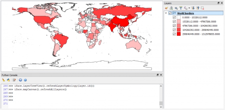
Lastly, here is an example that shows you how you can change the symbology of a layer from your code:
renderer = QgsGraduatedSymbolRenderer()
renderer.setClassAttribute('POP2005')
layer.setRenderer(renderer)
layer.renderer().updateClasses(layer, QgsGraduatedSymbolRenderer.Jenks, 5)
layer.renderer().updateColorRamp(QgsGradientColorRamp(Qt.white, Qt.red))
iface.layerTreeView().refreshLayerSymbology(layer.id())
iface.mapCanvas().refreshAllLayers()
Here we create an object of the QgsGraduatedSymbolRenderer class that we want to use to draw the country polygons from our layer using a graduated color approach based on the population attribute ‘POP2005’. The name of the field to use is set via the renderer’s setClassAttribute() method in line 2. Then we make the renderer object the renderer for our world borders layer in line 3. In the next two lines, we tell the renderer (now accessed via the layer method renderer()) to use a Jenks Natural Breaks classification with 5 classes and a gradient color ramp that interpolates between the colors white and red. Please note that the colors used as parameters here are predefined instances of the Qt5 class QColor. Changing the symbology does not automatically refresh the map canvas or layer list. Therefore, in the last two lines, we explicitly tell the running QGIS environment to refresh the symbology of the world borders layer in the Layers tree view (line 6) and to refresh the map canvas (line 7). The result should look similar to the figure below (with all other layers removed).
You will get to see another example of interacting with the layers open in QGIS and setting the symbology (for point and line layers in this case) in Section 4.12 where we take the code from this lesson's walkthrough and turn it into a QGIS plugin.
[1] The qgis Python module is a wrapper around the underlying C++ library. The documentation pages linked in this section are those of the C++ version but the names of classes and available functions and methods are the same.
4.5.2 Accessing the Features of a Layer
Let’s keep working with the world borders layer open in QGIS for a bit, looking at how we can access the individual features in a layer and select features by attribute. The following piece of code shows you how we can loop through all the features with the help of the layer’s getFeatures() method:
for feature in layer.getFeatures():
    print(feature)
    print(feature.id())
    print(feature['NAME'])
    print('-----')
Output:
<qgis._core.QgsFeature object at 0x...>
0
Antigua and Barbuda
-----
<qgis._core.QgsFeature object at 0x...>
1
Algeria
-----
<qgis._core.QgsFeature object at 0x...>
2
Azerbaijan
-----
<qgis._core.QgsFeature object at 0x...>
3
Albania
-----
...
Features are represented as objects of the class QgsFeature [24] in QGIS. So, for each iteration of the for-loop in the previous code example, variable feature will contain a QgsFeature object. Features are numbered with a unique ID that you can obtain by calling the method id() as we are doing in this example. Attributes like the NAME attribute of the world borders polygons can be accessed using the attribute name as the key as also demonstrated above.
Like in most GIS software, a layer can have an active selection. When the layer is open in QGIS, the selected features are highlighted. The layer method selectAll() allows for selecting all features in a layer and removeSelection() can be used to clear the selection. Give this a try by running the following two commands in the QGIS Python console and watch how all countries become selected and then deselected again.
layer.selectAll()
layer.removeSelection()
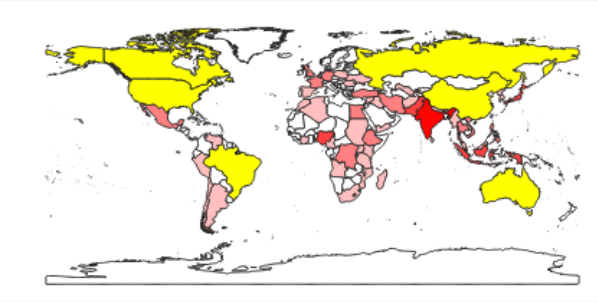
The method selectByExpression() allows for selecting features based on their properties with a SQL query string that has the same format as in ArcGIS. Use the following command to select all features from the layer that have a value larger than 300,000 in the AREA column of the attribute table. The result should look as in the figure below.
layer.selectByExpression('"AREA" > 300000')
While there can only be one active selection for a layer, you can create as many subgroups of features from a layer as you want by calling getFeatures(…) with a parameter that is an object of the class QgsFeatureRequest [25] and that has been given a filter expression via its setFilterExpression(…) method. The filter expression can be again an SQL query string. The following code creates a subgroup that will only contain the polygon for Canada. When you run it, this will not change the active selection that you see for that layer in QGIS but variable selectionName now provides access to the subgroup with just that one polygon. We get that first (and only) polygon by calling the __next__() method of selectionName and then print out some information about this particular polygon feature.
selectionName = layer.getFeatures(QgsFeatureRequest().setFilterExpression('"NAME" = \'Canada\''))
feature = selectionName.__next__()
print(feature['NAME'] + "-" + str(feature.id()))
print(feature.geometry())
print(feature.geometry().asWkt())
Output:
Canada – 23
<qgis._core.QgsGeometry object at 0x...>
MultiPolygon (((-65.61361699999997654 43.42027300000000878,...)))
The first print statement in this example works in the same way as you have seen before to get the name attribute and id of the feature. The method geometry() gives us the geometric object for this feature as an instance of the QgsGeometry class [26] and calling the method asWkt() gives us a WKT string representation of the multi-polygon geometry. You can also use a for-loop to iterate through the features in a subgroup created in this way. The method rewind() can be used to reset the iterator to the beginning so that when you call __next__() again, it will again give you the first feature from the subgroup.
When you have the geometry object and know what type of geometry it is, you can use the methods asPoint(), asPolygon(), asPolyline(), asMultiPolygon(), etc. to get the geometry as a Python data structure, e.g. in the case of multi-polygons as a list of lists of lists with each inner list containing tuples of the point coordinates for one polygonal component.
print(feature.geometry().asMultiPolygon())
[[[(-65.6136, 43.4203), (-65.6197,43.4181), … ]]]
Here is another example to demonstrate that we can work with several different subgroups of features at the same time. This time we request all features from the layer that have a POP2005 value larger than 50,000,000.
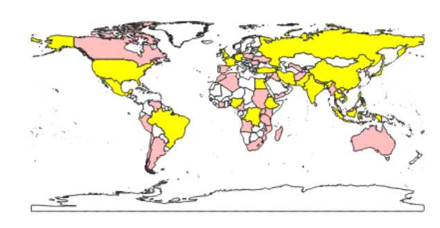
selectionPopulation = layer.getFeatures(QgsFeatureRequest().setFilterExpression('"POP2005" > 50000000'))
If we ever want to use a subgroup like this to create the active selection for the layer from it, we can use the layer method selectByIds(…) for this. The method requires a list of feature IDs and will then change the active selection to these features. In the following example, we use a simple list comprehension to create the ID list from the subgroup in our variable selectionPopulation:
layer.selectByIds([f.id() for f in selectionPopulation])
When running this command you should notice that the selection of the features in QGIS changes to look like in the figure below.
Let’s save the currently selected features as a new file. We use the GeoPackage format (GPKG) for this, which is more modern than the shapefile format, but you can easily change the command below to produce a shapefile instead; simply change the file extension to “.shp” and replace “GPKG” with “ESRI Shapefile”. The function we will use for writing the layer to disk is called writeAsVectorFormat(…) and it is defined in the class QgsVectorFileWriter [27]. Please note that this function has been declared "deprecated", meaning it may be removed in future versions and it is recommended that you do not use it anymore. In versions up to QGIS 3.16 (the current LTR version that most likely you are using right now), you are supposed to use writeAsVectorFormatV2(...) instead; however, there have been issues reported with that function and it is already replaced by writeAsVectorFormatV3(...) in versions >3.16 of QGIS. Therefore, we have decided to stick with writeAsVectorFormat(…) while things are still in flux. The parameters we give to writeAsVectorFormat(…) are the layer we want to save, the name of the output file, the character encoding to use, the spatial reference to use (we simply use the one that our layer is in), the format (“GPKG”), and True for signaling that only the selected features should be saved in the new data set. Adapt the path for the output file as you see fit and then run the command:
QgsVectorFileWriter.writeAsVectorFormat(layer, r'C:\489\highPopulationCountries.gpkg', 'utf-8', layer.crs(),'GPKG', True)
If you add the new file produced by this command to your QGIS project, it should only contain the polygons for the countries we selected based on their population values.
For changing the attribute values of a feature, we need to work with the “data provider” object of the layer. We can access it via the layer’s dataProvider() method:
dataProvider = layer.dataProvider()
Let’s say we want to change the POP2005 value for Canada to 1 (don’t ask what happened!). For this, we also need the index of the POP2005 column which we can get by calling the data provider’s fieldNameIndex() method:
populationColumnIndex = dataProvider.fieldNameIndex('POP2005')
To change the attribute value we call the method changeAttributeValues(…) of the data provider object providing a dictionary as parameter that maps feature IDs to dictionaries which in turn map column indices to new values. The inner dictionary that maps column indices to values is defined in a separate variable newValueDictionary.
newValueDictionary = { populationColumnIndex : 1 }
dataProvider.changeAttributeValues( { feature.id(): newValueDictionary } )
In this simple example, the outer dictionary contains only a single key-value pair with the ID of the feature for Canada as key and another dictionary as value. The inner dictionary also only contains a single key-value pair consisting of the index of the population column and its new value 1. Both dictionaries can have multiple entries to simultaneously change multiple values of multiple features. After running this command, check out the attributes of Canada, either via the QGIS Identify tool or in the attribute table of the layer. You will see that the population value in the layer now has been changed to 1 (the same holds for the underlying shapefile). Let’s set the value back to what it was with the following command:
dataProvider.changeAttributeValues( { feature.id(): { populationColumnIndex : 32270507 } } )
4.5.3 Creating Features and Geometric Operations
For the final part of this section, let’s switch from the Python console in QGIS to writing a standalone script that uses qgis. You can use your editor of choice to write the script and then execute the .py file from the OSGeo4W shell (see again Section 4.4.1) with all environment variables set correctly for a qgis and QT5 based program.
We are going to repeat the task from Section 3.9.1 of creating buffers around the centroids of the countries within a rectangular (in terms of WGS 84 coordinates) area around southern Africa. We will produce two new vector GeoPackage files: a point based one with the centroids and a polygon based one for the buffers. Both data sets will only contain the country name as their only attribute.
We start by importing the modules we will need and creating a QApplication() (handled by qgis.core.QgsApplication) for our program that qgis can run in (even though the program does not involve any GUI).
Important note: When you later write you own qgis programs (e.g. in the L4 homework assignment), make sure that you always "import qgis" first before using any other qgis related import statements such as "import qgis.core". We are not sure why this is needed, but the other imports will most likely fail tend to fail without "import qgis" coming first.
import os, sys
import qgis
import qgis.core
To use qgis in our software, we have to initialize it and we need to tell it where the actual QGIS installation is located. To do this, we use the function getenv(…) of the os module to get the value of the environmental variable “QGIS_PREFIX_PATH” which will be correctly defined when we run the program from the OSGeo4W shell. Then we create an instance of the QgsApplication class and call its initQgis() method.
qgis_prefix = os.getenv("QGIS_PREFIX_PATH")
qgis.core.QgsApplication.setPrefixPath(qgis_prefix, True)
qgs = qgis.core.QgsApplication([], False)
qgs.initQgis()
Now we can implement the main functionality of our program. First, we load the world borders shapefile into a layer (you may have to adapt the path!).
layer = qgis.core.QgsVectorLayer(r'C:\489\TM_WORLD_BORDERS-0.3.shp')
Then we create the two new layers for the centroids and buffers. These layers will be created as new in-memory layers and later written to GeoPackage files. We provide three parameters to QgsVectorLayer(…): (1) a string that specifies the geometry type, coordinate system, and fields for the new layer; (2) a name for the layer; and (3) the string “memory” which tells the function that it should create a new layer in memory from scratch (rather than reading a data set from somewhere else as we did earlier).
centroidLayer = qgis.core.QgsVectorLayer("Point?crs=" + layer.crs().authid() + "&field=NAME:string(255)", "temporary_points", "memory")
bufferLayer = qgis.core.QgsVectorLayer("Polygon?crs=" + layer.crs().authid() + "&field=NAME:string(255)", "temporary_buffers", "memory")
The strings produced for the first parameters will look like this: “Point?crs=EPSG:4326&field=NAME:string(255)” and “Polygon?crs=EPSG:4326&field=NAME:string(255)”. Note how we are getting the EPSG string from the world border layer so that the new layers use the same coordinate system, and how an attribute field is described using the syntax “field=<name of the field>:<type of the field>". When you want your layer to have more fields, these have to be separated by additional & symbols like in a URL.
Next, we set up variables for the data providers of both layers that we will need to create new features for them. The new features will be collected in two lists, centroidFeatures and bufferFeatures.
centroidProvider = centroidLayer.dataProvider()
bufferProvider = bufferLayer.dataProvider()

centroidFeatures = []
bufferFeatures = []
Then, we create the polygon geometry for our selection area from a WKT string as in Section 3.9.1:
areaPolygon = qgis.core.QgsGeometry.fromWkt('POLYGON ( (6.3 -14, 52 -14, 52 -40, 6.3 -40, 6.3 -14) )')
In the main loop of our program, we go through all the features in the world borders layer, use the geometry method intersects(…) to test whether the country polygon intersects with the area polygon, and, if yes, create the centroid and buffer features for the two layers from the input feature.
for feature in layer.getFeatures():
    if feature.geometry().intersects(areaPolygon):
        centroid = qgis.core.QgsFeature()
        centroid.setAttributes([feature['NAME']])
        centroid.setGeometry(feature.geometry().centroid())
        centroidFeatures.append(centroid)

        buffer = qgis.core.QgsFeature()
        buffer.setAttributes([feature['NAME']])
        buffer.setGeometry(feature.geometry().centroid().buffer(2.0,100))
        bufferFeatures.append(buffer)
Note how in both cases (centroids and buffers), we first create a new QgsFeature object, then use setAttributes(…) to set the NAME attribute to the name of the country, and then use setGeometry(…) to set the geometry of the new feature either to the centroid derived by calling the centroid() method or to the buffered centroid created by calling the buffer(…) method of the centroid point. As a last step, the new features are added to the respective lists. Finally, all features in the two lists are added to the layers after the for-loop has been completed. This happens with the following two commands:
centroidProvider.addFeatures(centroidFeatures)
bufferProvider.addFeatures(bufferFeatures)
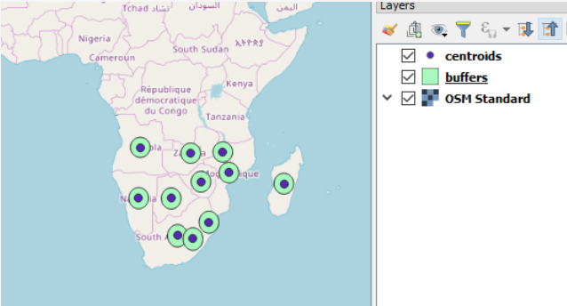
Lastly, we write the content of the two in-memory layers to GeoPackage files on disk. This works in the same way as in previous examples. Again, you might want to adapt the output paths.
qgis.core.QgsVectorFileWriter.writeAsVectorFormat(centroidLayer, r'C:\489\centroids.gpkg', "utf-8", layer.crs(), "GPKG")
qgis.core.QgsVectorFileWriter.writeAsVectorFormat(bufferLayer, r'C:\489\buffers.gpkg', "utf-8", layer.crs(), "GPKG")
Since we are now done with using QGIS functionalities (and actually the entire program), we clean up by calling the exitQgis() method of the QgsApplication, freeing up resources that we don’t need anymore.
qgs.exitQgis()
If you run the program from the OSGeo4W shell and then open the two produced output files in QGIS, the result should look as shown in the image below.
4.5.4 (Geo)processing
QGIS has a toolbox system and visual workflow building component somewhat similar to ArcGIS and its Model Builder. It is called the QGIS processing framework [28]and comes in the form of a plugin called Processing that is installed by default. You can access it via the Processing menu in the main menu bar. All algorithms from the processing framework are available in Python via a QGIS module called processing. They can be combined to solve larger analysis tasks in Python and can also be used in combination with the other qgis methods discussed in the previous sections.
We can get a list of all processing algorithms currently registered with QGIS with the command QgsApplication.processingRegistry().algorithms(). Each processing object in the returned list has an identifying name that you can get via its id() method. The following command, which you can try out in the QGIS Python console, uses this approach to print the names of all algorithms that contain the word “clip”:
[x.id() for x in QgsApplication.processingRegistry().algorithms() if "clip" in x.id()]
Output:

['gdal:cliprasterbyextent', 'gdal:cliprasterbymasklayer','gdal:clipvectorbyextent', 'gdal:clipvectorbypolygon', 'native:clip', 'saga:clippointswithpolygons', 'saga:cliprasterwithpolygon', 'saga:polygonclipping']
As you can see, there are processing versions of algorithms coming from different sources, e.g. natively built into QGIS vs. algorithms based on GDAL. The function algorithmHelp(…) allows you to get some documentation on an algorithm and its parameters. Try it out with the following command:
processing.algorithmHelp("native:clip")
To run a processing algorithm, you have to use the run(…) function and provide two parameters: the id of the algorithm and a dictionary that contains the parameters for the algorithm as key-value pairs. run(…) returns a dictionary with all output parameters of the algorithm. The following example illustrates how processing algorithms can be used to solve the task of clipping a points of interest shapefile to the area of El Salvador, reusing the two data sets from homework assignment 2 (Section 2.10). This example is intended to be run as a standalone program again and most of the code is required to set up the QGIS environment needed, including initializing the Processing environment.
The start of the script looks like in the example from the previous section:
import os,sys
import qgis
import qgis.core

qgis_prefix = os.getenv("QGIS_PREFIX_PATH")
qgis.core.QgsApplication.setPrefixPath(qgis_prefix, True)
qgs = qgis.core.QgsApplication([], False)
qgs.initQgis()
After, creating the QGIS environment, we can now initialize the processing framework. To be able to import the processing module we have to make sure that the plugins folder is part of the system path; we do this directly from our code. After importing processing, we have to initialize the Processing environment and we also add the native QGIS algorithms to the processing algorithm registry.
# Be sure to change the path to point to where your plugins folder is located
# it may not be the same as this one.
sys.path.append(r"C:\OSGeo4W\apps\qgis-ltr\python\plugins")
import processing
from processing.core.Processing import Processing
Processing.initialize()
qgis.core.QgsApplication.processingRegistry().addProvider(qgis.analysis.QgsNativeAlgorithms())
Next, we create input variables for all files involved, including the output files we will produce, one with the selected country and one with only the POIs in that country. We also set up input variables for the name of the country and the field that contains the country names.
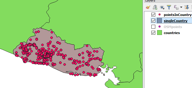
poiFile = r'C:\489\L2\assignment\OSMpoints.shp'
countryFile = r'C:\489\L2\assignment\countries.shp'
pointOutputFile = r'C:\489\L2\assignment\pointsInCountry.shp'
countryOutputFile = r'C:\489\L2\assignment\singleCountry.shp'

nameField = "NAME"
countryName = "El Salvador"
Now comes the part in which we actually run algorithms from the processing framework. First, we use the qgis:extractbyattribute algorithm to create a new shapefile with only those features from the country data set that satisfy a particular attribute query. In the dictionary with the input parameters for the algorithm, we specify the name of the input file (“INPUT”), the name of the query field (“FIELD”), the comparison operator for the query (0 here stands for “equal”), and the value to which we are comparing (“VALUE”). Since the output will be written to a new shapefile, we don’t really need the output dictionary that we get back from calling run(…) but the print statement shows how this dictionary in this case contains the name of the output file under the key “OUTPUT”.
output = processing.run("qgis:extractbyattribute", { "INPUT": countryFile, "FIELD": nameField, "OPERATOR": 0, "VALUE": countryName, "OUTPUT": countryOutputFile  })
print(output['OUTPUT'])
To perform the clip operation with the new shapefile from the previous step, we use the “native:clip” algorithm. The input paramters are the input file (“INPUT”), the clip file (“OVERLAY”), and the output file (“OUTPUT”). Again, we are just printing out the content stored under the “OUTPUT” key in the returned dictionary. Finally, we exit the QGIS environment.
output = processing.run("native:clip", { "INPUT": poiFile, "OVERLAY": countryOutputFile, "OUTPUT": pointOutputFile })
print(output['OUTPUT'])

qgs.exitQgis()
Below is how the resulting two layers should look when shown in QGIS in combination with the original country layer.
In this section, we showed you how to perform common GIS operations with the QGIS Python API. Once again we have to say that we are only scratching the surface here; the API is much more complex and powerful, and there is hardly anything you cannot do with it. What we have shown you will be sufficient to understand the code from the two walkthroughs of this lesson, but, if you want more, below are some links to further examples. Keep in mind though that since QGIS 3 is not that old yet, some of the examples on the web have been written for QGIS 2.x. While many things still work in the same way in QGIS 3, you may run into situations in which an example won’t work and needs to be adapted to be compatible with QGIS 3.
4.6 Object-Oriented Programming in Python
GEOG 485 already described some of the fundamental ideas of object-oriented programming and you have been using objects of classes defined in different Python packages like arcpy quite a bit. For instance, you have been creating new objects of the arcpy Point or Array classes by writing something like
p = arcpy.Point()
points = arcpy.Array()
You have also been accessing properties of the objects created, e.g. by writing
p.X
... to get the x coordinate of the Point object stored in variable p. And you have been invoking methods of objects, for instance the add(…) method to add a point to the Array stored in variable points:
points.add(p)
What we did not cover in GEOG485 is how to define your own classes in Python, derive new classes from already existing ones to create class hierarchies, and use these ideas to build larger software applications with a high degree of readability, maintainability, and reusability. All these things will be covered in this and the next section and put into practice throughout the rest of this lesson.
4.6.1 Classes, Objects, and Methods
Let’s recapitulate a bit: the underlying perspective of object-oriented programming is that the domain modeled in a program consists of objects belonging to different classes. If your software models some part of the real world, you may have classes for things like buildings, vehicles, trees, etc. and then the objects (also called instances) created from these classes during run-time represent concrete individual buildings, vehicles, or trees with their specific properties. The classes in your software can also describe non real-world and often very abstract things like a feature layer or a random number generator.
Class definitions specify general properties that all objects of that class have in common, together with the things that one can do with these objects. Therefore, they can be considered blueprints for the objects. Each object at any moment during run-time is in a particular state that consists of the concrete values it has for the properties defined in its class. So, for instance, the definition of a very basic class Car may specify that all cars have the properties owner, color, currentSpeed, and lightsOn. During run-time we might then create an object for “Tom’s car” in variable carOfTom with the following values making up its state:
carOfTom.owner = "Tom"
carOfTom.color = "blue"
carOfTom.currentSpeed = 48   (mph)
carOfTom.lightsOn = False
While all objects of the same class have the same properties (also called attributes or fields), their values for these properties may vary and, hence, they can be in different states. The actions that one can perform with a car or things that can happen to a car are described in the form of methods in the class definition. For instance, the class Car may specify that the current speed of cars can be changed to a new value and that lights can be turned on and off. The respective methods may be called changeCurrentSpeed(…), turnLightsOn(), and turnLightsOff(). Methods are like functions but they are explicitly invoked on an object of the class they are defined in. In Python this is done by using the name of the variable that contains the object, followed by a dot, followed by the method name:
carOfTom.changeCurrentSpeed(34) # change state of Tom’s car to current speed being 34mph

carOfTom.turnLightsOn()         # change state of Tom’s car to lights being turned on
The purpose of methods can be to update the state of the object by changing one or several of its properties as in the previous two examples. It can also be to get information about the state of the car, e.g. are the lights turned on? But it can also be something more complicated, e.g. performing a certain driving maneuver or fuel calculation.
In object-oriented programming, a program is perceived as a collection of objects that interact by calling each other’s methods. Object-oriented programming adheres to three main design principles:
- Encapsulation: Definitions related to the properties and methods of any class appear in a specification that is encapsulated independently from the rest of the software code and properties are only accessible via a well-defined interface, e.g. via the defined methods.
- Inheritance: Classes can be organized hierarchically with new classes being derived from previously defined classes inheriting all the characteristics of the parent class but potentially adding specialized properties or specialized behavior. For instance, our class Car could be derived from a more general class Vehicle adding properties and methods that are specific for cars.
- Polymorphism: Inherited classes can change the behavior of methods by overwriting them and the code executed when such a method is invoked for an object then depends on the class of that object.
We will talk more about inheritance and polymorphism in section 4.8. All three principles aim at improving reusability and maintainability of software code. These days, most software is created by mainly combining parts that already exist because that saves time and costs and increases reliability when the re-used components have already been thoroughly tested. The idea of classes as encapsulated units within a program increases reusability because these units are then not dependent on other code and can be moved over to a different project much more easily.
For now, let’s look at how our simple class Car can be defined in Python.
 class Car():

     def __init__(self):
          self.owner = 'UNKNOWN'
          self.color = 'UNKNOWN'
          self.currentSpeed = 0
          self.lightsOn = False

     def changeCurrentSpeed(self,newSpeed):
          self.currentSpeed = newSpeed

     def turnLightsOn(self):
          self.lightsOn = True

     def turnLightsOff(self):
          self.lightsOn = False

     def printInfo(self):
          print('Car with owner = {0}, color = {1}, currentSpeed = {2}, lightsOn = {3}'.format(self.owner, self.color, self.currentSpeed, self.lightsOn))
Here is an explanation of the different parts of this class definition: each class definition in Python starts with the keyword ‘class’ followed by the name of the class (‘Car’) followed by parentheses that may contain names of classes that this class inherits from, but that’s something we will only see later on. The rest of the class definition is indented to the right relative to this line.
The rest of the class definition consists of definitions of the methods of the class which all look like function definitions but have the keyword ‘self’ as the first parameter, which is an indication that this is a method. The method __init__(…) is a special method called the constructor of the class. It will be called when we create a new object of that class like this:
carOfTom = Car() # uses the __init__() method of Car to create a new Car object
In the body of the constructor, we create the properties of the class Car. Each line starting with “self.<name of property> = ...“ creates a so-called instance variable for this car object and assigns it an initial value, e.g. zero for the speed. The instance variables describing the state of an object are another type of variable in addition to global and local variables that you already know. They are part of the object and exist as long as that object exists. They can be accessed from within the class definition as “self.<name of the instance variable>” which happens later in the definitions of the other methods, namely in lines 10, 13, 16 and 19. If you want to access an instance variable from outside the class definition, you have to use <name of variable containing the object>.<name of the instance variable>, so, for instance:
print(carOfTom.lightsOn) # will produce the output False because right now this instance variable still has its default value
The rest of the class definition consists of the methods for performing certain actions with a Car object. You can see that the already mentioned methods for changing the state of the Car object are very simple. They just assign a new value to the respective instance variable, a new speed value that is provided as a parameter in the case of changeCurrentSpeed(…) and a fixed Boolean value in the cases of turnLightsOn() and turnLightsOff(). In addition, we added a method printInfo() that prints out a string with the values of all instance variables to provide us with all information about a car’s current state. Let us now create a new instance of our Car class and then use some of its methods:
carOfSue = Car()
carOfSue.owner = 'Sue'
carOfSue.color = 'white'
carOfSue.changeCurrentSpeed(41)
carOfSue.turnLightsOn()
carOfSue.printInfo()
Output:

Car with owner = Sue, color = white, currentSpeed = 41, lightsOn = True
Since we did not define any methods to change the owner or color of the car, we are directly accessing these instance variables and assigning new values to them in lines 2 and 3. While this is okay in simple examples like this, it is recommended that you provide so-called getter and setter methods (also called accessor and mutator methods) for all instance variables that you want the user of the class to be able to read (“get”) or change (“set”). The methods allow the class to perform certain checks to make sure that the object always remains in an allowed state. How about you go ahead and for practice create a second car object for your own car (or any car you can think of) in a new variable and then print out its information?
A method can call any other method defined in the same class by using the notation “self.<name of the method>(...)”. For example, we can add the following method randomSpeed() to the definition of class Car:
def setRandomSpeed(self):
    self.changeCurrentSpeed(random.randint(0,76))
The new method requires the “random” module to be imported at the beginning of the script. The method generates a random number and then uses the previously defined method changeCurrentSpeed(…) to actually change the corresponding instance variable. In this simple example, one could have simply changed the instance variable directly but in more complex cases changes to the state can require more code so that this approach here actually avoids having to repeat that code. Give it a try and add some lines to call this new method for one of the car objects and then print out the info again.
4.6.2 Constructors with parameters and defining the == and < operators
It can be a bit cumbersome to use methods or assignments to set all the instance variables to the desired initial values after a new object has been created. Instead, one would rather like to pass initial values to the constructor and get back an object with these values for the instance variables. It is possible to do so in Python by adding additional parameters to the constructor. Go ahead and change the definition of the constructor in class Car to the following version:
def __init__(self, owner = 'UNKNOWN', color = 'UNKNOWN', currentSpeed = 0, lightsOn = False):
	self.owner = owner
	self.color = color
	self.currentSpeed = currentSpeed
	self.lightsOn = lightsOn
Please note that we here used identical names for the instance variables and corresponding parameters of the constructor used for providing the initial values. However, these are still distinguishable because instance variables always have the prefix “self.”. In this new version of the constructor we are using keyword arguments for each of the properties to provide maximal flexibility to the user of the class. The user can now use any combination of providing their own initial values or using the default values for these properties. Here is how to re-create Sue’s car by providing values for all the properties:
carOfSue = Car(owner='Sue', color='white', currentSpeed = 41, lightsOn = True)
carOfSue.printInfo()
Output:

Car with owner = Sue, color = white, currentSpeed = 41, lightsOn = True
Here is a version in which we only specify the owner and the speed. Surely you can guess what the output will look like.
carOfSue = Car(owner='Sue', currentSpeed = 41)
carOfSue.printInfo()
In addition to __init__(…) for the constructor, there is another special method called __str__(). This method is called by Python when you either explicitly convert an object from that class to a string using the Python str(…) function or implicitly, e.g. when printing out the object with print(…). Try out the following two commands for Sue’s car and see what output you get:
print(str(carOfSue))
print(carOfSue)
Now add the following method to the definition of class Car:
	def __str__(self):
            return 'Car with owner = {0}, color = {1}, currentSpeed = {2}, lightsOn = {3}'.format(self.owner, self.color, self.currentSpeed, self.lightsOn)
Now repeat the two commands from above and look at the difference. The output should now be the following line repeated twice:
Car with owner = Sue, color = UNKNOWN, currentSpeed = 41, lightsOn = False
For implementing the method, we simply used the same string that we were printing out from the printInfo() method. In principal, this method is not really needed anymore now and could be removed from the class definition.
Objects can be used like any other value in Python code. Actually, everything in Python is an object, even primitive data types like numbers and Boolean values. That means we can …
- use objects as parameters of functions and methods (you will see an example of this with the function stopCar(…) defined below),
- return objects as the return value of a function or method,
- store objects inside sequences or containers, for instance in lists like this: carList = [ carOfTom, carOfSue, Car(owner = 'Mike'],
- store objects in instance variables of other objects.
To illustrate this last point, we can add another class to our car example, one for representing car manufacturers:
class Manufacturer():
     def __init__(self, name):
          self.name = name
Usually such a class would be much more complex, containing additional properties for describing a concrete car manufacturer. But we keep things very simple here and say that the only property is the name of the manufacturer. We now modify the beginning of the definition of class Car so that another instance variable is created called self.manufacturer. This is used for storing an object of class Manufacturer inside each Car object for representing the manufacturer of that particular car. For parameters that are objects of classes, it is common to use the special value None as the default value when the parameter is not provided.
class Car():

     def __init__(self, manufacturer = None, owner = 'UNKNOWN', color = 'UNKNOWN', currentSpeed = 0, lightsOn = False):
        self.manufacturer = manufacturer
        self.owner = owner
        self.color =  color
        self.currentSpeed = currentSpeed
        self.lightsOn = lightsOn
The rest of the class definition can stay the same although we would typically change the __str__(...) method to include this new instance variable. The following code shows how to create a new Car object by first creating a Manufacturer object with name 'Chrysler'. This object could also come from a predefined list or dictionary of car manufacturer objects if we want to be able to use the same Manufacturer object for several cars. Then we use this object for the manufacturer keyword argument of the Car constructor. As a result, this object gets assigned to the manufacturer instance variable of the car as reflected by the output from the final print statement.
m = Manufacturer('Chrysler')
carOfFrank = Car(manufacturer = m, owner = 'Frank', currentSpeed = 70)
print(carOfFrank.manufacturer.name)
Output:
Chrysler
Note how in the last line of the example above, we chain things together via dots starting from the variable containing the car object (carOfFrank), followed by the name of an instance variable (manufacturer) of class Car, followed by the name of an instance variable of class Manufacturer (name): carOfFrank.manufacturer.name . This is also something you have probably seen before, for instance as “describeObject.SpatialReference.Name” when accessing the name of the spatial reference object that is stored inside an arcpy Describe object.
We briefly discussed in Section 4.2 when talking about collections that when defining our own classes we may have to provide definitions of comparison operators like == and < for them to work as we wish when placed into a collection. So a question for instance would be, when should two car objects be considered to be equal? We could take the standpoint that they are equal if the values of all instance variables are equal. Or it could make sense for a particular application to define that two Car objects are equal if the name of the owner and the manufacturer are equal. If our instance variables would include the license plate number that would obviously make for a much better criterion. Similarly, let us say we want to keep our Car objects in a priority queue sorted by their current speed values. In that case, we need to define the < comparison operator so that car A < car B holds if the value of the currentSpeed variable of A is smaller than that of B.
The meaning of the == operator is defined via a special method called __eq__(…) for “equal”, while that of the < operator is defined in a special method called __lt__(…) for “less than”. The following code example extends the most recent version of our class Car with a definition of the __eq__(…) method based on the idea that cars should be treated as equal if owner and manufacturer are equal. It then uses a Python list with a single car object and another car object with the same owner and manufacturer but different speed to illustrate that the new definition works as intended for the list operations “in” and index(…).
class Car():

    … # just add the method below to the previous definition of the class

    def __eq__(self, otherCar):
        return self.owner == otherCar.owner and self.manufacturer == otherCar.manufacturer

m = 'Chrysler'
carList = [ Car(owner='Sue', currentSpeed = 41, manufacturer = m) ]
car = Car(owner='Sue', currentSpeed = 0, manufacturer = m)

if car in carList:
    print('Already contained in the list')
print(carList.index(car))
Output:
Already contained in the list
0
Note that __eq__(…) takes another Car object as parameter and then simply compares the values of the owner and manufacturer instance variables of the Car object the method was called for with the corresponding values of that other Car object. The output shows that Python considers the car to be already located in the list as the first element, even though these are actually two different car objects with different speed values. This is because these operations use the new definition of the == operator for objects of our class Car that we provided with the method __eq__(...).
You now know the basics of writing own classes in Python and how to instantiate them and use the created objects. To wrap up this section, let’s come back to a topic that we already discussed in Section 1.4 of Lesson 1. Do you remember the difference between mutable and immutable objects when given as a parameter to functions? Mutable objects like lists used as parameters can be changed within the function. All objects that we create from classes are also mutable, so you can in principle write code like this:
def stopCar(car):
	car.currentSpeed = 0

stopCar(carOfFrank)
print(carOfFrank)
When stopCar(...) is called, the parameter car will refer to the same car object that variable carOfFrank is referring to. Therefore, all changes made to that object inside the function referring to variable car will be reflected by the final print statement for carOfFrank showing a speed of 0. What we have not discussed so far is that there is a second situation where this is important, namely when making an assignment. You may think that when you write something like
anotherCar = carOfFrank
a new variable will be created and a copy of the car object in variable carOfFrank will be assigned to that variable so that you can make changes to the instance variables of that object without changing the object in carOfFrank. However, that is only how it works for immutable values. Instead, after the assignment, both variables will refer to the same Car object in memory. Therefore, when you add the following commands
anotherCar.color = 'green'
anotherCar.changeCurrentSpeed(12)
print(carOfFrank)
The output will be:
Car with owner = Frank, color = green, currentSpeed = 12, lightsOn = False
It works in the same way for all mutable objects, so also for lists for example. If you want to create an independent copy of a mutable object, the module copy [32] from the Python standard library contains the functions copy(…) and deepcopy(…) to explicitly create copies. The difference between the two functions is explained in the documentation and only plays a role when the object to be copied contains other objects, e.g. if you want to make a copy of a list of Car objects.
4.7 Inheritance, Class Hierarchies and Polymorphism
We already mentioned building class hierarchies via inheritance and polymorphism as two main principles of object-oriented programming in addition to encapsulation. To introduce you to these concepts, let us start with another exercise in object-oriented modeling and writing classes in Python. Imagine that you are supposed to write a very basic GIS or vector drawing program that only deals with geometric features of three types: circles, and axis-aligned rectangles and squares. You need the ability to store and manage an arbitrary number of objects of these three kinds and be able to perform simple operations with these objects like computing their area and perimeter and moving the objects to a different position. How would you write the classes for these three kinds of geometric objects?
Let us start with the class Circle: a circle in a two-dimensional coordinate system is typically defined by three values, the x and y coordinates of the center of the circle and its radius. So these should become the properties (= instance variables) of our Circle class and for computing the area and perimeter, we will provide two methods that return the respective values. The method for moving the circle will take the values by how much the circle should be moved along the x and y axes as parameters but not return anything.
import math

class Circle():
	def __init__(self, x = 0.0, y = 0.0, radius = 1.0):
		self.x = x
		self.y = y
		self.radius = radius

    def computeArea(self):
	    return math.pi * self.radius ** 2

    def computePerimeter (self):
	    return 2 * math.pi * self.radius

    def move(self, deltaX, deltaY):
	    self.x += deltaX
	    self.y += deltaY

    def __str__(self):
	    return 'Circle with coordinates {0}, {1} and radius {2}'.format(self.x, self.y, self.radius)
In the constructor, we have keyword arguments with default values for the three properties of a circle and we assign the values provided via these three parameters to the corresponding instance variables of our class. We import the math module of the Python standard library so that we can use the constant math.pi for the computations of the area and perimeter of a circle object based on the instance variables. Finally, we add the __str__() method to produce a string that describes a circle object with its properties. It should by now be clear how to create objects of this class and, for instance, apply the computeArea() and move(…) methods.
circle1 = Circle(10,4,3)
print(circle1)
print(circle1.computeArea())
circle1.move(3,-1)
print(circle1)
Output:
Circle with coordinates 10, 4 and radius 3
28.274333882308138
Circle with coordinates 13, 3 and radius 3
How about a similar class for axis-aligned rectangles? Such rectangles can be described by the x and y coordinates of one of their corners together with width and height values, so four instance variables taking numeric values in total. Here is the resulting class and a brief example of how to use it:
class Rectangle():
	def __init__(self, x = 0.0, y = 0.0, width = 1.0, height = 1.0):
		self.x = x
		self.y = y
		self.width = width
		self.height = height

    def computeArea(self):
		return self.width * self.height

    def computePerimeter (self):
		return 2 * (self.width + self.height)

    def move(self, deltaX, deltaY):
		self.x += deltaX
		self.y += deltaY

	def __str__(self):
		return 'Rectangle with coordinates {0}, {1}, width {2} and height {3}'.format(self.x, self.y, self.width, self.height )

rectangle1 = Rectangle(10,10,3,2)
print(rectangle1)
print(rectangle1.computeArea())
rectangle1.move(2,2)
print(rectangle1)
Output:
Rectangle with coordinates 10, 10, width 3 and height 2
6
Rectangle with coordinates 12, 12, width 3 and height 2
There are a few things that can be observed when comparing the two classes Circle and Rectangle we just created: the constructors obviously vary because circles and rectangles need different properties to describe them and, as a result, the calls when creating new objects for the two classes also look different. All the other methods have exactly the same signature, meaning the same parameters and the same kind of return value; just the way they are implemented differs. That means the different calls for performing certain actions with the objects (computing the area, moving the object, printing information about the object) also look exactly the same; it doesn’t matter whether the variable contains an object of class Circle or of class Rectangle. If you compare the two versions of the move(…) method, you will see that these even do not differ in their implementation, they are exactly the same!
This all is a clear indication that we are dealing with two classes of objects that could be seen as different specializations of a more general class for geometric objects. Wouldn’t it be great if we could now write the rest of our toy GIS program managing a set of geometric objects without caring whether an object is a Circle or a Rectangle in the rest of our code? And, moreover, be able to easily add classes for other geometric primitives without making any changes to all the other code, and in their class definitions only describe the things in which they differ from the already defined geometry classes? This is indeed possible by arranging our geometry classes in a class hierarchy starting with an abstract class for geometric objects at the top and deriving child classes for Circle and Rectangle from this class with both adding their specialized properties and behavior. Let’s call the top-level class Geometry. The resulting very simple class hierarchy is shown in the figure below.
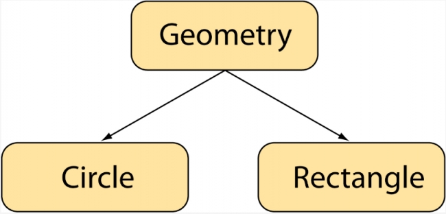
Inheritance allows the programmer to define a class with general properties and behavior and derive one or more specialized subclasses from it that inherit these properties and behavior but also can modify them to add more specialized properties and realize more specialized behavior. We use the terms derived class and base class to refer to the two classes involved when one class is derived from another.
4.7.1 Implementing the class hierarchy
Let’s change our example so that both Circle and Rectangle are derived from such a general class called Geometry. This class will be an abstract class in the sense that it is not intended to be used for creating objects from. Its purpose is to introduce properties and templates for methods that all geometric classes in our project have in common.
class Geometry():

	def __init__(self, x = 0.0, y = 0.0):
		self.x = x
		self.y = y

	def computeArea(self):
    	pass

    def computePerimeter(self):
		pass

    def move(self, deltaX, deltaY):
		self.x += deltaX
		self.y += deltaY

    def __str__(self):
		return 'Abstract class Geometry should not be instantiated and derived classes should override this method!'
The constructor of class Geometry looks pretty normal, it just initializes the instance variables that all our geometry objects have in common, namely x and y coordinates to describe their location in our 2D coordinate system. This is followed by the definitions of the methods computeArea(), computePerimeter(), move(…), and __str__() that all geometry objects should support. For move(…), we can already provide an implementation because it is entirely based on the x and y instance variables and works in the same way for all geometry objects. That means the derived classes for Circle and Rectangle will not need to provide their own implementation. In contrast, you cannot compute an area or perimeter in a meaningful way just from the position of the object. Therefore, we used the keyword pass to indicate that we are leaving the body of the computeArea() and computePerimeter() methods intentionally empty. These methods will have to be overridden in the definitions of the derived classes with implementations of their specialized behavior. We could have done the same for __str__() but instead we return a warning message that this class should not have been instantiated.
It is worth mentioning that, in many object-oriented programming languages, the concepts of an abstract class (= a class that cannot be instantiated) and an abstract method (= a method that must be overridden in every subclass that can be instantiated) are built into the language. That means there exist special keywords to declare a class or method to be abstract and then it is impossible to create an object of that class or a subclass of it that does not provide an implementation for the abstract methods. In Python, this has been added on top of the language via a module in the standard library called abc [33] (for abstract base classes). Although we won’t be using it in this course, it is a good idea to check it out and use it if you get involved in larger Python projects. This Abstract Classes page [34] is a good source for learning more.
Here is our new definition for class Circle that is now derived from class Geometry. We also use a few commands at the end to create and use a new Circle object of this class to make sure everything is indeed working as before:
import math

class Circle(Geometry):

	def __init__(self, x = 0.0, y = 0.0, radius = 1.0):
		super(Circle,self).__init__(x,y)
		self.radius = radius

	def computeArea(self):
		return math.pi * self.radius ** 2

	def computePerimeter (self):
		return 2 * math.pi * self.radius

	def __str__(self):
		return 'Circle with coordinates {0}, {1} and radius {2}'.format(self.x, self.y, self.radius)

circle1 = Circle(10, 10, 10)
print(circle1.computeArea())
print(circle1.computePerimeter())
circle1.move(2,2)
print(circle1)
Here are the things we needed to do in the code:
- In line 3, we had to change the header of the class definition to include the name of the base class we are deriving Circle from (‘Geometry’) within the parentheses.
- The constructor of Circle takes the same three parameters as before. However, it only initializes the new instance variable radius in line 7. For initializing the other two variables it calls the constructor of its base class, so the class Geometry, in line 6 with the command “super(Circle,self).__init__(x,y)”. This is saying “call the constructor of the base class of class Circle and pass the values of x and y as parameters to it”. It is typically a good idea to call the constructor of the base class as the first command in the constructor of the derived class so that all general initializations are taken care off.
- Then we provide definitions of computeArea() and computePerimeter() that are specific for circles. These definitions override the “empty” definitions of the Geometry base class. This means whenever we invoke computeArea() or computePerimeter() for an object of class Circle, the code from these specialized definitions will be executed.
- Note that we do not provide any definition for method move(…) in this class definition. That means when move(…) will be invoked for a Circle object, the code from the corresponding definition in its base class Geometry will be executed.
- We do override the __str__() method to produce the same kind of string with information about all instance variables that we had in the previous definition. Note that this function accesses both the instance variables defined in the parent class Geometry as well as the additional one added in the definition of Circle.
The new definition of class Rectangle, now derived from Geometry, looks very much the same as that of Circle if you replace “Circle” with “Rectangle”. Only the implementations of the overridden methods look different, using the versions specific for rectangles.
class Rectangle(Geometry):

	def __init__(self, x = 0.0, y = 0.0, width = 1.0, height = 1.0):
		super(Rectangle, self).__init__(x,y)
		self.width = width
        self.height = height

	def computeArea(self):
		return self.width * self.height

	def computePerimeter (self):
		return 2 * (self.width + self.height)

	def __str__(self):
		return 'Rectangle with coordinates {0}, {1}, width {2} and height {3}'.format(self.x, self.y, self.width, self.height )

rectangle1 = Rectangle(15,20,4,5)
print(rectangle1.computeArea())
print(rectangle1.computePerimeter())
rectangle1.move(2,2)
print(rectangle1)
4.7.2 Adding another class to the hierarchy
Overall, the new definitions of Circle and Rectangle have gotten shorter and redundant code like the implementation of move(…) only appears once, namely in the most general class Geometry. Let’s add another class to the hierarchy, a class for axis-aligned Square objects. Of course, you could argue that our class Rectangle is already sufficient to represent such squares. That is correct but we want to illustrate how it would look if you specialize a class already derived from Geometry further and one could well imagine a more complex version of our toy GIS example in which squares would add some other form of specialization. The resulting class hierarchy will then look like in the image below. The new class Square is a derived class of class Rectangle (so Rectangle is its base class) but it is also indirectly derived from class Geometry. Therefore, we say both Geometry and Rectangle are superclasses of Square and Square is a subclass of both these classes. Please note that the way we have been introducing these terms here, the terms base and derived class desribe the relationship between two nodes directly connected by a single arrow in the hierarchy graph, while superclass and subclass are more general and describe the relationship between two classes that are connected via any number of directed arrows in the graph.
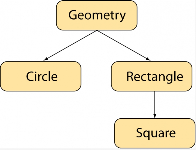
Here is the code for class Square:
class Square(Rectangle):

	def __init__(self, x = 0.0, y = 0.0, sideLength = 1.0):
		super(Square,self).__init__(x, y, sideLength, sideLength)

	def __str__(self):
		return 'Square with coordinates {0}, {1} and sideLength {2}'.format(self.x, self.y, self.width )

square1 = Square(5, 5, 8)
print(square1.computeArea())
print(square1.computePerimeter())
square1.move(2,2)
print(square1)
Right, the definition of Square is really short; we only define a new constructor that only takes x and y coordinates and a single sideLength value rather than width and height values. In the constructor we call the constructor of the base class Rectangle and provide sideLength for both the width and height parameters of that constructor. There are no new instance variables to initialize, so this is all that needs to happen in the constructor. Then the only other thing we have to do is override the __str__() method to produce some square-specific output message using self.width for the side length information for the square. (Of course, we could have just as well used self.height here.) The implementations of methods computeArea() and computePerimeter() are inherited from class Rectangle and the implementation of move(…) indirectly from class Geometry.
Now that we have this class hierarchy consisting of one abstract and three instantiable classes, the following code example illustrates the power of polymorphism. Imagine that in our toy GIS we have created a layer consisting of objects of the different geometry types. If we now want to implement a function computeTotalArea(…) that computes the combined area of all the objects in a layer, this can be done like this:
layer = [ circle1, rectangle1, square1, Circle(3,3,9),  Square(30, 20, 5) ]

def computeTotalArea(geometryLayer):
	area = 0
	for geom in geometryLayer:
		area +=  geom.computeArea()
	return area

print(computeTotalArea(layer))
Output:
677.6282702997526
In line 1, you see how we can create a list of objects of the different classes from our hierarchy to represent the layer. We included objects that we already created previously in variables circle1, rectangle1, and square1 but also added another Circle and another Square object that we are creating directly within the square brackets […]. The function computeTotalArea(…) then simply takes the layer list, loops through its elements, and calls computeArea() for each object in the list. The returned area values are added up and returned as the total area.
The code for this is really compact and elegant without any need for if-else to realize some case-distinction based on the geometry type of the given object in variable geom. Let’s further say we would like to add another class to our hierarchy, a class Polygon that – since polygons are neither specialized versions of circles or rectangles – should be derived from the root class Geometry. Since polygons are much more complex than the basic shapes we have been dealing with so far (e.g. when it comes to computing their area), we will not provide a class definition here. But, once we have written the class, we can include polygons in the layer list from the previous example …
layer = [ Polygon(…), circle1, rectangle1, square1, Circle(3,3,9), Square(30, 20, 5) ]
… and the code for computing the total area will immediately work without further changes. All changes required for making this addition are nicely contained within the class definition of Polygon because of the way inheritance and polymorphism are supported in Python.
4.8 Class Attributes and Static Class Functions
In this section we are going to look at two additional concepts that can be part of a class definition, namely class variables/attributes and static class functions. We will start with class attributes even though it is the less important one of these two concepts and won't play a role in the rest of this lesson. Static class functions, on the other hand, will be used in the walkthrough code of this lesson and also will be part of the homework assignment.
We learned in this lesson that for each instance variable defined in a class, each object of that class possesses its own copy so that different objects can have different values for a particular attribute. However, sometimes it can also be useful to have attributes that are defined only once for the class and not for each individual object of the class. For instance, if we want to count how many instances of a class (and its subclasses) have been created while the program is being executed, it would not make sense to use an instance variable with a copy in each object of the class for this. A variable existing at the class level is much better suited for implementing this counter and such variables are called class variables or class attributes. Of course, we could use a global variable for counting the instances but the approach using a class attribute is more elegant as we will see in a moment.
The best way to implement this instance counter idea is to have the code for incrementing the counter variable in the constructor of the class because that means we don’t have to add any other code and it’s guaranteed that the counter will be increased whenever the constructor is invoked to create a new instance. The definition of a class attribute in Python looks like a normal variable assignment but appears inside a class definition outside of any method, typically before the definition of the constructor. Here is what the definition of a class attribute counter for our Geometry class could look like. We are adding the attribute to the root class of our hierarchy so that we can use it to count how many geometric objects have been created in total.
class Geometry():
   counter = 0

   def __init__(self, x = 0.0, y = 0.0):
      self.x = x
      self.y = y
      Geometry.counter += 1
…
The class attribute is defined in line 2 and the initial value of zero is assigned to it when the class is loaded so before the first object of this class is created. We already included a modified version of the constructor that increases the value of counter by one. Since each constructor defined in our class hierarchy calls the constructor of its base class, the counter class attribute will be increased for every geometry object created. Please note that the main difference between class attributes and instance variables in the class definition is that class attributes don’t use the prefix “self.” but the name of the class instead, so Geometry.counter in this case. Go ahead and modify your class Geometry in this way, while keeping all the rest of the code unchanged.
While instance variables can only be accessed for an object, e.g. using <variable containing the object>.<name of the instance variable>
print(Geometry.counter)
… to get the value currently stored in this new class attribute. Since we have not created any geometry objects since making this change, the output should be 0.
Let’s now create two geometry objects of different types, for instance, a circle and a square:
Circle(10,10,10)
Square(5,5,8)
Now run the previous print statement again and you will see that the value of the class variable is now 2. Class variables like this are suitable for storing all information related to the class, so essentially everything that does not describe the state of individual objects of the class.
Class definitions can also contain definitions of functions that are not methods, meaning they are not invoked for a specific object of that class and they do not access the state of a particular object. We will refer to such functions as static class functions. Like class attributes they will be referred to from code by using the name of the class as prefix. Class functions allow for implementing some functionality that is in some way related to the class but not the state of a particular object. They are also useful for providing auxiliary functions for the methods of the class. It is important to note that since static class functions are associated with the class but not an individual object of the class, you cannot directly refer to the instance variables in the body of a static class function like you can in the definitions of methods. However, you can refer to class attributes as you will see in a moment.
A static class function definition can be distinguished from the definition of a method by the lack of the “self” as the first parameter of the function; so it looks like a normal function definition but is located inside a class definition. To give a very simple example of a static class function, let’s add a function called printClassInfo() to class Geometry that simply produces a nice output message for our counter class attribute:
class Geometry():
    …

    def printClassInfo():
        print( "So far, {0} geometric objects have been created".format(Geometry.counter) )
We have included the header of the class definition to illustrate how the definition of the function is embedded into the class definition. You can place the function definition at the end of the class definition, but it doesn’t really matter where you place it, you just have to make sure not to paste the code into the definition of one of the methods. To call the function you simply write:
Geometry.printClassInfo()
The exact output depends on how many objects have been created but it will be the current value of the counter class variable inserted into the text string from the function body.
Go ahead and save your completed geometry script since we'll be using it later in this lesson.
In the program that we will develop in the walkthroughs of this lesson, we will use static class functions that work somewhat similarly to the constructor in that they can create and return new objects of the class but only if certain conditions are met. We will use this idea to create event objects for certain events detected in bus GPS track data. The static functions defined in the different bus event classes (called detect()) will be called with the GPS data and only return an object of the respective event class if the conditions for this kind of bus event are fulfilled. Here is a sketch of a class definition that illustrates this idea:
class SomeEvent():
    ...

    # static class function that creates and returns an object of this class only if certain conditions are satisfied
    def detect(data):
        ... # perform some tests with data provided as parameter
        if ...: # if conditions are satisfied, use constructor of SomeEvent to create an object and return that object
              return SomeEvent(...)
        else:   # else the function returns None
              return None

# calling the static class function from outside the class definition,
# the returned SomeEvent object will be stored in variable event
event = SomeEvent.detect(...)
if event: # test whether an object has been returned
    ... # do something with the new SomeEvent object
4.9 Inheritance in GUI Programming
Inheritance also plays an important role in GUI programming. For instance, the widget classes of a GUI library are typically organized in a class hierarchy with some basic class like QWidget towards the top and more specialized widgets like buttons and dialog boxes derived from it. Other parts of the GUI library like the event system are also typically organized hierarchically. Have a quick look at this QT class chart [35] and see how, for instance, the QPushButton is a subclass of QWidget with an intermediate class QButton in between from which also other types of buttons like QCheckbox and QRadioButton are derived. This chart is for version 3 of QT; the chart for version 5 has unfortunately somehow disappeared but the relation between these classes is still the same in QT5.
Let’s think back to the GUI programming sections from Lesson 2: there, we often created widgets, stored them in a variable, and then made changes to the widgets like changing their properties and adding child widgets from the main part of the code. For instance, in the miles-to-kilometers conversion tool from Section 2.5.2.3, we created a QWidget for the main window and then changed its properties and added the child widgets for the other GUI elements like this:
rootWindow = QWidget()
rootWindow.setWindowTitle("Miles to kilometers")
rootWindow.resize(500, 200)

gridLayout = QGridLayout(rootWindow)

labelMiles = QLabel('Distance in miles:')
gridLayout.addWidget(labelMiles, 0, 0)
… and so on. We mainly took this approach because at that point we hadn’t covered the fundamentals of object-oriented programming and inheritance yet and our examples were still rather simple. Typically, what one would rather do is use inheritance to create a new widget class derived from an existing widget class. This new class then implements some specialized behavior compared to its base class and encapsulates everything related to this kind of widget in a single class definition. For instance, for the conversion tool, it makes sense to define a new class that is derived from QWidget like this:
from PyQt5.QtWidgets import QApplication, QWidget, QLabel, QGridLayout, QLineEdit, QPushButton

class ConverterWidget(QWidget):

	def __init__(self):
		super(ConverterWidget,self).__init__()

 		self.setWindowTitle("Miles to kilometers")
		self.resize(500, 200)

		self.gridLayout = QGridLayout(self)

		self.labelMiles = QLabel('Distance in miles:')
		self.gridLayout.addWidget(self.labelMiles, 0, 0)

		self.labelKm = QLabel('Distance in kilometers:')
		self.gridLayout.addWidget(self.labelKm, 2, 0)

		self.entryMiles = QLineEdit()
		self.gridLayout.addWidget(self.entryMiles, 0, 1)

		self.entryKm = QLineEdit()
		self.gridLayout.addWidget(self.entryKm, 2, 1)

		self.convertButton = QPushButton('Convert')
		self.gridLayout.addWidget(self.convertButton, 1, 1)

		self.convertButton.clicked.connect(self.convert)

	def convert(self):
         miles = float(self.entryMiles.text())
         self.entryKm.setText(str(miles * 1.60934))

app = QApplication([])
converter = ConverterWidget()

converter.show()
app.exec_()
In line 3, we say that our new class ConverterWidget should be derived from the PyQT5 class QWidget, meaning it will inherit all instance variables and methods (like setWindowTitle(…) and resize(…)) from QWidget. In the constructor of our class, we first call the constructor of the base class (line 6) and then set up the GUI of our widget similar to how we did this before from the main part of the code. However, now we store the different child widgets in instance variables (e.g., self.gridLayout) and invoke methods as self.setWindowTitle(…), for instance, because these are now inherited methods of this new class. The convert() event handler function has become a method of our new class and we connect it to the “clicked” signal of the button in line 28 using the prefix “self.” because it is a method of the class we are defining here. The main code of the program following the class definition has become very simple now: we just create an instance of our new class ConverterWidget in variable converter in line 35 and then call its show() method (inherited from QWidget) to make the widget show up on the screen.
As a result of defining a new widget class via inheritance, we now have everything related to our conversion widget nicely encapsulated in the class definition, which also helps in keeping the main code of our script as simple and clean as possible. If we need a conversion widget as part of another project, all we would need to move over to this project is the class definition of ConverterWidget. Another advantage that is not immediately obvious in this toy example is the following: think of situations in which you might need several instances of the widget. In the original version you would have to repeat the code for producing the converter widget. Here you can simply create another instance of the ConverterWidget class by repeating the command from line 35 and store the created widget in a different variable.
4.9.1 Another example involving painting on PyQ5 widgets
Understanding this idea of building reusable GUI components via inheritance is so important that we should look at another example. While doing so, we will also learn how you can actually programmatically draw on a widget to display your own content. What we are going to do is take the classes from our Geometry hierarchy from the previous section and create a widget that actually draws the instances of the classes we have stored in a list to the screen. To make this a bit more interesting, we also want all the objects of the different geometry types to have a “color” attribute that determines in which color the object should be drawn. Before we look at what changes need to be made to the different geometry classes, here is a quick introduction to drawing with PyQt5.
Every widget in QT5 has a method called paintEvent(…) that is called when the widget needs to be drawn (for instance, when its drawn for the first time or when the size of the widget has changed). The only parameter passed to this method is an event object that can be used to get the current dimensions of the content area that we can draw on by calling its rect() method. That means when we want to use a widget for drawing something on it, we derive a new class from the respective widget class and override the paintEvent(…) method with our own implementation that takes care of the drawing. To do the actual drawing, we need to create an object of the class QPainter and then use the drawing methods it provides. Here is a simple example; the details will be explained below:
import sys
from PyQt5 import QtGui, QtWidgets
from PyQt5.QtCore import Qt, QPoint

class MyWidget(QtWidgets.QWidget):

    def paintEvent(self, event):
        qp = QtGui.QPainter()
        qp.begin(self)

        qp.setPen(QtGui.QColor(200,0,0))
        qp.drawText(20,20, "Text at fixed coordinates")
        qp.drawText(event.rect(), Qt.AlignCenter, "Text centered in the drawing area")
        qp.setPen(QtGui.QPen(Qt.darkGreen, 4))
        qp.drawEllipse(QPoint(50,60),30,30)
        qp.setPen(QtGui.QPen(Qt.blue, 2, join = Qt.MiterJoin))
        qp.drawRect(20,60,50,80)

        qp.end()

app = QtWidgets.QApplication(sys.argv)

window = MyWidget()
window.show()

sys.exit(app.exec_())
When you run this small script, you should see the following window on your screen:
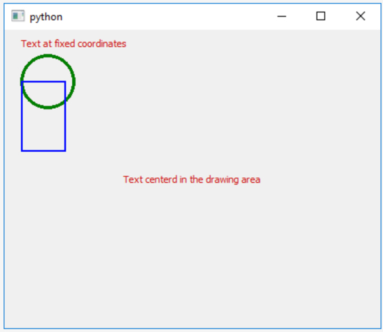
Let’s look at the coarse structure first: we are defining a new class derived from QWidget and only overriding the paintEvent(…) method, meaning in all other aspects this widget will behave like an instance of QWidget. In the main code, we simply create an instance of our new widget class and make it show up on the screen. Now, let’s look at the body of method paintEvent(…): The first thing to note here is that all drawing needs to be preceded by the creation of the QPainter object (line 8) and the call of its begin(…) method using “self” as the parameter standing for the widget object itself because that is what we want to draw on (line 9). To conclude the drawing, we need to call the end() method of the QPainter object (line 19).
Next, let us look at the methods of the QPainter object we are invoking that all start with “draw…”. These are the methods provided by QPainter to draw different kinds of entities like text, circles or ellipses, rectangles, images, etc. We here use the method drawText(…) twice to produce the two different lines of text (lines 12 and 13). The difference between the two calls is that in the first one we use absolute coordinates, so the text will be drawn at pixel coordinates 20, 20 counting from the top left corner of the widget’s content area. The second call takes a rectangle (class QRectF) as the first parameter and then draws the text within this rectangle based on the additional text options given as the second parameter which here says that the text should be centered within the rectangle. This is an example where a class provides several methods with the same name but different parameters, something that is called overloading. If you check out the documentation of QPainter [36], you will see that most methods come in different versions. Now go ahead and resize the window a bit and see how the text produced by the first call always remains at the same absolute position, while that from the second call always stays centered within the available area.
In line 15, we use the method drawEllipse(…) to produce the circle. There is no special circle drawing method, so we use this one and then provide the same number for the two radii. To draw the rectangle, we use the method drawRect(…) in the version that takes the coordinates of the corner plus width and height values as parameters.
The remaining calls of methods of the QPainter object are there to affect the way the objects are drawn, e.g. their color. Colors inPyQt5 are represented by instances of the class QColor. In line 11, we create a new QColor object by providing values between 0 and 255 for the color’s red, green, and blue values. Since the red value is 200 and both green and blue are zero, the overall color will be the kind of red that the text appears in. QT5 also has a number of predefined colors that we are using in lines 14 (Qt.darkGreen) and 16 (Qt.blue).
QPainter uses objects of class QPen [37] and QBrush [38] to draw the boundary and inside of a shape. In line 11, it is stated that a pen with red color should be used for the following drawing operations. As a result, both text lines appear in red. In line 14, we create a new QPen object to be used by the QPainter and specify that the color should be dark green, and the line width should be 4. This is used for drawing the circle. In line 16, we do the same with color blue and line width 2, and, in addition, we say that sharp corners should be used for the connection between to adjacent line segments of the shape’s border. This is used for drawing the rectangle. We won’t go further into the details of the different pen and brush properties here but the documentation of the QPen and QBrush classes provides some more examples and explanations. In addition, you will see more use cases in the walkthrough in the next section.
4.9.2 Adapting the geometry example
We are now going to revist the geometry example we saved in Section 4.8.
To prepare our geometry classes to be drawn on the screen, we first need to modify their definitions by
- introducing the new “color” instance variable for storing a QColor object,
- defining a method called “paint” for drawing the respective object on a screen. This method will have one parameter called “painter” for passing an object of the QPainter class that can be used for drawing onto the widget.
As an exercise, think about where in the class hierarchy you would need to make changes to address points (1) and (2). Once you have thought about this for a bit, read on.
The new attribute “color” is something that all our geometry classes have in common. Therefore, the best place to introduce it is in the root class Geometry. In all subclasses (Circle, Rectangle, Square), you then only have to adapt the constructor to include an additional keyword parameter for the color. Regarding point (2): As we saw above, drawing a circle or a rectangle requires different methods of the QPainter object to be called with different kinds of parameters specific to the particular geometry type. Therefore, we define the method paint(…) in class Geometry but then override it in the subclasses Circle and Rectangle. For class Square, the way it is based on class Rectangle allows us to directly use the implementation of paint(…) from the Rectangle class, so we do not have to override the method in the definition of Square. Here are the changes made to the four classes.
Class Geometry: as discussed, in class Geometry we introduce the “color” variable, so we need to change the constructor a bit. In addition, we add the method paint(…) but without an implementation. The rest of the definition remains unchanged:
class Geometry:

	def __init__(self, x = 0.0, y = 0.0, color = Qt.black):
       	 self.x = x
         self.y = y
         self.color = color

    ...

    def paint(self, painter):
         pass
Classes Circle and Rectangle: for the classes Circle and Rectangle, we adapt the constructors to also include a keyword argument for “color”. The color is directly passed on to the constructor of the base class, while the rest of the constructor remains unchanged. We then provide a definition for method paint(…) that sets up the Pen object to use the right color and then uses the corresponding QPainter method for drawing the object (drawEllipse(…) for class Circle and drawRect(…) for class Rectangle) providing the different instance variables as parameters. The rest of the respective class definitions stay the same:
class Circle (Geometry):

    def __init__(self, x = 0.0, y = 0.0, radius = 1.0, color = Qt.black):
         super(Circle,self).__init__(x,y,color)
         self.radius = radius

    ...

    def paint(self, painter):
         painter.setPen(QtGui.QPen(self.color, 2))
         painter.drawEllipse(QPoint(self.x, self.y), self.radius, self.radius)


class Rectangle(Geometry):

    def __init__(self, x = 0.0, y = 0.0, width = 1.0, height = 1.0, color = Qt.black):
         super(Rectangle,self).__init__(x,y, color)
         self.width = width
         self.height = height

    ...

    def paint(self, painter):
         painter.setPen(QtGui.QPen(self.color, 2,  join = Qt.MiterJoin))
         painter.drawRect(self.x, self.y, self.width, self.height)
Class Square: sor the Square class, we just adapt the constructor to include the color, the rest remains unchanged:
class Square(Rectangle):

    def __init__(self, x = 0.0, y = 0.0, sideLength = 1.0, color = Qt.black):
         super(Square,self).__init__(x, y, sideLength, sideLength, color)
Now that we have the geometry classes prepared, let us again derive a specialized class GeometryDrawingWidget from QWidget that stores a list of geometry objects and in the paintEvent(…) method sets up a QPainter object for drawing on its content area and then invokes the paint(…) methods for all objects from the list. This is bascially the same thing we did towards the end of Section 4.7.2 but now happens inside the new widget class. The list of objects is supposed to be given as a parameter to the constructor of GeometryDrawingWidget:
import math, sys
from PyQt5 import QtGui, QtWidgets
from PyQt5.QtCore import Qt, QPoint

class GeometryDrawingWidget(QtWidgets.QWidget):

     def __init__(self, objects):
         super(GeometryDrawingWidget,self).__init__()
         self.objectsToDraw = objects

     def paintEvent(self, event):
         qp = QtGui.QPainter()
         qp.begin(self)
         for obj in self.objectsToDraw:
             obj.paint(qp)
         qp.end()
Finally, we create another new class called MyMainWindow that is derived from QMainWindow for the main window containing the drawing widget. The constructor takes the list of objects to be drawn and then creates a new instance of GeometryDrawingWidget passing the object list as a parameter and makes it its central widget in line 6:
class MyMainWindow(QtWidgets.QMainWindow):

    def __init__(self, objects):
	    super(MyMainWindow, self).__init__()
	    self.resize(300,300)
	    self.setCentralWidget(GeometryDrawingWidget(objects))
In the main code of the script, we then simply create an instance of MyMainWindow with a predefined list of geometry objects and then call its show() method to make the window appear on the screen:
app = QtWidgets.QApplication(sys.argv)

objects = [ Circle(93,83,45, Qt.darkGreen), Rectangle(10,10,80,50, QtGui.QColor(200, 0, 250)), Square(30,70,38, Qt.blue)]

mainWindow = MyMainWindow (objects)
mainWindow.show()

sys.exit(app.exec_())
When you run the program, the produced window should look like in the figure below. While this is not really visible, every time you resize the window, the paintEvent(…) method of GeometryDrawingWidget will be called and the content consisting of the three geometric objects will be redrawn. While in this simple widget, we only use fixed absolute coordinates so that the drawn content is independent of the size of the widget, one could easily implement some logic that would scale the drawing based on the available space.
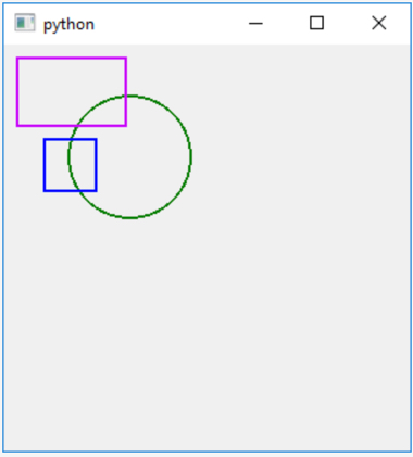
4.10 Walkthrough I: A Bus Track Analyzer for GPS Data of Dublin Buses
It is time to apply what we learned about writing classes, inheritance, and polymorphism in a larger project. In this walkthrough we are going to build an application that processes GPS tracks of buses to detect certain events like a bus being stopped for more than a minute, two buses encountering each other along their routes, etc. Such an application might be used by a public transportation manager to optimize schedules or be warned about irregularities occurring in a real-time tracking data stream. In the walkthrough code, we will be defining classes for real-world objects from the domain like a class Bus, a class Depot, etc. and for abstract concepts like a GPS point with timestamp information and for the events we are looking for. The classes for the different event types we are interested in will be organized into a hierarchy like the geometry classes in section 4.9.
The data we will be using for this project comes from Ireland’s open data portal [39]. The Dublin City Council has published bus GPS data across Dublin City [40] for November 2012 and January 2013 in the form of daily .csv files that list GPS points for active bus vehicles in chronological order with timestamps measured in microseconds since January 1st, 1970. This is a common way of measuring time called Unix or Posix time [41]. GPS measurements for an active vehicle appear in intervals of approximately 20 seconds in the data. The locations are given in WGS84 (EPSG:4326) latitude and longitude coordinates.
We extracted the bus data for 1.5 hours in the late evening of January 30 and morning of January 31, 2013 and cleaned it up a bit, filtering out some outliers and vehicles for which there were only a very small number of GPS points. We manually created a second input file with bounding box coordinates for a few bus depots in Dublin that we will need for detecting certain events and then combined the two input files with some other resources that we will need for this project and the actual source code consisting of several Python .py files. Please download the resulting .zip file [42] and extract it into a new folder.
Have a quick look at the file dublin_bus_data.csv containing the bus GPS points. We are mainly interested in column 1 that contains the time information, column 6 that contains the ID of the bus vehicle, and columns 9 and 10 that contain the latitude and longitude coordinates. We will also use column 2 that contains the number of the line this bus belongs to, but only for information display.
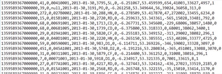
The file dublin_depots.csv contains the bus depot information with columns for the depot name and latitude-longitude pairs for the bottom left and top right corners of the bounding box as a rough approximation of the depot’s actual location and area.
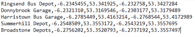
In this walkthrough, we will focus on writing the code for the main classes needed for reading in the data, processing the data and detecting the events, and producing output vector data sets with the bus tracks and detected events. In addition, we will create a QT widget that displays the status of the different buses while the data is being processed. In the following optional part (Sections 4.11 and 4.12), we will further develop this project into a QGIS plugin that includes this widget and shows developing bus trajectories and detected events live as developing layers on the QGIS map canvas.
4.10.1 File and Class Structure of the Project
Since this project involves quite a bit of code, we have tried to cleanly organize it into different class definitions and multiple files. We don’t expect you to type in the code yourself in this walkthrough but rather study the files carefully and use the explanations provided in this text to make sure you understand how everything plays together. Here is an overview on what each of the involved files contains:
core_classes.py – This file contains most of the basic classes for our project that are not derived from other classes.
- class Timepoint: a Timepoint in this project will represent a point in space and time and is therefore defined by latitude and longitude properties which are both instance variables of type float and a time property that is an instance of the class datetime from the datetime module of the Python standard library (that you worked with in homework assignment 3). We will use Timepoints to represent the bus observations from the GPS data as well as events happening at a particular location at a particular time.
- class Bus: the class Bus represents a single vehicle appearing in the GPS data and its GPS points extracted from the input data. It is defined by its vehicle ID, the line it belongs to, and a list of chronologically-ordered Timepoints representing the GPS observation points read from the input data.
- class BusTracker: this class represents the current status of an individual bus vehicle during the analysis and event detection process. A BusTracker object will be maintained for each bus vehicle. It links to the corresponding object of class Bus and, in addition, is used to keep track of whether the vehicle’s status is currently “driving”, “stopped”, or “in depot”, of its current speed estimate, of the last Timepoint that has already been processed for this bus, and of some other information.
- class Observation: in the analysis stage of our program, we will maintain a priority queue (Section 4.2.3) in which we store the next observations for each bus. These observations need to be processed in order of their time of occurrence. The objects we are storing in this queue will be of class Observation that combines the BusTracker for the bus this observation is about, the Timepoint of this observation, and the index of that Timepoint in the list of Timepoints of the bus. Please note that the class has to define its own __lt__(...) method for the < comparison operator to achieve that the Obervation objects in the priority queue will be ordered based on their time attribute of the Timepoint object they contain.
- class Depot: the class Depot is used to represent a single bus depot, simply defined by its name and bounding box which is represented as a 4-tuple of floats as in the original input data in file dublin_depots.csv.
bus_events.py - This file defines the hierarchy of bus events starting with the abstract root class BusEvent from which we derive three more specialized (but still abstract) classes SingleBusEvent, MultipleBusesEvent, and BusDepotEvent. The classes for the events that we are actually trying to detect in the data are derived from these three intermediate classes. The overall bus event hierarchy is depicted in the figure below. We are keeping things somewhat simple here. One could certainly imagine other kinds of events that could be of interest and easily added to this hierarchy.
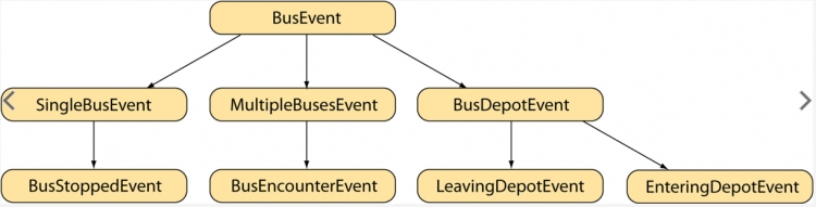
- class BusEvent: each bus event has an associated Timepoint. Therefore, the instance variable for this Timepoint object is already introduced in the abstract root class BusEvent. In addition, each bus event should have a method description() to produce a string with a brief description of the event suitable to be stored in an attribute table of a feature class, and a class function (Section 4.8) called detect(…) that takes an object of class Observation and checks whether the respective event occurs at this observation point and if so, creates and returns one or multiple event objects of that event class. We define templates for both these functions in BusEvent but they need to be overwritten by the derived subclasses.
- class SingleBusEvent: this class is intended as a superclass for all events involving just a single bus, so those that are entirely based on properties of the bus and its GPS data. The class adds an instance variable to refer to the Bus object this event is about.
- class MultipleBusesEvent: this class is the superclass for all bus events that involve two or more buses (like bus encounter events). It adds an instance variable for storing a list of Bus objects, namely those involved in the particular event.
- class BusDepotEvent: all event classes that involve a single bus and a bus depot are supposed to be derived from this intermediate class. It adds instance variables for the involved bus (class Bus) and involved depot (class Depot).
- class BusStoppedEvent: this is the first instantiable class in our hierarchy and it is derived from the SingleBusEvent class because it is only about the properties of an individual bus: when the given Timepoint on the bus doesn’t move more than 3 meters for at least a minute, we consider the bus to be stopped, generate an event of this class, and update the status of the BusTracker for this bus accordingly. This all happens in the function detect(…) that is overwritten in the definition of class BusStoppedEvent. This class adds another instance variable called duration for keeping track of how long the bus remained stopped.
- class BusEncounterEvent: this event derived from class MultipleBusesEvent represents situations in which two buses encounter each other along their routes. The detect(…) function overwritten in the class definition creates an event of this class if the given bus is observed within 20 meters of the last accounted position of another bus while both buses are “driving” (so not stopped and not currently in a depot).
- class LeavingDepotEvent: this class is derived from BusDepotEvent and an event of this class will be generated (again by the overwritten function detect(…)) if the bus still has the status “in depot” but for the given observation now is located outside any depot. The status of the corresponding BusTracker will be changed from “in depot” to “driving”.
- class EnteringDepotEvent: this is the counter part to LeavingDepotEvent for when a bus that still has the status “driving” now for the current observation is located inside one of the depots.
bus_track_analyzer.py – This file contains just a single class definition, the definition of class BusTrackAnalyzer that is our main class for performing the analysis and event detection over the data read in from the two input files. Its constructor takes two input parameters: a dictionary that maps a bus vehicle ID to the corresponding object of class Bus (created from the data from the GPS input file) and a list of Depot objects (created from the data in the depot input file). While its code could also have become the main program for this project, it is advantageous to have this all encapsulated into a class definition with methods for performing a single step of the analysis, resetting the analysis to start from the beginning, and for producing output vector data sets of the bus tracks created and the events detected so far. This way we can use this analyzer differently in different contexts and have full control over when and in which order the individual analysis steps and other actions will be performed. When we turn the project into a QGIS plugin in Section 4.12, we will make use of this by linking the methods of this class to a media player like control GUI with buttons for starting, pausing, and resetting the analysis. We will explain how this main class of the project works in more detail in a moment.
bus_tracker_widget.py – This file also defines just a single class, BusTrackerWidget, which is for visualizing the current status of the buses during the analysis and, therefore, is a bit of an optional component in this project to practice what you learned about drawing on a widget some more in this lesson. A BusTrackerWidget object is directly linked to a BusTrackAnalyzer object that is given to it as a parameter to the constructor. Whenever the content is supposed to be drawn, it accesses the analyzer object and, in particular, the list of BusTracker objects maintained there and depicts the status of the different buses as shown in the image below with each line representing one of the buses:
The class uses the three images from the files status_driving.png, status_indepot.png, and status_stopped.png to show the current status as an icon in the leftmost column of each row. This is followed by a colored circle depicting the vehicles current estimated speed using red for speeds below 15 mph, orange below 25 mph, yellow below 40 mph, and green for speeds larger than 40 mph. Then it displays the bus ID and line information followed by a short text description providing more details on the status like the exact speed estimate or the name of the depot the bus is currently located in. The widget also shows the time of the last processed observation in green at the top. We will discuss how this class has been implemented in more detail later in this section.
main.py – Lastly, this file contains the main program for this project in which we put everything together. Since most of the analysis functionality is implemented in class BusTrackAnalyzer and the detect(…) functions of the different bus event classes, this main program is comparatively compact. It reads in the data from the two input files, creates a BusTrackAnalyzer for the resulting Bus and Depot objects, and sets up a QWidget for a window that hosts an instance of the BusTrackerWidget class. When the main button in this QWidget is pressed, the run method is executed and processes the data step-by-step by iteratively calling the nextStep() method of the analyzer object until all observations have been processed. The method also makes sure that the BusTrackerWidget is repainted after each step so that we can see what is happening during the analysis. Finally, it saves the detected events and bus tracks as vector data sets on the disk.
4.10.2 Implementation Details
Now that you have a broad overview of the classes and files involved, let’s look at the code in more detail. The code is too long to explain every line and there are parts that should be easy to understand with the knowledge you have now and the comments included in the source code, so we will only be picking out the main points. Nevertheless, please make sure to study carefully the class definitions and how they work together, and if something is unclear, please ask on the forums.
4.10.2.1 Reading the Input Data
To study the interplay between the classes and implementation details, let us approach things in the order in which things happen when the main program in main.py is executed. After the main input variables like the paths for the two input files and a dictionary for the indices of the columns in the GPS input file have been defined in lines 15 to 21 of main.py, the first thing that happens is that the data is read in and used to produce objects of classes Bus and Depot for each bus vehicle and depot mentioned in the two input files.
The reading of the input data happens in lines 24 and 25 of main.py.
depotData = Depot.readFromCSV(depotFile)
busData = Bus.readFromCSV(busFile, busFileColumnIndices)
Both classes Bus and Depot provide class functions called readFromCSV(...) that given a filename read in the data from the respective input file and produce corresponding objects. For class Depot this happens in lines 112 to 120 of core_classes.py and the return value is a simple list of Depot objects created in line 119 with given name string and 4-tuple of numbers for the bounding box.
def readFromCSV(fileName):
         """reads comma-separated text file with each row representing a depot and returns list of created Depot objects.
            The order of columns in the file is expected to match the order of parameters and bounding box elements of the Depot class."""
         depots = []
         with open(os.path.join(os.path.dirname(__file__), fileName), "r") as depotFile:
             csvReader = csv.reader(depotFile, delimiter=',')
             for row in csvReader:                 # go through rows in input file
                 depots.append(Depot(row[0], (float(row[1]),float(row[2]),float(row[3]),float(row[4]))))  # add new Depot object for current row to Depot list
         return depots
For class Bus, this happens in lines 20 to 49 of core_classes.py and is slightly more involved. It works somewhat similarly to the code from the rhino/race car project in lesson 4 of GEOG485 in that it uses a dictionary to create Timepoint lists for each individual bus vehicle occurring in the data.
def readFromCSV(fileName, columnIndices):
        """reads comma-separated text file with each row representing a GPS point for a bus with timestamp and returns dictionary mapping
           bus id to created Bus objects. The column indices for the important info ('lat', 'lon', 'time', 'busID', 'line') need to be
           provided in dictionary columnIndices."""
        buses = {}

        with open(os.path.join(os.path.dirname(__file__), fileName), "r") as trackFile:
            csvReader = csv.reader(trackFile, delimiter=',')
            for row in csvReader:
                # read required info from current row
                busId = row[columnIndices['busId']]
                lat = row[columnIndices['lat']]
                lon = row[columnIndices['lon']]
                time = row[columnIndices['time']]
                line = row[columnIndices['line']]

                # create datetime object from time; we here assume that time in the csv file is given in microseconds since January 1, 1970
                dt = datetime.datetime(1970, 1, 1) + datetime.timedelta(microseconds=int(time))

                # create and add new Bus object if this is the first point for this bus id, else take Bus object from the dictionary
                if not busId in buses:
                    bus = Bus(busId, line)
                    buses[busId] = bus
                else:
                    bus = buses[busId]

                # create Timepoint object for this row and add it to the bus's Timepoint list
                bus.timepoints.append(Timepoint(dt,float(lat),float(lon)))

        	return buses  # return dictionary with Bus objects created
For each row in the csv file processed by the main for-loop in lines 28 to 47, we extract the content of the cells we are interested in, create a new datetime object based on the timestamp in that row, and then, if no bus with that ID is already contained in the dictionary we are maintaining in variable buses, meaning that this is the first GPS point for this bus ID in the file, we create a new Bus object and put it into the dictionary using the bus ID as the key. Else we keep working with the Bus object we have already stored under that ID in the dictionary. In both cases, we then add a new Timepoint object for the data in that row to the list of Timepoints kept in the Bus object (line 47). The dictionary of Bus objects is returned as the return value of the function. Having all Timepoints for a bus nicely stored as a list inside the corresponding Bus object will make it easy for us to look ahead and back in time to determine things like current estimated speed and whether the bus is stopped or driving at a particular point in time.
4.10.2.2 Setting up the BusTrackAnalyzer
Next, we create the BusTrackAnalyzer object to be used for the event detection in line 28 of main.py providing the bus dictionary and depot list as parameters to the constructor together with a list of class names for the bus event classes that we want the analyzer to detect. This list is defined in line 17 of main.py.
eventClasses = [ LeavingDepotEvent, EnteringDepotEvent, BusStoppedEvent, BusEncounterEvent ] # list of event classes to detect

...


# create main BusTrackAnalyzer object
analyzer = BusTrackAnalyzer(busData, depotData, eventClasses)
If you look at lines 12 to 21 of bus_track_analyzer.py, you will see that the constructor takes these parameters and stores them in its own instance variables for performing analysis steps later on (lines 16, 17 and 19).
def __init__(self, busData, depotData, eventClasses):
         self.allBusTrackers = []            # list of BusTracker objects for all buses currently being processed
         self.allEvents = []                 # used for storing all Event objects created during an analysis run
         self.lastProcessedTimepoint = None  # Timepoint of the last Observation that has been processed
         self._busData = busData             # dictionary mapping bus Id strings to Bus objects with GPS data
         self._depotData = depotData         # list of Depot objects used for Event detection
         self._observationQueue = []         # priority queue of next Observation objects to be processed for each bus
         self._eventClasses = eventClasses   # list of instantiable subclasses of BusEvent that should be detected

         self.reset()   # initialize variables for new analysis run
In addition, the constructor sets up some more instance variables that will be needed when the analysis is run: a list of bus trackers (one for each bus) in variable allBusTrackers, a list of events detected in variable allEvents, a variable lastProcessedTimepoint for the Timepoint of the last observation processed, and a list in variable _observationQueue that will serve as the priority queue of Observation objects to be processed next. Then in the last line, we call the method reset() of BusTrackAnalyzer defined in lines 23 to 40 whose purpose is to reset the value of these instance variables to what they need to be before the first analysis step is performed, allowing the analysis to be reset and repeated at any time.
def reset(self):
         """reset current analysis run and reinitialize everything for a new run"""
         self.allBusTrackers = []
         self.allEvents = []
         self.lastProcessedTimepoint = None
         self._observationQueue = []

         for busId, bus in self._busData.items():  # go through all buses in the data
             busTracker = BusTracker(bus)          # create new BusTracker object for bus

             # set initial BusTracker status to "IN DEPOT" if bus is inside bounding box of one of the depots
             isInDepot, depot = Depot.inDepot(bus.timepoints[0].lat, bus.timepoints[0].lon, self._depotData)
             if isInDepot:
                 busTracker.status = BusTracker.STATUS_INDEPOT
                 busTracker.depot = depot

             self.allBusTrackers.append(busTracker) # add new BusTracker to list of all BusTrackers
             heapq.heappush(self._observationQueue, Observation(busTracker, 0)) # create Observation for first Timepoint of this bus
                                                                                # and add to Observation priority queue
The main thing the method does is go through the dictionary with all the Bus objects and, for each, create a new BusTracker object that will be placed in the allBusTrackers list, set the initial status of that BusTracker to STATUS_INDEPOT if the first Timepoint for that bus is inside one of the depots (else the status will be the default value STATUS_DRIVING), and create an Observation object with that BusTracker for the first Timepoint from the Timepoint list of the corresponding bus that will be put into the observation priority queue via the call of the heapq.headpush(…) function (line 40). The image below illustrates how the main instance variables of the BusTrackAnalyzer object may look after this initialization for an imaginary input data set.
The buses with IDs 5, 2145, and 270 are the ones with earliest GPS observations in our imaginary data but there can be more busses that we are not showing in the diagram. We are also not showing all instance variables for each object, just the most important ones. Furthermore, Timepoint objects are shown as simple date + time values in the diagram not as objects of class Timepoint. The arrows indicate which objects the different instance variables contain starting with the _observationQueue, allBusTrackers, and allEvents instance variables of the single BusTrackAnalyzer object that we have.
The Bus objects at the top that contain the GPS data read from the input file will not change anymore and we are not showing here that these are actually maintained in a dictionary. The list of BusTracker objects (one for each Bus object) will also not change anymore but the properties of the individual BusTracker objects in it will change during the analysis. The observation queue list is the one that will change the most during the analysis because it will always contain the Observation objects to be processed ordered by the time point information. The event list is still empty because we have not detected any events yet.
4.10.2.3 Running the Analysis
The method nextStep() defined in lines 47 to 71 of bus_track_analyzer.py is where the main work of running a single step in the analysis, meaning processing a single observation, happens. In addition, the class provides a method isFinished() for checking if the analysis has been completed, meaning there are no more observations to be processed in the observation priority queue. Let us first look at how we are calling nextStep() from our main program:
    def run(self):
        """performs only a single analysis step of the BusTrackAnalyzer but starts a timer after each step to call the function again after a
           brief delay until the analzzer has finished. Then saves events and bus tracks to GeoPackage output files."""
        mainWidget.button.setEnabled(False) # disable button so that it can't be run again
        if not analyzer.isFinished():       # if the analyzer hasn't finished yet, perform next step, update widget, and start timer
                                            # to call this function again
            analyzer.nextStep()
            mainWidget.busTrackerWidget.updateContent()
            timer = QTimer()
            timer.singleShot(delay, self.run)
        else:                               # when the analyzer has finished write events and bus tracks to new GeoPackage files
            analyzer.saveBusTrackPolylineFile("dublin_bus_tracks.gpkg", "GPKG")
            analyzer.saveEventPointFile("dublin_bus_events.gpkg",  "GPKG")

            # reset analyzer and enable button again
            analyzer.reset()
            mainWidget.button.setEnabled(True)
The method run() in lines 47 to 63 of main.py is called when the “Run” button of our main window for the program is clicked. This connection is done in line 45 of main.py:
self.button.clicked.connect(self.run)
The idea of this method is that unless the analysis has already been completed, it calls nextStep() of the analyzer object to perform the next step (line 53) and then in lines 55 and 56 it starts a QT timer that will invoke run() again once the timer expires. That means run() will be called and executed again and again until all observations have been processed but with small delays between the steps whose length is controlled by variable delay defined in line 21. This gives us some control over how quickly the analysis is run allowing us to observe the changes in the BusTrackerWidget in more detail by increasing the delay value. To make this approach safe, the method first disables the Run button so that the timer is the only way the function can be invoked again.
Now let’s look at the code of nextStep() in more detail (lines 47 to 71 of bus_track_analyzer.py):
	def nextStep(self):
         """performs next step by processing Observation at the front of the Observations priority queue"""
         observation = heapq.heappop(self._observationQueue)           # get Observation that is at front of queue

         # go through list of BusEvent subclasses and invoke their detect() method; then collect the events produced
         # and add them to the allEvents lists
         for evClass in self._eventClasses:
             eventsProduced = evClass.detect(observation, self._depotData, self.allBusTrackers) # invoke event detection method
             self.allEvents.extend(eventsProduced)  # add resulting events to event list

         # update BusTracker of Observation that was just processed
         observation.busTracker.lastProcessedIndex += 1
         observation.busTracker.updateSpeed()

         if observation.busTracker.status == BusTracker.STATUS_STOPPED: # if  duration of a stopped event has just expired, change status to "DRIVING"
             if observation.timepoint.time > observation.busTracker.statusEvent.timepoint.time + observation.busTracker.statusEvent.duration:
                 observation.busTracker.status = BusTracker.STATUS_DRIVING
                 observation.busTracker.statusEvent = None

         # if this was not the last GPS Timepoint of this bus, create new Observation for the next point and add it to the Observation queue
         if observation.timepointIndex < len(observation.busTracker.bus.timepoints) - 1:  # not last point
             heapq.heappush(self._observationQueue, Observation(observation.busTracker, observation.timepointIndex + 1)  )

         # update analyzer status
         self.lastProcessedTimepoint = observation.timepoint
The code is actually simpler than one might think because the actual event detection is done in the bus event classes. The method does the following things in this order:
- Take next observation from queue: it takes the Observation object at the front of the _observationQueue priority queue out of the queue (line 49). This is the observation with the earliest timestamp that still needs to be processed. Remember that the Observation object consists of a BusTracker object and the observation Timepoint and its index.
- Call detect() function for all event classes: the method then goes through the list of event classes that contains the names of the four event classes making up the bottom level in our bus event hierarchy (see Figure 4.23 from Section 4.10.1 [43]) and for each calls the corresponding detect(…) class function (line 54) passing the Observation object as well as the list of depots and the list of all BusTracker objects as parameters, so that the event detection has all the information needed to decide whether an event of this kind is occurring for this observation. The event objects produced and returned as a list from calling detect(…) are then added to the list in allEvent (line 55).
- Update BusTracker: next, the BusTracker object for the current observation is updated to reflect that this Timepoint has been processed and we call its updateSpeed(…) method to compute a new speed estimate based on the current, previous, and next Timepoints for that bus. The code for this method can be found in lines 67 to 81 of core_classes.py and it uses the geopy function great_circle(…) to compute the distance between two WGS84 points. Since our bus event hierarchy does not include an event for when a stopped bus starts to move again, we need some place to change its BusTracker status to STATUS_DRIVING when this happens. This is done in lines 61 to 64 of this method.
- Put next Observation for this bus into queue: unless this observation was for the last Timepoint from the list of Timepoints for that bus, we now generate a new Observation object with the same BusTracker but for the next Timepoint from the Timepoints list and put this Observation into the priority queue (line 68). Since the queue is always kept sorted by observation time, it is guaranteed that all bus observation will be processed in the correct chronological order.
- Update analyzer status: finally, the lastProcessedTimepoint variable of the analyzer itself is updated to always provide the Timepoint of the last Observation processed (line 71).
To illustrate this process, let’s imagine we run the first analysis step for the initial situation from Section 4.10.2.2 with a bus that is not in one of the depots but is nevertheless stopped at the moment. The first Obervation object taken from the queue in step (1) then contains the BusTracker for the bus with ID 2145 and the Timepoint 2013/1/30 23:45:00.
In step(2), we first invoke the detect(…) function of the LeavingDepotEvent class because that is the first class appearing in the list. The code for this function can be found in lines 122 to 140 of bus_events.py.
def detect(observation, depots, activeBusTrackers):
        """process observation and checks whether this event occurs at the given observation. If yes, one or more instances of
           this Event class are created and returned as a list."""
        producedEvents = [] # initialize list of newly created events to be returned by this function

        if observation.busTracker.status == BusTracker.STATUS_INDEPOT:
            isInDepot, depot = Depot.inDepot(observation.timepoint.lat, observation.timepoint.lon, depots)  # test whether bus is still in a depot
            if not isInDepot: # bus not in depot anymore, so leaving depot event will be created and added to result list
                event =  LeavingDepotEvent(observation.timepoint, observation.busTracker.bus, observation.busTracker.depot)
                producedEvents.append(event)
                observation.busTracker.status = BusTracker.STATUS_DRIVING  # update BusTracker object to reflect detected new status
                observation.busTracker.statusEvent = None
                observation.busTracker.depot = None
                print("Event produced:", str(event))

        else:
            pass # nothing to do if bus is not in depot

        return producedEvents
The first thing tested there is whether or not the current status of the BusTracker is STATUS_INDEPOT which is not the case. Hence, we immediately return from that function with an empty list as the return value. If instead the condition would have been true, the code of this function would have checked whether or not the bus is currenctly still in a depot by calling the Depot.inDepot(...) function (line 128). If that would not be the case, an event object of this class would be created by calling the LeavingDepotEvent(...) constructor (line 130) and the status information in the corresponding BusTracker object would be updated accordingly (lines 132-135). The created LeavingDepotEvent object would be added to the list in variable producedEvents (line 131) that is returned when the end of the function is reached.
Next, this step is repeated with the detect(…) function from EnteringDepotEvent defined in lines 152 to 170 of bus_events.py. The condition that the bus should currently be driving is satisfied, so the code next checks whether or not the current position of the bus given by observation.timepoint.lat and observation.timepoint.lon (line 158) is inside one of the depots by calling the function inDepot(…) defined as part of the class definition of class Depot in lines 104 to 110 of core_classes.py. This is not the case, so again an empty event list is returned.
Next, detect(…) of the class BusStoppedEvent is called. This is most likely the most difficult to understand version of the detect(…) functions and it can be found in lines 35 to 65 of bus_events.py:
def detect(observation, depots, activeBusTrackers):
         """process observation and checks whether this event occurs at the given observation. If yes, one or more instances of
            this Event class are created and returned as a list."""
         producedEvents = []  # initialize list of newly created events to be returned by this function

         if observation.busTracker.status == BusTracker.STATUS_DRIVING:
             # look ahead until bus has moved at least 3 meters or the end of the Timepoint list is reached
             timeNotMoving = datetime.timedelta(seconds=0) # for keeping track of time the bus hasn't moved more than 3 meters
             distance = 0 # for keeping track of distance to original location
             c = 1 # counter variable for looking ahead
             while distance < 3 and observation.timepointIndex  + c < len(observation.busTracker.bus.timepoints):
                 nextTimepoint =  observation.busTracker.bus.timepoints[observation.timepointIndex  + c] # next Timepoint while looking ahead
                 distance = great_circle( (nextTimepoint.lat, nextTimepoint.lon), (observation.timepoint.lat, observation.timepoint.lon) ).m # distance to next Timepoint

                 if distance < 3:  # if still below 3 meters, update timeNotMoving
                     timeNotMoving = nextTimepoint.time - observation.timepoint.time

                 c += 1

             # check whether bus didn't move for at least 60 seconds and if so generate event
             if timeNotMoving.total_seconds() >= 60:
                 event =  BusStoppedEvent(observation.timepoint, observation.busTracker.bus, timeNotMoving)    # create stopped event
                 producedEvents.append(event)     # add new event to result list
                 observation.busTracker.status = BusTracker.STATUS_STOPPED    # update BusTracker object to reflect detected stopped status
                 observation.busTracker.statusEvent = event
                 print("Event produced: ", str(event))

         else:
             pass # no stop event will be created while bus status is "IN DEPOT" or "DRIVING"

         return producedEvents
The condition is again that the current BusTracker status is “driving” which is satisfied. The code will then run a while-loop that looks at the next Timepoints in the list of Timepoints for this bus until the distance to the current position gets larger than 3 meters. In this case, this only happens for the fifth Timepoint following the current Timepoint. The code then looks at the time difference between these two Timepoints (line 55) and if its more than 60 second, like in this case, creates a new object of class BusStoppedEvent (line 56) using the current Timepoint, Bus object from the BusTracker, and time difference to set the instance variables of the newly created event object. This event object is put into the event list that will be returned by the detect(…) function (line 57). Finally, the status of the BusTracker object involved will be changed to “stopped” (line 58) and we also store the event object inside the BusTracker to be able to change the status back to “driving” when the duration of the event is over (line 59). When we return from the detect(…) function, the produced BusStoppedEvent will be added to the allEvents list of the analyzer (line 55 of bus_track_analyzer.py).
Finally, detect(…) of BusEncounterEvent will be called, the last event class from the list. If you look at lines 83 to 102 of bus_events.py, you will see that a requirement for this event is that the bus is currently “driving”. Since we just changed the status of the BusTracker to “stopped” this is not the case and no events will be generated and returned from this function call. Just to emphasize this again, the details of how the different detect(...) functions work are less important here; the important thing to understand is that we are using the detect(...) functions defined in each of the bottom level bus event classes to test whether or not one (or even multiple) event(s) of that type occurred and if so generate an event object of that class with information describing that event by calling the constructor of the class (e.g., BusStoppedEvent(...)). Each created event object is added to the list that the detect(...) function returns to the calling nextStep(...) function. In the lesson's homework assignment you will have to use a similar approach but within a much less complicated project.
Now steps (3) –(6) are performed with the result that the lastProcessedIndex of the BusTracker is increased by one (to 1), a new estimated speed is computed for it, a new observation is created for bus 2145 and added to the queue, now for time point 2013/1/30 23:45:03. Since the first observation for bus 270 only has a timestamp of 23:45:05, the new Observation is inserted into the queue in second place after the first Observation for the bus with busId 5. Finally, the lastProcessedTimepoint of the analyzer is changed to 2013/1/30 23:45:00. The resulting constellation after this first run of nextStep() is shown in the image below.
We have intentionally placed some print statements inside the bus event classes from bus_events.py whenever a new event of that class is detected and a corresponding object is created. Normally you wouldn’t do that but here we want to keep track of the events produced when running the main program. So test out the program by executing main.py (e.g., from the OSGeo4W shell after running the commands for setting the environment variables as described in Section 4.4.1) and just look at the output produced in the console, while still ignoring the graphical output in the window for a moment.
The produced output will start like this but list quite a few more bus events detected during the analysis:
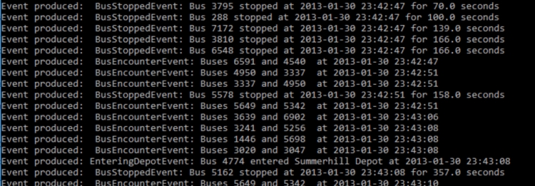
4.10.2.4 Producing the output GPGK files
Remember that we said that the code from main.py will also produce output vector data sets of the bus tracks and events in the end. This happens in lines 57 to 63 of main.py which are only executed when analyzer.isFinished() returns True, so when the analysis has processed all observations:
        else:                               # when the analyzer has finished write events and bus tracks to new GeoPackage files
            analyzer.saveBusTrackPolylineFile("dublin_bus_tracks.gpkg", "GPKG")
            analyzer.saveEventPointFile("dublin_bus_events.gpkg",  "GPKG")

            # reset analyzer and enable button again
            analyzer.reset()
            mainWidget.button.setEnabled(True)
This code assumes that the QGIS environment has already been set up which happens in lines 69 to 73 of main.py; this code should look familiar from Section 4.5.3. The code for creating the output files can be found in the two methods saveBusTrackPolylineFile(…) and saveEventPointFile(…) of BusTrackAnalyzer in lines 73 to 114 of bus_track_analyzer.py.
def saveBusTrackPolylineFile(self, filename, fileFormat):
         """save event list as a WGS84 point vector dataset using qgis under the provided filename and using the given format. It is
            expected that qgis has been initalized before calling this method"""
         # create layer for polylines in EPSG:4326 and an integer field BUS_ID for storing the bus id for each track
         layer = qgis.core.QgsVectorLayer('LineString?crs=EPSG:4326&field=BUS_ID:integer', 'tracks' , 'memory')
         prov = layer.dataProvider()

         # create polyline features
         features = []
         for busId, bus in self._busData.items():
             # use list comprehension to produce list of QgsPoinXY objects from bus's Timepoints
             points = [ qgis.core.QgsPointXY(tp.lon,tp.lat) for tp in bus.timepoints ]
             feat = qgis.core.QgsFeature()
             lineGeometry = qgis.core.QgsGeometry.fromPolylineXY(points)
             feat.setGeometry(lineGeometry)
             feat.setAttributes([int(busId)])
             features.append(feat)

         # add features to layer and write layer to file
         prov.addFeatures(features)
         qgis.core.QgsVectorFileWriter.writeAsVectorFormat( layer, filename, "utf-8", layer.crs(), fileFormat)
saveBusTrackPolylineFile(…) creates a list of QgsPointXY objects from the Timepoints of each Bus object (line 105) and then creates a Polyline geometry from it (line 107) which is further turned into a feature with an attribute for the ID of the bus, and then added to the created layer in line 113. Finally, the layer is written to a new file using the name and format given as parameter to the function. We here use the GeoPackage format “GPKG” but this can easily be changed in main.py to produce, for instance, a shapefile instead.
	def saveEventPointFile(self, filename, fileFormat):
         """save event list as a WGS84 point vector dataset using qgis under the provided filename and using the given format. It is
            expected that qgis has been initalized before calling this method"""
         # create layer for points in EPSG:4326 and with two string fields called TYPE and INFO
         layer = qgis.core.QgsVectorLayer('Point?crs=EPSG:4326&field=TYPE:string(50)&field=INFO:string(255)', 'events' , 'memory')
         prov = layer.dataProvider()

         # create point features for all events from self.allEvents and use their Event class name
         # and string provided by description() method for the TYPE and INFO attribute columns
         features = []
         for event in self.allEvents:
             p =  qgis.core.QgsPointXY(event.timepoint.lon, event.timepoint.lat)
             feat = qgis.core.QgsFeature()
             feat.setGeometry(qgis.core.QgsGeometry.fromPointXY(p))
             feat.setAttributes([type(event).__name__, event.description()])
             features.append(feat)

         # add features to layer and write layer to file
         prov.addFeatures(features)
         qgis.core.QgsVectorFileWriter.writeAsVectorFormat( layer, filename, "utf-8", layer.crs(), fileFormat)
saveEventPointFile(…) works in the same way but produces QgsPointXY point features with the attribute fields TYPE and INFO for each event in the allEvents list. The TYPE field will contain the name of the event class this event is from, and the INFO field will contain the short description produced by calling the description() method of the event. Notice this just needs a single line (line 87) because of our event class hierarchy and polymorphism. When opening the two produced files in QGIS, adding a basemap, and adapting the symbology a bit, the result looks like this:
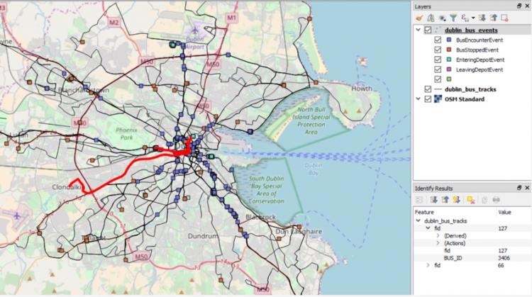
We hope the way this program works got clear from this explanation with (a) the BusTrackAnalyzer being the central class for running the event detection in a step-wise fashion, (b) the Observation objects maintained in a priority queue being used to process the GPS observation in chronological order, (c) the BusTracker objects being used to keep track of the current status of a bus during the analysis, and (d) the different bus event classes all providing their own function to detect whether or not an event of that type has occurred. The program is definitely quite complex but this is the last lesson so it is getting time to see some larger projects and learn to read the source code. As the final step, let's look at the BusTrackerWidget class that provides a visualization of event detection while the analysis process is running.
4.10.2.5 The Bus Tracker Widget for visualizing the analysis process
As we explained before, we also wanted to set up a QT widget that shows the status of each bus tracker while the data is being processed and we implemented the class BusTrackerWidget in bus_tracker_widget.py derived from QWidget for this purpose. In lines 30 to 44 of main.py we are creating the main window for this program and in line 41 we add an instance of BusTrackerWidget to the QScrollArea in the center of that window:
class MainWidget(QWidget):
     """main window for this application containing a button to start the analysis and a scroll area for the BusTrackerWidget"""
     def __init__(self, analyzer):
         super(MainWidget,self).__init__()
         self.resize(300,500)
         grid = QGridLayout(self)
         self.button = QPushButton("Run")
         grid.addWidget(self.button,0,0)
         self.busTrackerWidget = BusTrackerWidget(analyzer) # place BusTrackerWidget for our BusTrackAnalyzer in scroll area
         scroll = QScrollArea()
         scroll.setWidgetResizable(True)
         scroll.setWidget(self.busTrackerWidget)
         grid.addWidget(scroll, 1, 0)

         self.button.clicked.connect(self.run) # when button is clicked call run() function
We are embedding the widget in a QScrollArea to make sure that vertical and horizontal scrollbars will automatically appear when the content becomes too large to be displayed. For this to work, we only have to set the minimum width and height properties of the BusTrackerWidget object accordingly. Please note that in line 53 of main.py we are calling the method updateContent() of BusTrackerWidget so that the widget and its content will be repainted whenever another analysis step has been performed.
Looking at the definition of class BusTrackerWidget in bus_tracker_widget.py, the important things happen in its paintEvent(…) method in lines 24 to 85. Remember that this is the method that will be called whenever QT creates a paint event for this widget, so not only when we force this by calling the repaint() method but also when the parent widget has been resized, for example.
def paintEvent(self, event):
         """draws content with bus status information"""
         # set minimum dimensions basd on number of buses
         self.setMinimumHeight(len(self.analyzer.allBusTrackers) * 23 + 50)
         self.setMinimumWidth(425)

         # create QPainter and start drawing
         qp = QtGui.QPainter()
         qp.begin(self)

         normalFont = qp.font()
         boldFont = qp.font()
         boldFont.setBold(True)

         # draw time of last processed Timepoint at the top
         qp.setPen(Qt.darkGreen)
         qp.setFont(boldFont)
         if self.analyzer.lastProcessedTimepoint:
             qp.drawText(5,10,"Time: {0}".format(self.analyzer.lastProcessedTimepoint.time))
         qp.setPen(Qt.black)

         …
The first thing that happens in this code is that we set the minimum height property of our widget based on the number of BusTracker objects that we need to provide status information for (line 27). For the minimum width, we can instead use a fixed value that is large enough to display the rows. Next, we create the QPainter object needed for drawing (line 31 and 32) and draw the time of the last Timepoint processed by the analyzer to the top of the window (line 42) unless its value is still None.
	# loop through all BusTrackers in the BusTrackAnalyzer
        for index, tracker in enumerate(self.analyzer.allBusTrackers):
          ...
In the main for-loop starting in line 46, we go through the list of BusTracker objects in the associated BusTrackAnalyzer object and produce one row for each of them. All drawing operations in the loop body compute the y coordinate as the product of the index of the current BusTracker in the list available in variable index and the constant 23 for the height of a single row (e.g., 20 +23 * index in line 49 for drawing the bus status icon).
             # draw icon reflecting bus status
    	     qp.drawPixmap(5,20 + 23 * index,self._busIcons[tracker.status])

             # draw speed circles
             color = Qt.transparent
             if tracker.speedEstimate:
                 if tracker.speedEstimate < 15:
                     color = Qt.red
                 elif tracker.speedEstimate < 25:
                     color = QtGui.QColor(244, 176, 66)
                 elif tracker.speedEstimate < 40:
                     color = Qt.yellow
                 else:
                     color = Qt.green
             qp.setBrush(color)
             qp.drawEllipse(80, 23 + 23 * index, 7, 7)
             …
The bus status icon is drawn in line 49 using the drawPixmap(…) method with the QPixmap icon from the _busIcons dictionary for the given status of the bus tracker. Next, the small colored circle for the speed has to be drawn which happens in line 53. The color is determined by the if-elif construct in lines 53 to 61.
             # draw bus id and line text
             qp.setFont(boldFont)
             qp.drawText(100, 32 + 23 * index, tracker.bus.busId + "  [line "+tracker.bus.line+"]")

             # draw status and speed text
             qp.setFont(normalFont)
             statusText = "currently " + tracker.status
             if tracker.status == BusTracker.STATUS_INDEPOT:
                 statusText += " " + tracker.depot.name
             elif tracker.status == BusTracker.STATUS_DRIVING:
                 if not tracker.speedEstimate:
                     speedText = "???"
                 else:
                     speedText  = "{0:.2f} mph".format(tracker.speedEstimate)
                 statusText += " with " + speedText

             qp.drawText(200, 32 + 23 * index, statusText )
Next the bus ID and bus line number are drawn (line 66 and 67). This is followed by the code for creating the status information that contains some case distinctions to construct the string that should be displayed in line 81 in variable statusText based on the current status of the bus.
Now run the program, make the main window as large as possible and observe how the status information in the bus tracker widget is constantly updated like in the brief video below. Keep in mind that you can change the speed this all runs in by increasing the value of variable delay defined in line 21 of main.py. Refresher for running python scripts from the OSGeo4W Shell, you can use python-qgis-ltr, so e.g.
python-qgis-ltr main.py
The video has been recorded with a value of 5. [NOTE: This video (:58) does NOT contain sound.]
After developing the Bus Track Analyzer code as a standalone QGIS based application, we will now turn to the (optional) topic of creating QGIS plugins and how our analyzer code can be turned into a plugin that, as an extension, displays the bus trajectories and detected event live on the QGIS map canvas while the anaylsis is performed.
4.11 Optional: Writing QGIS Plugins
In this section and the next, we are going to demonstrate how to create plugins for QGIS and then turn the Bus Track Analyzer code from the previous walkthrough into a plugin that adds new layers to the current QGIS project and displays the analysis progress live on the map canvas. However, if this lesson has been your first contact with writing classes and your head is swimming a bit with all the new concepts introduced or you are simply running out of time, we suggest that you just briefly skim through these sections and then watch the video from Section 4.12.7 showing the final Bus Track Analyzer for QGIS plugin. While creating a QGIS plugin yourself is one option that would give you full over&above points in this lesson's homework assignment, the content of these two sections is not required for the assignment and the quiz. You can always come back to these sections if you have time left at the end of the lesson or after the end of the class.
In Section 4.5, you already got an idea of how to write Python code that uses the qgis package, and we also made use of this in the walkthrough from the previous section to produce the final output data sets. In this section, we will teach you how to create plugins for QGIS that show up in the plugin manager and can be integrated into the main QGIS GUI.
Instead of programming QGIS plugins from scratch, we will use the Plugin Builder 3 plugin to create the main files needed for us, and then we will modify and complement these to implement the functionality of our plugin. In this section, we will show you the general workflow of creating a plugin using a simple “Random number generator” plugin with only very little actual functionality. In the walkthrough that follows in the next section, we will then apply this approach to create a plugin version of our Bus Track Analyzer tool from the first walkthrough of the lesson.
4.11.1 Creating a Plugin Template with Plugin Builder 3
The plugin builder 3 plugin should already be installed in your QGIS version. If not, please go back to Section 4.4.1 and follow the installation instructions there. Now run the plugin by going Plugins -> Plugin Builder in the main menu.
To create a template for your plugin, you have to work through the dialog boxes of Plugin Builder and fill out the information there. Clicking the “Help” button will open a local .html page with detailed information on the purpose and meaning of the different fields. We fill out the first page as shown in the figure below. Here is a brief overview:
- Class name: this is the name of the main class for our plugin. It needs to be a valid Python class name.
- Plugin name: this is the name of the plugin in readable form. In contrast to the class name, it can contain spaces and other special characters.
- Description: a short description of what the plugin is for.
- Module name: the name of the .py file that will contain the main class for your plugin. Typically, the class name written with underscores rather than in CamelCase is used here.
- Version number & Minimum QGIS version: these are used to specify a version number for your plugin and the minimum QGIS version required to run it.
- Author/Company & Email address: here you provide information about the author of the plugin that will be used to create the copyright information at the beginning of the different files. We have no intentation of publishing this plugin, so we just use “489” here.
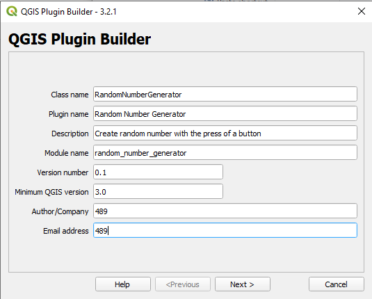
On the next page, you can enter a longer description of your plugin. Since this is just a toy example, we don’t bother with this here and leave the text as it is.
On the next page, you can choose between different kinds of templates for your plugin, e.g. a simple dialog box or a dock widget, meaning an actual panel that can be docked and moved inside the QGIS GUI like the other panels, e.g. the Layers panel. We here will go with the dialog option. In the next section, we will then use the dock widget option. With the “Text for the menu item” option, we specify which text should show up in the menu for our plugin in the main menu bar. With the “Menu” option we pick in which menu of the menu bar this entry should be located. We will fill out this page as shown below:
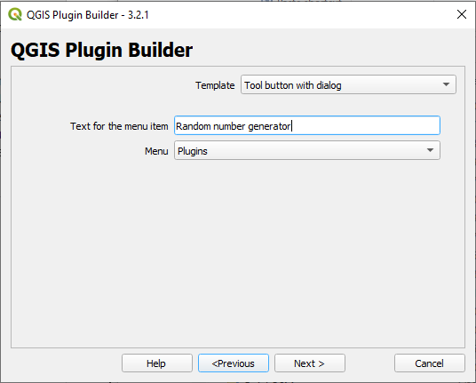
The checkboxes on the next page allow for determining which files Plugin Builder is going to create. It’s ok to leave all options checked.
The next page is specifying information that is relevant if you plan to publish your plugin, e.g. on Github. Since we are not planning this, we just leave the page unchanged.
On the last page, we can determine in which folder the new folder with the files for our plugin will be created. By default this is the default plugin folder of our QGIS installation, meaning the plugin will immediately be listed in QGIS when we start it next. If, instead of the path, you just see a dot (.), please browse to the plugins folder yourself, replacing the part directly after "C:/Users/" with your Windows user name. It is possible that the “AppData” folder in your user’s home directory is not visible in which case you will have to change your settings to show hidden files.
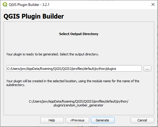
We now click the “Generate” button and Plugin Builder will then create the folder and different files for our plugin. It's possible that you will get a warning message that about Plugin Builder not being able to compile the resources.qrc file; that's ok, we will take care of that in a moment. Plugin Builder will now show us a summary page like in the figure below with some valuable information about where the plugin has been created and what the next steps should be. Even though we won’t be following these exactly, it’s a good idea to take a screenshot of this information or note down where the folder for our plugin is located. You may also want to add the plugins folder under “Quick access” in your Windows File Explorer since we will need to access it quite a lot in the remainder of this lesson.
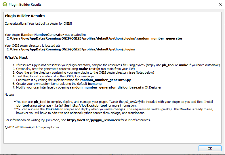
If we now open the new folder “random_number_generator” in the QGIS default plugin folder, you will see the following file structure:
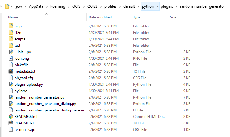
In this introduction to QGIS plugin development, we won’t go into the details of features like internationalization and test code generation, so you can ignore the different subfolders and also some of the files in the main folder. The important files are:
- random_number_generator.py: this file defines the main class RandomNumberGenerator for our plugin. If you look at the code that Plugin Builder 3 generated for this class, you will see that this class has to define a number of methods to interact with QGIS and its plugin interface. One central method is the method run() that in this case here shows our dialog box stored in instance variable self.dlg. If we wanted some code to be executed only if the dialog box is accepted (e.g. closed with the Ok button), then we would put that code here after the “if result:” line.
- random_number_generator_dialog.py: this is the class that defines the main GUI widget for our plugin derived from QDialog. We will talk about this class in more detail in a moment because this is the class that we are going to modify to implement what needs to happen when the user interacts with the GUI of our plugin.
- random_number_generator_dialog_base.ui: this is the class in which the GUI for our dialog box is defined. We will modify it in QT Designer in a moment to adapt the GUI for our purposes.
- __init__.py: A file with this name needs to be contained in the main folder of each plugin and it lets QGIS know about the plugin. QGIS calls the classFactory(…) function defined in this file to create an object of the main class of the plugin (class RandomNumberGenerator in this case).
- metadata.txt: this file contains most of the info about our plugin that we entered into Plugin Builder.
When you now restart QGIS and open the plugin manager under Plugins -> Manage and Install Plugins… , the Random Number Generator plugin should appear in the list of installed plugins but it still needs to be activated. However, if we try to activate it now, we will get an error message that no module called “randomnumbergenerator.resources” can be found. This is a file that we have to generate ourselves by compiling the file called resources.qrc located in our plugin folder with the pyrcc5 tool. The resources file contains information about all additional GUI related resources needed for our plugin, like additional icons for example.
Usually, you would edit the .qrc file first, e.g. in QT Designer, and then compile it. But we don’t need any additional resources for this project, so we just compile it directly with the following command in the OSGeo4W shell after first moving to our plugin folder with the cd command. (The screenshot below contains some commands that were needed in earlier versions of OSGeo4W; you will most likely only need the cd and pyrcc5 commands shown at the bottom.)
pyrcc5 resources.qrc –o resources.py
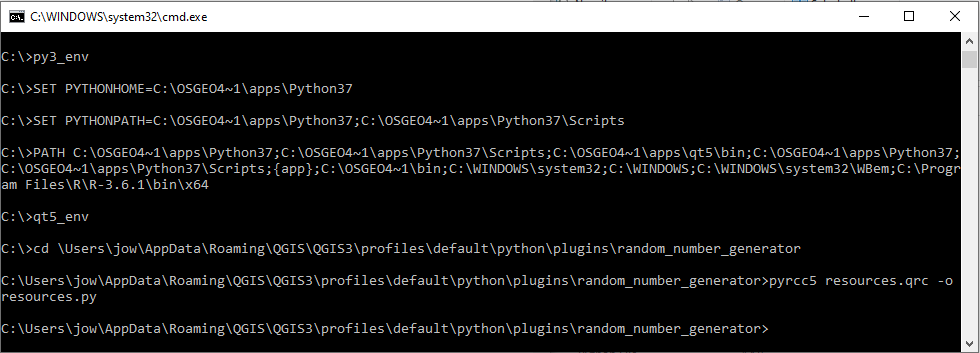
After running this command, we can now activate the plugin by clicking on the checkbox:
There will now be a submenu called “Random Number Generator” with an entry with the same name in the Plugins menu:
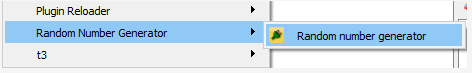
In addition, a toolbar with a single button has been added for our plugin to the toolbar section at the top. Since we didn’t make any changes, the default button  is used. Either clicking the menu entry or the button will open the dialog box for our plugin:
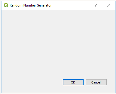
Currently, the dialog box only contains the default elements, namely two buttons for accepting and rejecting the dialog. We are now going to change the GUI of the dialog box and add the random number generation functionality.
4.11.2 Modifying the Plugin GUI and Adding Functionality
The file random_number_generator_dialog.py defines the class RandomNumberGeneratorDialog derived from QDialog. This is the widget class for our dialog box. The GUI itself is defined in the .ui file random_number_generator_dialog_base.ui. In contrast to first compiling the .ui file into a Python .py file and then using the Python code resulting from this to set up the GUI, this class uses the previously briefly mentioned approach of directly reading in the .ui file. That means to change the GUI, all we have to do is modify the .ui file in QT Designer, no compilation needed.
We open random_number_generator_dialog_base.ui with QT Designer and make the following small changes:
- We delete the button box with the Ok and cancel buttons.
- The layout of the dialog box is changed to a vertical layout.
- We add a push button and a label to the dialog box with vertical spacers in between.
- The button text is set to “Press here to generate random number between 1 and 100”.
- The label text is set to “The number is:” and its horizontal alignment property is changed to be horizontally centered.
The image below shows the produced layout in QT Designer.
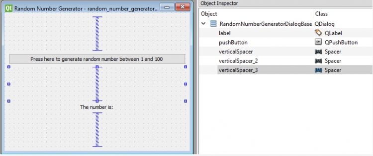
After saving the form, we want to see if we now get the new version of the GUI in QGIS as well. However, for this to happen, the plugin needs to be reloaded. For this, we use the Plugin Reloader plugin that we also installed at the beginning of the lesson. We pick the Plugins -> Plugin Reloader -> Configure option. Then we pick our random_number_generator plugin from the list and press OK.
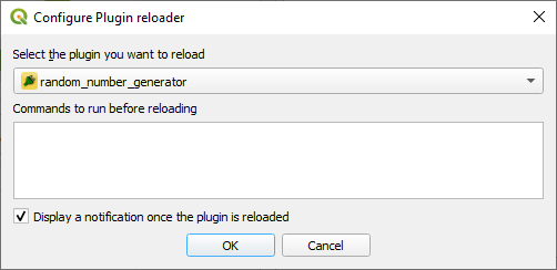
Now we just have to go Plugins -> Plugin Reloader -> Reload: random_number_generator, whenever we want to reload the plugin after making some changes. After doing so and starting our plugin again, it should show up like this in QGIS:
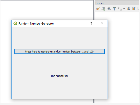
Now we just have to implement the functionality for our plugin, which for this toy example is extremely simple. We just need to write some code for rolling a random number between 1 and 100 and updating the text of the label accordingly when the button is pressed. We implement this in the definition of our class RandomNumberGeneratorDialog in file random_number_generator_dialog.py. The changes we make are the following:
- In the line where the os module is imported, we also import the random module from the Python standard library.
- We add a new method to the class definition with the event handler code:
def generateNewNumber(self): r = random.randint(1,100) self.label.setText("The number is: " + str(r)) - Finally, we connect the button to this new method by adding the following line at the end of the __init__() method:
self.pushButton.clicked.connect(self.generateNewNumber)
Below is the entire code part of random_number_generator_dialog.py after making these changes:
import os, random

from PyQt5 import uic
from PyQt5 import QtWidgets

FORM_CLASS, _ = uic.loadUiType(os.path.join( os.path.dirname(__file__), 'random_number_generator_dialog_base.ui'))

class RandomNumberGeneratorDialog(QtWidgets.QDialog, FORM_CLASS):
    def __init__(self, parent=None):
        """Constructor."""
        super(RandomNumberGeneratorDialog, self).__init__(parent)
        # Set up the user interface from Designer.
        # After setupUI you can access any designer object by doing
        # self.<objectname>, and you can use autoconnect slots - see
        # http://qt-project.org/doc/qt-4.8/designer-using-a-ui-file.html
        # #widgets-and-dialogs-with-auto-connect
        self.setupUi(self)

        self.pushButton.clicked.connect(self.generateNewNumber)

    def generateNewNumber(self):
        r = random.randint(1,100)
        self.label.setText("The number is: " + str(r))
Now the only thing we have to do is reload the plugin again in QGIS, and when we then start the plugin one more time, the button should work and allow us to create random numbers. Please note that the dialog box is opened non-modally from our main plugin class so that you can keep the dialog box open in the background while still interacting with the rest of the QGIS GUI.
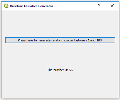
In this small example, all code changes needed were about wiring up the GUI of the dialog box. In such cases, modifying the file with the class definition for the main widget can be sufficient. In the next section, we will implement a plugin that is significantly more complex and interacts with QGIS in more sophisticated ways, e.g., by adding new layers to the currently open project and continuously updating the content of these layers. However, the general approach is the same in that we are mainly going to modify the .ui file and the file with the main widget class from the template files created by Plugin Builder 3. If you want to learn more about QGIS plugin development and the role the other files play, the official documentation [44] is a good starting point.
4.12 Optional: Turning the Bus Event Analyzer into a QGIS Plugin
As said at the beginning of Section 4.11, this section about turning the Bus Track Analyzer code into a plugin that adds new layers to the current QGIS project and displays the analysis progress live on the map canvas can be considered optional. Feel free to just briefly skim through it and then watch the video from Section 4.12.7 showing the final Bus Track Analyzer for QGIS plugin. While creating a QGIS plugin yourself is one option that would give you full over&above points in this lesson's homework assignment, the content of these two sections is not required for the assignment and the quiz. You can always come back to this section if you have time left at the end of this lesson or after the end of the class.
Now that you know how to create plugins for QGIS, let us apply this new knowledge to create a QGIS plugin version of our bus event analyzer from Section 4.10. We will call this plugin “Bus Track Analyzer for QGIS”. The process for this will be roughly as follows:
- Set up a new plugin with Plugin Builder using the Tool “button with dock widget” template
- Copy all the needed files from the project into the plugin folder
- Adapt the default GUI for the dock widget with QT Designer
- Make some smaller modifications to the project files including changes to class BusTrackAnalyzer to define QT signals that we can connect to
- Adapt the code in the dock widget class definition to wire up the GUI and to implement a modified version of the functionality we had in the main program in main.py of the Bus Track Analyzer project
- Implement and integrate a new class QGISEventAndTrackLayerCreator that will be responsible for showing the bus tracks and events detected so far in the QGIS main map window during the analysis
4.12.1 Create Template with Plugin Builder
To create a folder with a template version for this plugin, please follow the steps below.
- Run the Plugin Builder plugin and fill out the first page as follows before clicking “Next >”:
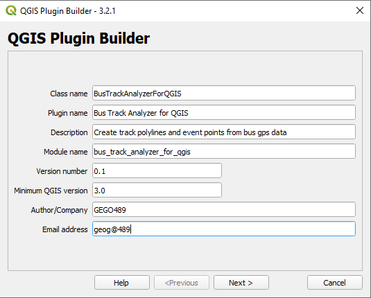 Figure 4.40 First Plugin Builder dialog page with information about the new plugin
 - Just click “Next >” again as we will skip the description part and then on the next page pick the “Tool button with dock widget” template at the top and fill out the rest of the information as shown below before pressing “Next >” again.
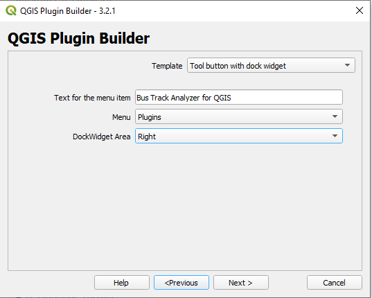 Figure 4.41 Picking the "Tool button with dock widget" template in Plugin Builder
 - We will keep the default settings for the following setup pages, so just keep pressing “Next >” until you arrive at the last page where the button is called “Generate” instead. Take a look at the paths where Plugin Builder is going to create the folder for the new plugin. It might be a good idea to copy the path to somewhere from which you can retrieve it at any time. Now click on “Generate” and the folder for the plugin will be created.
- If you now navigate to the plugins folder from the previous step, it will contain a new folder called “bus_track_analyzer_for_qgis”. Enter that folder and check out the files that have been created. The content should look like this:
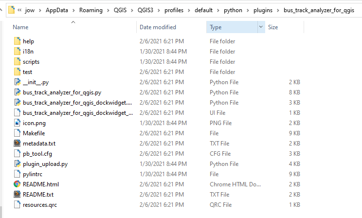 Figure 4.42 Newly created plugin folder with files for our plugin
 - Please close QGIS for a moment. We still need to compile the file resources.qrc into a Python .py file with the help of pyrcc5 as we did in Section 4.11. For this, run OSGeo4W.bat from your OSGeo4W/QGIS installation and, in the shell that opens up, navigate to the folder containing your plugin, e.g. type in the following command but adapt the path to match the path from steps 3 and 4:
cd C:\Users\xyz\AppData\roaming\QGIS\QGIS3\profiles\default\python\plugins\bus_track_analyzer_for_qgis
- Finally, compile the file with the command below. There should now be a file called resources.py in your plugin folder.
pyrcc5 resources.qrc –o resources.py
- You can now restart QGIS and open the plugin manager where “Bus Track Analyzer for QGIS” should now appear in the list of installed plugins. Enable it and then check the Plugins menu to make sure there is now an entry “Bus Track Analyzer for QGIS” there. Start the plugin and a rather empty dock widget will appear in the right part of the QGIS window. Try moving this dock widget around. You will see that you can move it to the other areas of the main QGIS window or completely undock it and have it as an independent window on the screen.
4.12.2 Copy Files into Plugin Folder
For the next steps, it’s best if you again close QGIS for a bit. In case you made any changes to the files during the bus tracking project in Section 4.10, it would be best if you re-download them from here [42]. Then copy the following files from the Section 4.10 project folder (if you didn't edit anything) or the fresh download into the folder for the Bus Tracker plugin:
bus_events.py
bus_track_analyzer.py
bus_tracker_widget.py
core_classes.py
dublin_bus_data.csv
dublin_depots.csv
status_driving.png
status_indepot.png
status_stopped.png
Please note that we are intentionally not including main.py. Also, it wouldn’t really be necessary to include the input data sets (csv files), but there is also no harm in doing so, and it means that we have everything needed to create and run the plugin together in the same folder.
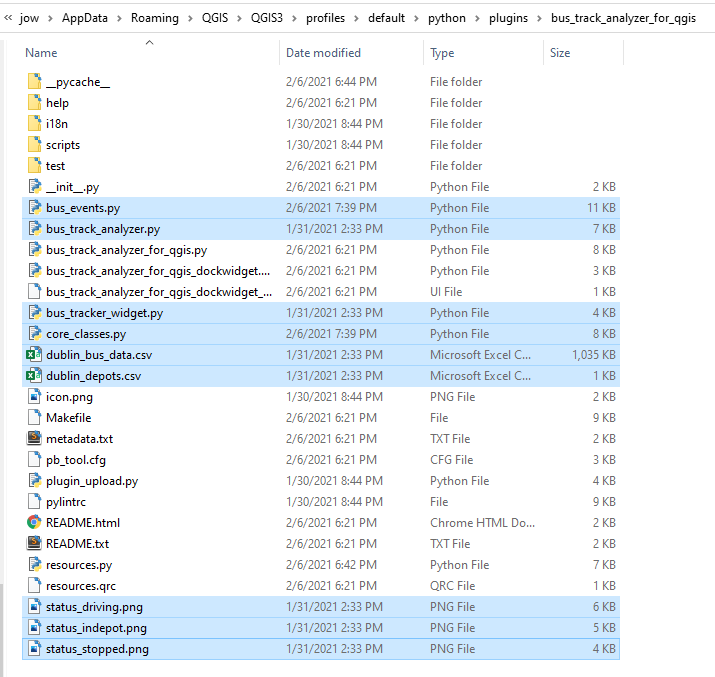
4.12.3 Adapt the GUI with QT Designer
The GUI we will be using for our dock widget is shown in the image below. It has an area at the top where the user can select the GPS and depot input files and a button “Read and init” for reading in the data from the selected files. The central area contains a QScrollArea widget that will host our BusTrackerWidget in the same way as we had it embedded into the main window in the original project. In the area at the bottom, we have the controls for running the analysis consisting of three buttons “Stop and reset”, “Pause”, and “Start” and a QSlider widget for setting the delay between consecutive analysis steps. The image also shows the object names of the important GUI elements that will become instance variables of class BusTrackAnalyzerForQGISDockWidget that we can access and connect to.
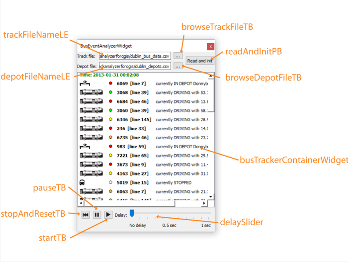
If you look at the files in the folder for our plugin, you will see that Plugin Builder has created a file called bus_track_analyzer_for_qgis_dockwidget.py. This file contains the definition of class BusTrackAnalyzerForQGISDockWidget derived from QDockWidget with the GUI for our plugin. The class itself directly reads the GUI specification from the file bus_track_analyzer_for_qgis_dockwidget_base.ui as explained in Section 4.11.
So the next thing we are going to do is open that .ui file in QT Designer and modify it so that we get the GUI shown in the previous image. The image below shows the new GUI and its widget hierarchy in QT Designer. You don’t have to create this yourself. It is okay if you download the resulting .ui file [45] and extract it into the plugin folder overwriting the default file that is already there (you might need to rename the downloaded file to match the default file). Then open the .ui file in QT Designer for a moment and have a closer look at how the different widgets have been arranged.
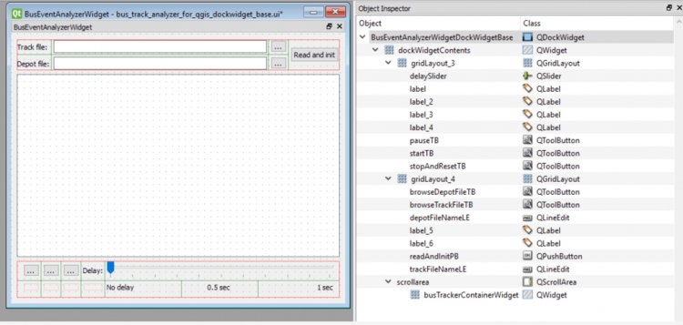
4.12.4 Modifications to the Original Project Files
The next thing we are going to do is make a few smaller changes to the files we copied over from the original project. First of all, it is unfortunately required that we adapt all import statements in which we are importing .py files located in the project folder. The reason is that when we write something like
from core_classes import BusTracker
, this will work fine when the file core_classes.py is located in the current working directory when the program is executed. This is usually the same folder in which the main Python script is located. Therefore, we didn’t have any problems when executing main.py since main.py and the other .py files we wrote are all in the same directory. However, when being run as a QGIS plugin, the working directory will not be the folder containing the plugin code. As a result, you will get error messages when trying to import the other .py files like this. What we have to do is adapt the import statements to start with a dot which tells Python to look for the file in the same folder in which the file in which the import statement appears is located. So the previous example needs to become:
from .core_classes import BusTracker
Here is quick overview of where we have to make these changes:
- In bus_events.py change the import statement at the beginning to:
from .core_classes import Depot, BusTracker
- In bus_track_analyzer.py change the two import statement at the beginning to:
from .bus_events import BusEvent
from .core_classes import BusTracker, Observation, Depot
- Lastly, in bus_tracker_widget.py change the import statement at the beginning to:
from .core_classes import BusTracker
In addition to adapting the import statement, we are going to slightly adapt the bus_track_analyzer.py code to better work in concert with the GUI related classes of our plugin code: we are going to add the functionality to emit signals that we can connect to using the QT signal-slot approach. The two signals we are going to add are the following:
- observationProcessed: This signal will be emitted at the end of the nextStep() method, so whenever the BusTrackAnalyzer object is done with processing one observation, the observation object that has just been processed will be included with the signal.
- eventDetected: This signal will be emitted for each new event that is added to the allEvents list. The emitted signal includes the new bus event object.
Both signals will be used to connect an object of a new class we are going to write in Section 4.12.6 that has the purpose of showing the developing bus tracks and detected events live in QGIS. For this, it is required that the object be informed about newly processed observations and newly detected events, and this is what we are going to facilitate with these signals. Luckily, adding these signals to bus_track_analyzer.py just requires you to make a few small changes:
- Add the following PyQt5 import statement somewhere before the line that starts the class definition with “class BusTrackAnalyzer …”:
from PyQt5.QtCore import QObject, pyqtSignal
- To be able to emit signals we need the class BusTrackerAnalyzer to be derived from the QT class QObject we are importing with the newly added import statement. Therefore, please change the first line of the class definition to:
class BusTrackAnalyzer(QObject):
- Then directly before the start of the constructor with “def __init__...", add the following two lines indented relative to the “class BusTrackAnalyzer…” but not part of any method:
observationProcessed = pyqtSignal(Observation)
eventDetected = pyqtSignal(BusEvent)
With these two lines we are defining the two signals that can be emitted by this class and the types of the parameters they will include.
- Since we are now deriving BusTrackAnalyzer from QObject, we should call the constructor of the base class QObject from the first line of our __init__(…) method. So please add the following line there:
super(BusTrackAnalyzer, self).__init__()
- The last two changes we need to make are both in the definition of the nextStep() method. We therefore show the entire new version of that method here:
  def nextStep(self):
         """performs next step by processing Observation at the front of the Observations priority queue"""
         observation = heapq.heappop(self._observationQueue)           # get Observation that is at front of queue

         # go through list of BusEvent subclasses and invoke their detect() method; then collect the events produced
         # and add them to the allEvents lists
         for evClass in self._eventClasses:
             eventsProduced = evClass.detect(observation, self._depotData, self.allBusTrackers) # invoke event detection method
             self.allEvents.extend(eventsProduced)  # add resulting events to event list
             for event in eventsProduced:
                 self.eventDetected.emit(event)

         # update BusTracker of Observation that was just processed
         observation.busTracker.lastProcessedIndex += 1
         observation.busTracker.updateSpeed()

         if observation.busTracker.status == BusTracker.STATUS_STOPPED: # if  duration of a stopped event has just expired, change status to "DRIVING"
             if observation.timepoint.time > observation.busTracker.statusEvent.timepoint.time + observation.busTracker.statusEvent.duration:
		        observation.busTracker.status = BusTracker.STATUS_DRIVING
                observation.busTracker.statusEvent = None

         # if this was not the last GPS Timepoint of this bus, create new Observation for the next point and add it to the Observation queue
         if observation.timepointIndex < len(observation.busTracker.bus.timepoints) - 1:  # not last point
             heapq.heappush(self._observationQueue, Observation(observation.busTracker, observation.timepointIndex + 1)  )

         # update analyzer status
         self.lastProcessedTimepoint = observation.timepoint

         self.observationProcessed.emit(observation)
In lines 10 and 11 of this new version we added a for-loop that goes through the events produced by the previous call of detect(…) and emit an eventDetected signal for each using the bus event object as a parameter. In the last line of the method, we do the same with the observationProcessed signal including the just processed Observation object.
4.12.5 Implement Main Functionality in BusTrackAnalyzerForQGISDockWidget class
At this point, our plugin is still missing the code that ties everything together, that is, the code that reads in the data from the input files when the “Read and init” button is clicked and reacts to the control buttons at the bottom of the BusTrackAnalyzerForQGISDockWidget widget by starting to continuously call the analyzer’s nextStep() method, pausing that process, or completely resetting the analysis to start from the beginning. We are going to place the code for this directly in the definition of class BusTrackAnalyzerForQGISDockWidget in bus_track_analyzer_for_qgis_dockwidget.py, so you should open that file for editing now. Here is the code that needs to be added, together with some explanations.
- First, we need to important quite a few classes from our own .py files and also a few additional PyQt5 classes; so please change the import statements at the beginning of the code to the following:
import os

from PyQt5 import QtGui, QtWidgets, uic
from PyQt5.QtCore import pyqtSignal, QTimer, QCoreApplication

# added imports
from .bus_track_analyzer import BusTrackAnalyzer
from .bus_tracker_widget import BusTrackerWidget
#from .qgis_event_and_track_layer_creator import QGISEventAndTrackLayerCreator
from .core_classes import Bus, Depot
from .bus_events import LeavingDepotEvent, EnteringDepotEvent, BusStoppedEvent, BusEncounterEvent
Note that we again have to use the notation with the dot at the beginning of the module names here. Also, please note that there is one import statement that is still commented out because it is for a class that we have not yet written. That will happen a bit later in Section 4.12.6 and we will then uncomment this line.
-
Next, we are going to add some initialization code to the constructor, directly after the last line of the __init__(…) method saying “self.setupUi(self)”:
         # own code added to template file

         self.running = False # True if currently running analysis
         self.delay = 0       # delay between steps in milliseconds

         self.eventClasses = [ LeavingDepotEvent, EnteringDepotEvent, BusStoppedEvent, BusEncounterEvent ] # list of event classes to detect
         self.busFileColumnIndices = { 'lon': 8, 'lat': 9, 'busId': 5, 'time': 0, 'line': 1 } # dictionary of column indices for required info

         # create initial BusTrackAnalyzer and BusTrackerWidget objects, and add the later to the scroll area of this widget
         self.analyzer = BusTrackAnalyzer({}, [], self.eventClasses)
         self.trackerWidget = BusTrackerWidget(self.analyzer)
         self.busTrackerContainerWidget.layout().addWidget(self.trackerWidget,0,0)
         self.layerCreator = None    # QGISEventAndTrackLayerCreator object, will only be initialized when input files are read

         # create a QTimer user to wait some time between steps
         self.timer = QTimer()
         self.timer.setSingleShot(True)
         self.timer.timeout.connect(self.step)

         # set icons for play control buttons
         self.startTB.setIcon(QCoreApplication.instance().style().standardIcon(QtWidgets.QStyle.SP_MediaPlay))
         self.pauseTB.setIcon(QCoreApplication.instance().style().standardIcon(QtWidgets.QStyle.SP_MediaPause))
         self.stopAndResetTB.setIcon(QCoreApplication.instance().style().standardIcon(QtWidgets.QStyle.SP_MediaSkipBackward))

         # connect play control buttons and slide to respetive methods defined below
         self.startTB.clicked.connect(self.start)
         self.pauseTB.clicked.connect(self.stop)
         self.stopAndResetTB.clicked.connect(self.reset)
         self.delaySlider.valueChanged.connect(self.setDelay)

         # connect edit fields and buttons for selecting input files to respetive methods defined below
         self.browseTrackFileTB.clicked.connect(self.selectTrackFile)
         self.browseDepotFileTB.clicked.connect(self.selectDepotFile)
         self.readAndInitPB.clicked.connect(self.readData)
What happens in this piece of code is the following:
- First, we introduce some new instance variables for this class that are needed for reading data and setting up a BusTrackAnalyzer object (you probably recognize the variables eventClasses and busFileColumnIndices from the original main.py file) and for controlling the analysis steps. Variable running will be set to True when the analyzer’s nextStep() method is supposed to be called continuously with small delays between the steps whose length is given by variable delay. It is certainly not optimal that the column indices for the GPS data file are hard-coded here in variable busFileColumnIndices but we decided against including an option for the user to specify these in this version to keep the GUI and code as simple as possible.
- In the next block of code, we create an instance variable to store the BusTrackAnalyzer object we will be using, and we create the BusTrackerWidget widget and place it within the scroll area in the center of the GUI. Since we have not read any input data yet, we are using an empty bus dictionary and empty depot list to set these things up.
- An instance variable for a QTimer object is created that will be used to queue up the execution of the method step() defined later when the widget is in continuous execution mode.
- The next code block simply sets the icons for the different control buttons at the bottom of the widget using standard QT icons.
- Next, we connect the “clicked” signals of the different control buttons to different methods of the class that are supposed to react to these signals. We do the same for the “valueChanged” signal of the QSlider widget in our GUI to be able to adapt the value of the variable delay when the slider is moved by the user.
- Finally, we link the three buttons at the top of the GUI for reading in the data to the respective event handler methods.
-
Now the last thing that needs to happen is adding the different event handler methods we have already been referring to in the previously added code. This is another larger chunk of code since there are quite a few methods to define. Please add the definitions at the end of the file after the definition of the method closeEvent(…) that is already there by default.
     # own methods added to template file

     def selectTrackFile(self):
         """displays open file dialog to select bus track input file"""
         fileName, _ = QtWidgets.QFileDialog.getOpenFileName(self,"Select CSV file with bus track data", "","(*.*)")
         if fileName:
             self.trackFileNameLE.setText(fileName)

     def selectDepotFile(self):
         """displays open file dialog to select depot input file"""
         fileName, _ = QtWidgets.QFileDialog.getOpenFileName(self,"Select CSV file with depot data", "","(*.*)")
         if fileName:
             self.depotFileNameLE.setText(fileName)

     def readData(self):
         """reads bus track and depot data from selected files and creates new analyzer and creates analyzer and layer creator for new input"""
         if self.running:
             self.stop()
         try:   # read data
             depotData = Depot.readFromCSV(self.depotFileNameLE.text())
             busData = Bus.readFromCSV(self.trackFileNameLE.text(), self.busFileColumnIndices)
         except Exception as e:
             QtWidgets.QMessageBox.information(self, 'Operation failed', 'Could not read data from files provided: '+ str(e.__class__) + ': ' + str(e), QtWidgets.QMessageBox.Ok)
             busData = {}
             depotData = []

         # create new analyzer and layer creator objects and connect them
         self.analyzer = BusTrackAnalyzer(busData, depotData, self.eventClasses)
         self.trackerWidget.analyzer = self.analyzer
#         self.createLayerCreator()
         self.trackerWidget.updateContent()

     def stop(self):
         """halts analysis but analysis can be continued from this point"""
         self.timer.stop()
         self.running = False

     def reset(self):
         """halts analysis and resets analyzer to start from the beginning"""
         self.stop()
         self.analyzer.reset()
#         self.createLayerCreator()
         self.trackerWidget.updateContent()

     def start(self):
         """starts analysis if analysis isn't already running"""
         if not self.running:
             self.running = True
             self.step()

     def step(self):
         """performs a single analysis step of the BusTrackAnalyzer but starts singleshot timer after each step to call itself again"""
         if self.running:
             if self.analyzer.isFinished():
                 self.stop()
             else:
                 self.analyzer.nextStep()               # perform next analysis step
                 self.trackerWidget.updateContent()     # redraw tracker widget
                 self.timer.start(max([5,self.delay])) # start timer to call this method again after delay

     def setDelay(self):
         """adapt delay when slider has been moved"""
         self.delay = 10 * self.delaySlider.value()
         if self.running:                           # if analysis is running, change to the new delay immediately
             self.timer.stop()
             self.timer.start(max([5,self.delay]))
The first two methods selectTrackFile() and selectDepotFile() are called when the “…” buttons at the top are clicked and will open file dialog boxes for picking the input files. The method readData() is invoked when the “Read and init” button is clicked. It stops all ongoing executions of the analyzer, attempts to read the data from the selected files, and then creates a new BusTrackAnalyzer object for this input data and connects it to the BusTrackerWidget in our GUI. The code of this function contains another two lines that are commented out and that we will uncomment later.
The other methods we define in this piece of code are the event handler functions for the control buttons at the bottom:
- stop() is called when the “Pause” button in the middle is clicked and simply stops the timer if its currently running and sets the variable running to False so that the analyzer’s nextStep() method won’t be called anymore.
- reset() is called when the control button on the left is called and it also stops the execution but, in addition, resets the analyzer so that the analysis will start from the beginning when the “Start” button is clicked again.
- start() is called when the right control button (“Play”) for continuously performing analysis steps is clicked. It sets variable running to True and then invokes method step() to run the first analysis step.
- step() is either called from start() or by the timer it sets up itself after each call of the analyzer’s nextStep() method to perform the next analysis step after a certain delay until all observations have been processed. Please note that we are using minimum delay of 5 milliseconds to make sure that the QGIS GUI remains responsive while we are running the analysis.
- setDelay() is called when the slider is moved and it translates the slider position into a delay value between 0 and 1 second. It also immediately restarts the timer to use this new delay value.
Our plugin is operational now and you can open QGIS and run it. In case you already have QGIS running or you encounter any errors that need to be fixed, don’t forget to reload the plugin code with the help of the Plugin Reloader plugin. Once the dock widget appears at the right side of the QGIS window (as shown in the figure below), do the following:
- Use the “…” buttons to select the input files for the bus GPS and depot data.
- Click “Read and init”; after that you should see the initial bus tracker configuration in the central area of the dock widget.
- Press the “Play” button to start the analysis; the content of the BusTrackerWidget should now continuously update to reflect the current state of the analysis
- Test out the “Pause” and “Rewind” buttons as well as changing the delay between steps with the slider to control the speed the analysis is run at.
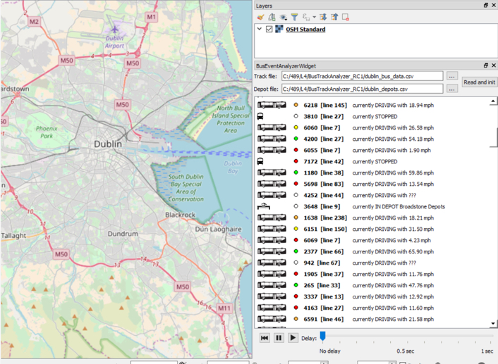
So far, so good. We have now turned our original standalone project into a QGIS plugin and even added in some extra functionality allowing the user to pause and restart the analysis and control the speed. However, typically a QGIS plugin in some way interacts with the content of the project that is currently open in QGIS, for instance by taking some of its layers as input or adding new layers to the project. We will add this kind of functionality in the next section and this will be the final addition we are making to our plugin.
4.12.6 Create and Integrate New Class QGISEventAndTrackLayerCreator
In addition to showing the current bus tracker states in the dock widget, we want our plugin to add two new layers to the currently open QGIS project that show the progress of the analysis and, once the analysis is finished, contain its results. The two layers will correspond to the two output files we produced in the original project in Section 4.10:
- a polyline layer showing routes taken by the different bus vehicles with the bus IDs as attribute,
- a point layer showing the detected events with the type of the event and a short description as attributes.
Since we don’t want to just produce these layers at the end of the analysis but want these to be there from the start of the analysis and continuously update whenever a new bus GPS observation is processed or an event is detected, we are going to write some code that reacts to the observationProcessed and eventDetected signals emitted by our class BusTrackAnalyzer (see the part of Section 4.12.4 where we added these signals). We will define a new class for all this that will be called QGISEventAndTrackLayerCreator and it will be defined in a new file qgis_event_and_track_layer_creator.py. The class definition consists of the constructor and two methods called addObservationToTrack(…) and addEvent(…) that will be connected to the corresponding signals of the analyzer.
Let’s start with the beginning of the class definition and the constructor. All following code needs to be placed in file qgis_event_and_track_layer_creator.py that you need to create in the plugin folder.
import qgis

class QGISEventAndTrackLayerCreator():

     def __init__(self):
         self._features = {}    # dictionary mapping bus id string to polyline feature in bus track layer
         self._pointLists = {}  # dictionary mapping bus id string to list of QgsPointXY objects for creating the poylines from

         # get project currently open in QGIS
         currentProject = qgis.core.QgsProject.instance()

         # create track layer and symbology, then add to current project
         self.trackLayer = qgis.core.QgsVectorLayer('LineString?crs=EPSG:4326&field=BUS_ID:integer', 'Bus tracks' , 'memory')
         self.trackProv = self.trackLayer.dataProvider()

         lineMeta = qgis.core.QgsApplication.symbolLayerRegistry().symbolLayerMetadata("SimpleLine")
         lineLayer = lineMeta.createSymbolLayer({'color': '0,0,0'})
         markerMeta = qgis.core.QgsApplication.symbolLayerRegistry().symbolLayerMetadata("MarkerLine")

         markerLayer = markerMeta.createSymbolLayer({'width': '0.26', 'color': '0,0,0', 'placement': 'lastvertex'})
         symbol = qgis.core.QgsSymbol.defaultSymbol(self.trackLayer.geometryType())
         symbol.deleteSymbolLayer(0)
         symbol.appendSymbolLayer(lineLayer)
         symbol.appendSymbolLayer(markerLayer)

         trackRenderer = qgis.core.QgsSingleSymbolRenderer(symbol)
         self.trackLayer.setRenderer(trackRenderer)

         currentProject.addMapLayer(self.trackLayer)

         # create event layer and symbology, then add to current project
         self.eventLayer = qgis.core.QgsVectorLayer('Point?crs=EPSG:4326&field=TYPE:string(50)&field=INFO:string(255)', 'Bus events' , 'memory')
         self.eventProv = self.eventLayer.dataProvider()

         colors = { "BusEncounterEvent": 'yellow', "BusStoppedEvent": 'orange', "EnteringDepotEvent": 'blue', "LeavingDepotEvent": 'green' }

         categories = []
         for ev in colors:
             categories.append( qgis.core.QgsRendererCategory( ev, qgis.core.QgsMarkerSymbol.createSimple({'name': 'square', 'size': '3.0', 'color': colors[ev]}), ev ))

         eventRenderer = qgis.core.QgsCategorizedSymbolRenderer("TYPE", categories)
         self.eventLayer.setRenderer(eventRenderer)

         currentProject.addMapLayer(self.eventLayer)
To be able to build polylines for the bus tracks and update these whenever a new observation has been processed by the analyzer, we need to maintain dictionaries with the QGIS features and point lists for each bus vehicle track. These are created at the beginning of the constructor code in lines 6 and 7. In addition, the constructor accesses the currently open QGIS project (line 10) and adds the two new layers called “Bus tracks” and “Bus events” to it (lines 29 and 44). The rest of the code is mainly for setting the symbology of these two layers: For the track layer, we use black lines with a red circle marker at the end to indicate the current location of the vehicle (lines 16 to 27) as shown in the image below. For the events, we use square markers in different colors based on the TYPE of the event (lines 35 to 42).
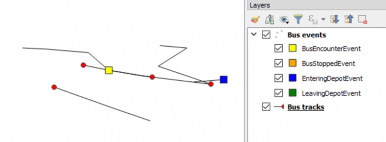
Now we are going to add the definition of the method addObservationToTrack(…) that will be connected to the observationProcessed signal emitted when the analyzer object has completed the execution of nextStep().
	def addObservationToTrack(self, observation):
         """add new vertex to a bus polyline based on the given Observation object"""
         busId = observation.busTracker.bus.busId;

         # create new point for this observation
         p =  qgis.core.QgsPointXY(observation.timepoint.lon, observation.timepoint.lat)

         # add point to point list and (re)create polyline geometry
         if busId in self._features:      # we already have a point list and polyline feature for this bus
             feat = self._features[busId]
             points = self._pointLists[busId]
             points.append(p)

             # recreate polyline geometry and replace in layer
             polyline = qgis.core.QgsGeometry.fromPolylineXY(points)
             self.trackProv.changeGeometryValues({feat.id(): polyline})

         else:                            # new bus id we haven't seen before
             # create new  polyline and feature
             polyline = qgis.core.QgsGeometry.fromPolylineXY([p])
             feat = qgis.core.QgsFeature()
             feat.setGeometry(polyline)
             feat.setAttributes([int(busId)])
             _, f = self.trackProv.addFeatures([feat])
             # store point list and polyline feature in respective dictionaries
             self._features[busId] = f[0]
             self._pointLists[busId] = [p]

         # force redraw of layer
         self.trackLayer.triggerRepaint()
         qgis.utils.iface.mapCanvas().refresh()
The Observation object given to this method as a parameter provides us with access to all the relevant information we need to update the polyline feature for the bus this observation is about. First, we extract the ID of the bus (line 3) and create a new QgsPointXY object from the Timepoint stored in the Observation object (line 6). If we already have a polyline feature for this vehicle, we get the corresponding feature and point lists from the features and pointLists dictionaries, add the new point to the point list and create a new polyline geometry from it, and finally change the geometry of that feature in the bus track layer to this new geometry (lines 10 to 16). If instead this is the first observation of this vehicle, we create a point list for it to be stored in the pointList dictionary as well as a new polyline geometry with just that single point, and we then set up a new QgsFeature object for this polyline that is added to the bus track layer and also the features dictionary (lines 19 to 27). At the very end of the method, we make sure that the layer is repainted in the QGIS map canvas.
Now we add the code for the addEvent(…) method completing the definition of our class QGISEventAndTrackLayerCreator:
		def addEvent(self, busEvent):
         	"""add new event point feature to event layer based on the given BusEvent object"""
            # create point feature with information from busEvent
            p =  qgis.core.QgsPointXY(busEvent.timepoint.lon, busEvent.timepoint.lat)
            feat = qgis.core.QgsFeature()
            feat.setGeometry(qgis.core.QgsGeometry.fromPointXY(p))
            feat.setAttributes([type(busEvent).__name__, busEvent.description()])

            # add feature to event layer and force redraw
            self.eventProv.addFeatures([feat])

            self.eventLayer.triggerRepaint()
            qgis.utils.iface.mapCanvas().refresh()
This method is much simpler because we don’t have to modify existing features in the layer but rather always add one new point feature to the event layer. All information required for this is taken from the bus event object given as a parameter: The coordinates for the next point feature are taken from the Timepoint stored in the event object (line 4), for the TYPE field of the event we take the type of the event object (line 7), and for the INFO field we take the string returned by calling the event object’s description(…) method (also line 7).
To incorporate this new class into our current plugin, we need to make a few more modifications to the class BusTrackAnalyzerForQGISDockWidget in file bus_track_analyzer_for_qgis_dock_widget.py. Here are the instructions for this:
- Remove the # at the beginning of the line “from .qgis_event_and_track_layer_creator import …” to uncomment this line and import our new class.
- Now we add a new auxiliary method to the class definition that has the purpose of creating an object of our new class BusTrackAnalyzerForQGISDockWidget and connecting its methods to the corresponding signals of the analyzer object. Add the following definition as the first method after the “closeEvent” method, so directly after the comment “# own methods added to the template file”.
	def createLayerCreator(self):
         """creates a new QGISEventAndTrackLayerCreator for showing events and tracks on main QGIS window and connects it to analyzer"""
         self.layerCreator = QGISEventAndTrackLayerCreator()
         self.analyzer.observationProcessed.connect(self.layerCreator.addObservationToTrack)
         self.analyzer.eventDetected.connect(self.layerCreator.addEvent)
We already set up an instance variable layerCreator in the constructor code and we are using it here for storing the newly created layer creator object. Then we connect the signals to the two methods of the layer creator object.
- Now we just need to uncomment two lines to make sure that the method createLayerCreator() is called at the right places, namely after we read in data from the input files and when the analyzer is reset. In both cases, we want to create a new layer creator object that will set up two new layers in the current QGIS project. The lines that you need to uncomment for this by removing the leading # are:
- the line “# self.createLayerCreator()” in method readData()
- the line “# self.createLayerCreator()” in method reset()
You should make sure that the indentation is correct after removing the hashmarks.
That’s it, we are done with the code for our plugin!
4.12.7 Try It Out
To try out this new version of the plugin, close the dock widget if it’s currently still open in QGIS and then run the Plugin Reloader plugin to load this updated version of our plugin. Add a basemap to your map project and zoom it to the general area of Dublin. When you then load the input files, you will see the two new layers appear in the layer list of the current QGIS project with the symbology we are setting up in the code. When you now start the analysis, what you see should look like the video below with the bus tracker widget continuously updating the bus status information, the bus tracks starting to appear in the QGIS map window, and square symbols starting to pop up for the events detected.
[NOTE: This video (3:04) does NOT contain sound]
The delay slider can be used to increase the breaks between two analysis steps, which can be helpful if the map window doesn’t seem to update properly because QGIS has problems catching up with the requests to repaint layers. This in particular is a good idea if you want to pan and zoom the map in which case you may notice the basemap tiles not appearing if the delay is too short.
Overall, there is quite a bit that could be optimized to make sure that QGIS remains responsive while the plugin and analysis are running as well as other improvements and extensions that could be made. But all this would increase the amount of code needed quite a bit and this has already been a rather long project to begin with, requiring you to read and understand a lot of code. As we said before, it is not required to understand each line in the code; the crucial points to understand are how we are using classes, objects, and inheritance in this project and make use of the other techniques and concepts taught in this lesson. Reading and understanding other people’s code is one of the main ways to become a better programmer and since we are approaching the end of this course, this was a good place to practice this a bit and maybe provide some inspiration for your term project. However, we certainly don’t expect your term project to be nearly as complex as the plugin created in this section!
4.13 Lesson 4 Practice Exercise
The focus in this lesson has been on object-oriented programming in Python and applying it in the context of QGIS to create GUI-based programs and plugins. In the only practice exercise of this lesson, we are going to apply the concepts of self-defined classes, inheritance and overriding methods to build a standalone GIS tool based on the qgis package that is significantly simpler than the project from the lesson walkthroughs. As before, this is intended as a preparation for this lesson's homework assignment in which you are supposed to create a somewhat larger object-oriented tool.
Here is the task: You have been given a .csv file that contains observations of animals in Kruger National Park. Each row in the .csv file contains a unique ID for the observed animal and the latitude and longitude coordinates of the observation, in that order. The observations are ordered chronologically. The test file we will be working with has just the following nine rows. Please download the L4exercise_data.zip file [46] containing this data.
123AD127,-23.965517,31.629621
183AE121,-23.921094,31.688953
223FF097,-23.876783,31.661707
183AE121,-23.876783,31.661707
123AD121,-23.961818,31.694983
223FF097,-24.083749,31.824532
123AD127,-24.083749,31.824532
873TF129,-24.040581,31.426711
123AD127,-24.006232,31.428593
The goal is to write a standalone qgis script that produces a point GeoPackage file with a point feature for just the first observation of each animal occurring in the .csv file. The file contains observations for five different animals and the result when opened in QGIS should look like this:
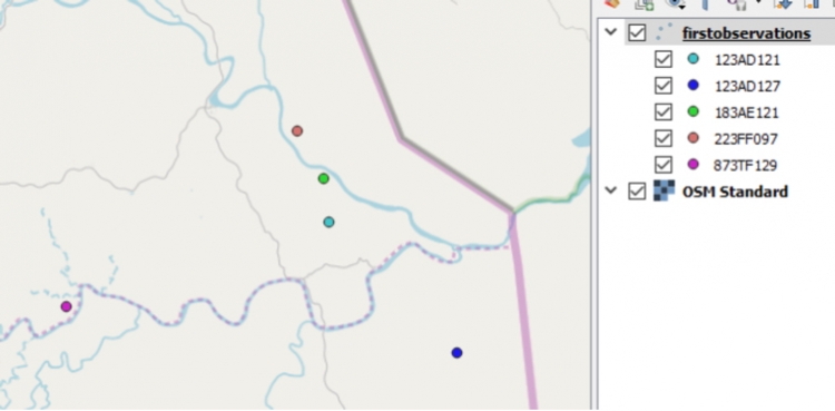
You have already produced some code that reads the data from the file into a pandas data frame stored in variable data. You also want to reuse a class PointObject that you already have for representing point objects with lat and lon coordinates and that has a method called toQgsFeature(…) that is able to produce and return a QgsFeature (see again Section 4.5.3) for a point object of this class.
import qgis
import sys, os
import pandas as pd

# create pandas data frame from input data
data = pd.read_csv(r"C:\489\L4\exercise\L4exercise_data.csv")

class PointObject():

    # constructor for creating PointObject instances with lon/lat instance variables
    def __init__(self, lat, lon):
        self.lon = lon
        self.lat = lat

    # methods for creating QgsFeature object from a PointObject instance
    def toQgsFeature(self):
        feat = qgis.core.QgsFeature()
        feat.setGeometry(qgis.core.QgsGeometry.fromPointXY(qgis.core.QgsPointXY(self.lon, self.lat)))
        return feat

firstObservations = []          # for storing objects of class pointWithID
firstObservationsFeatures = []  # for storing objects of class QgsFeature
When you look at method toQgsFeature(), you will see that it creates a new QgsFeature (see Section 4.5.3), sets the geometry of the feature to a point with the given longitude and latitude coordinates, and then returns the feature. Since PointObject does not have any further attributes, no attributes are defined for the created QgsFeature object.
Your plan now is to write a new class called PointWithID that is derived from the class PointObject and that also stores the unique animal ID in an instance variable. You also want to override the definition of toQgsFeature() in this derived class (see again Section 4.7), so that it also uses setAttributes(…) to make the ID of the animal an attribute of the produced QgsFeature object. To do this, you can first call the toQgsFeature() method of the base class PointObject with the command
super(PointWithID, self).toQgsFeature()
… and then take the QgsFeature object returned from this call and set the ID attribute for it with setAttributes(…).
Furthermore, you want to override the == operator for PointWithID so that two objects of that class are considered equal if their ID instance variable are the same. This will allow you to store the PointWithID objects created in a list firstObservations and check whether or not the list already contains an observation for the animal in a given PointWithID object in variable pointWithID with the expression
pointWithID in firstObservations
To override the == operator, class PointWithID needs to be given its own definition of the __eq__() method as shown in Section 4.6.2.
What you need to do in this exercise is:
- Define the class PointWithID according to the specification above.
- Add the code needed for making this a standalone qgis program (Sections 4.5.4 and 4.10.2.4).
- Implement a loop that goes through the rows of the pandas data frame (with data.itertuples(), Section 3.8.2) and creates an object of the class PointWithID for the given row, then adds this object to list firstObervations, unless the list already contains an object with the same animal ID.
- Add the code for creating the new point layer with EPSG:4326 as the CRS.
- Make firstObservationFeatures a list with a QgsFeature object for each PointWithID object in list firstObservations using the overridden toQgsFeature() method. Then add all features from that new list to the new layer (Section 4.5.3).
- Finally, write the new layer to a new GeoPackage file and check whether or not you get the same result as shown in the image above.
4.13.1 Lesson 4 Practice Exercise Solution and Explanation
Solution
import qgis
import qgis.core
import sys, os
import pandas as pd


# read data into pandas data frame
data = pd.read_csv(r"C:\489\L4\exercise\L4exercise_data.csv")

# class definition for PointObject
class PointObject():

    def __init__(self, lat, lon):
        self.lon = lon
        self.lat = lat

    def toQgsFeature(self):
         feat = qgis.core.QgsFeature()
         feat.setGeometry(qgis.core.QgsGeometry.fromPointXY(qgis.core.QgsPointXY(self.lon, self.lat)))
         return feat

firstObservations = []          # for storing objects of class pointWithID
firstObservationsFeatures = []  # for storing objects of class QgsFeature

# code for creating QgsApplication and initializing QGIS environment
qgis_prefix = os.getenv("QGIS_PREFIX_PATH")
qgis.core.QgsApplication.setPrefixPath(qgis_prefix, True)
qgs = qgis.core.QgsApplication([], False)
qgs.initQgis()

# definition of class PointWithID derived from PointObject
# to represent animal observation from the input data
class PointWithID(PointObject):

    def __init__(self, pID, lat, lon):
        super(PointWithID, self).__init__(lat, lon)
        self.pID = pID  # instance variable for storing animal ID

    # overwriting the == operator to be based on the animal ID
    def __eq__(self, other):
        return self.pID == other.pID

    # overwriting this method to include animal ID as attribute of QgsFeature created
    def toQgsFeature(self):
         feat = super(PointWithID, self).toQgsFeature()
         feat.setAttributes([self.pID])
         return feat

# create list of PointWithID object with first observations for each animal in the data frame
for row in data.itertuples(index=False):
    pointWithID = PointWithID(row[0], row[1], row[2])
    if not pointWithID in firstObservations: # here __eq__() is used to do the comparison
        firstObservations.append(pointWithID)

# list comprehension for creating list of features from firstObservations list
firstObservationsFeatures = [ o.toQgsFeature() for o in firstObservations ]

# create new point layer with field for animal ID
layer = qgis.core.QgsVectorLayer("Point?crs=EPSG:4326&field=AnimalID:string(255)", 'animal first observations' ,'memory')

# add features to new layer
prov = layer.dataProvider()
prov.addFeatures(firstObservationsFeatures)

# save layer as GeoPackage file
qgis.core.QgsVectorFileWriter.writeAsVectorFormat( layer, r"C:\489\L4\exercise\firstobservations.gpkg", "utf-8",layer.crs(), "GPKG")

# clean up
qgs.exitQgis()
Explanation
- In line 34 the new class PointWithID is declared to be derived from class PointObject.
- The constructor in line 36 calls the constructor of the base class and then adds the additional instance variable for the animal ID (called pID).
- __eq__() is defined in lines 43 and 44 to compare the pID instance variables of both involved objects and return True if they are equal.
- In lines 48 and 49, we call toQgsFeature() of the base class PointObject and then take the returned feature and add the animal ID as the only attribute.
- In lines 53 to 56, we use itertuples() of the data frame to loop through its rows. We create a new PointWithID object in variable pointWithID from the cell values of the row and then test whether an object with that ID is already contained in list firstObservations. If not, we add this object to the list.
- In line 59, we use toQgsFeature() to create a QgsFeature object from each PointWithID object in the list. These are then added to the new layer in line 66.
- When creating the new layer in line 62, we have to make sure to include the field for storing the animal ID in the string for the first parameter.
4.14 Lesson 4 Assignment
In this final homework assignment, the task is to create a qgis based program, simpler than the Bus Track Analyzer from the lesson walkthrough but also involving the definition of a class hierarchy and static class functions to identify instances of the classes in the input data. While it is an option to submit a QGIS plugin rather than a standalone tool for over&above points, this is not a requirement and, therefore, it is not needed that you have worked through Section 4.11 and 4.12 in detail. The main code for the tool you are going to implement will include a class hierarchy with classes for different types of waterbodies (streams, rivers, lakes, ponds, etc.) and the tool's purpose will be to create two new vector data sets from a JSON data export from OpenStreetMap (OSM).
The situation is the following: you are working on a hydrology related project. As part of the project you frequently need detailed and up-to-date vector data of the waterbodies in different areas and one source you have been using to obtain this data is OpenStreetMap. To get the data you are using the Overpass API [47] running queries like the following
https://www.overpass-api.de/api/interpreter?data=[out:json];(way["natural"="water"](40.038844,-79.006452,41.497860,-76.291359);way["waterway"]
(40.038844,-79.006452,41.497860,-76.291359););(._;>;);out%20body;
to obtain all OSM “way” elements (more on ways and the OSM data model in a moment) with certain water related tags.
An overpass query like this will return a JSON document listing all the way entities with the required tags and their nodes with coordinates. Nodes are point features with lat / lon coordinates and ways are polyline or polygon features whose geometry is defined via lists of nodes. If you are not familiar with the OSM concepts of nodes, ways, and relations, please take a moment to read “The OpenStreetMap data model." [48]
The only data you will need for this project is the JSON input file [49] we will be using. Download it and extract it to a new folder, then open it in a text editor. You will see that the JSON code in the file starts with some meta information about the file and then has an attribute called “elements” that contains a list of all OSM node elements followed by all OSM way elements (you have to scroll down to the end to see the way elements because there are many more nodes than ways in the query result).
All node definitions in the “elements” list have the following structure:
{
  "type": "node",
  "id": 25446505,
  "lat": 40.2585099,
  "lon": -77.0521733
},
The “type” attribute makes it clear that this JSON element describes an OSM node. The “id” attribute is a unique identifier for the node and the other two attributes are the latitude and longitude coordinates.
All way definitions in the “elements” list have the following structure:
{
  "type": "way",
  "id": 550714146,
  "nodes": [
    5318993708,
    5318993707,
    5318993706,
    ...
    5318993708
  ],
  "tags": {
    "name": "Wilmore Lake",
    "natural": "water",
    "water": "reservoir"
  }
},
The attribute “type” signals that this JSON element describes an OSM way feature. The “id” attribute contains a unique ID for this way and the “nodes” attribute contains a list of node IDs. If the IDs of the first and last nodes in this list are identical (like in this case), this means that this is a closed way describing an areal polygon geometry, rather than a linear polyline geometry. To later create QGIS geometries for the different waterbodies, you will have to take the node list of a way, look up the corresponding nodes based on their IDs, and take their coordinates to create the polygon or polyline feature from.
In addition, the JSON elements for ways typically (but not always!) contain a “tags” attribute that stores the OSM tags for this way. Often (but not always!), ways will have a “name” tag (like in this case) that you will have to use to get the name of the feature. In this example, the way also has the two tags “natural” with the value “water” assigned and “water” with the value “pond” assigned. The way in which waterbodies are tagged in OSM has been criticized occasionally and suggestions for improvements have been made. Right now, waterbodies typically either have been tagged with the key “waterway” [50] with the assigned value being a particular type like “stream” or “river”, or with the combination of the key “natural” being assigned the value “water” and the key “water” being assigned a specialized type like “lake” or “pond”. Luckily, you don’t have to worry too much about the inconsistencies and disadvantages of the OSM tagging for waterbodies because you will below be given concrete rules on how to identify the different types of waterbodies we are interested in.
In lesson 2, we already talked about JSON code and that it can be turned into a nested Python data structure that consists of lists and dictionaries. In lesson 2, we got the JSON from web requests and we therefore used the requests module for working with the JSON code. In the context of this assignment, it makes more sense to use the json module from the standard library to work with the provided JSON file. You can simply load the JSON file and create a Python data structure from the content using the following code assuming that the name and path to the input file are stored in variable filename:
import json

with open(filename, encoding = "utf8") as file:
	data = json.load(file)
After this, you can, for instance, use the expression data["elements"] to get a list with the content that is stored in the top-level “elements” attribute. To get the first element from that list which will be the description of an OSM node, you'd use data["elements"][0] and data["elements"][0]["id"] refers to the ID of that node, while data["elements"][0]["type"]will return the string 'node' providing a way to check what kind of OSM element you are dealing with. The page “How-to-parse-json-string-in-python” [51] contains an example of how to access elements at different levels in the JSON structure that might be helpful here. If you have any questions about handling JSON code while working on this assignment, please ask them on the forums.
In order to later create polyline or polygon geometries from the OSM way elements in the input file, we will have to look up node elements based on the node IDs that we find in the "nodes" lists of the way elements to get to the latitude and longitude coordinates of these nodes. A good first step, therefore, is to create seperate dictionaries for the node and way elements using the IDs as key such that we can use the IDs to get to the entire node or way description as a Python dictionary. The following code creates these dictionaries from the content of variable data:
nodesDict = {}  # create empty dictionary for the node elements
waysDict = {}   # create empty dictionary for the way elements

for element in data['elements']:            # go through all elements in input data
    if element['type'] == 'node':           # check if element is an OSM node
        nodesDict[element['id']] = element  # place element in nodes dictionary using its ID as the key
    elif element['type'] == 'way':          # check if element is an OSM way
        waysDict[element['id']] = element   # place element in ways dictionary using its ID as the key
Now that this is done we can loop through all way elements using the following code:
for wayID in waysDict:       # go through all keys (= way IDs)
    way = waysDict[wayID]    # get the way element for the given ID
    print(way)
    ... # do something else with way, e.g. access its node list with way['nodes']
Since each node or way element is again represented by a Python dictionary, the output we get from the print statement will look as below and we can, for instance, use way['nodes'] or way['tags'] to refer to the different properties of the way element.
{'type': 'way', 'id': 4251261, 'nodes': [25446505, 618262874, 25446506, 618262877, 618262880, 5421855904, 25446508, 4568980789, 4568980790, 4568980791, 4568980792, 618264570, 4568980793, 4568980794, 4568980795, 618264571, 25446510, 4568980796, 4568980797, 618264572, 4568980798, 4568980799, 618264573, 4568980800, 25446511, 618264574, 25446512, 618264575, 25446513, 618264576, 618264577, 25446514, 618264578, 25446516, 5417811540, 618264580, 25446560, 25446517], 'tags': {'name': 'Conodoguinet Creek', 'waterway': 'river'}}
Furthermore, whenever we have a node ID and need to get the information for that node, we can look it up in the nodes dictionary:
nodeID = 5318993708    # some exemplary node ID

node = nodesDict[nodeID]   # get the node element we have stored under that ID
print(node)
Again, keep in mind that a node is represented by a Python dictionary. Hence, the output from the print statement will look as below and we can, for instance, use node['lat'] and node['lon'] to refer to the latitude and longitude coordinates of that node.
{'type': 'node', 'id': 5318993708, 'lat': 40.4087294, 'lon': -78.6877245}
Before you read on, we recommend that you make sure you have a good understanding of what the code above does and how to work with the nested dictionary structures containing the way and node information. Play around with the code a bit. For instance, try to modify the loop that goes through the way elements such that it checks whether or not the given way elements contain a 'tags' property and if so, whether or not the tags dictionary contains an 'name' entry. If so, print out the name stored there. E.g. for the first way element shown above, the produced output should be just Conodoguinet Creek.
Your task
Your task now is to implement a tool based on the qgis Python package with at least a basic GUI that allows the user to select an input .json file on disk. When the user presses a button, the tool reads in all the node and way information from the json file into two dictionaries that allow for accessing the different node and way entities by their ID as we showed above.
Next, the program should loop through all the way entities and create objects of the six different waterbody classes Stream, River, Canal, Lake, Pond, and Reservoir depending on how the ways are tagged. The first three of these classes are for linear features that will be represented by polylines later on. The other three are for areal features that will be represented by polygons. Your tool should produce two new vector data sets in the GeoPackage format, one with all linear features and one with all areal features that look as shown in the image below when added to QGIS.
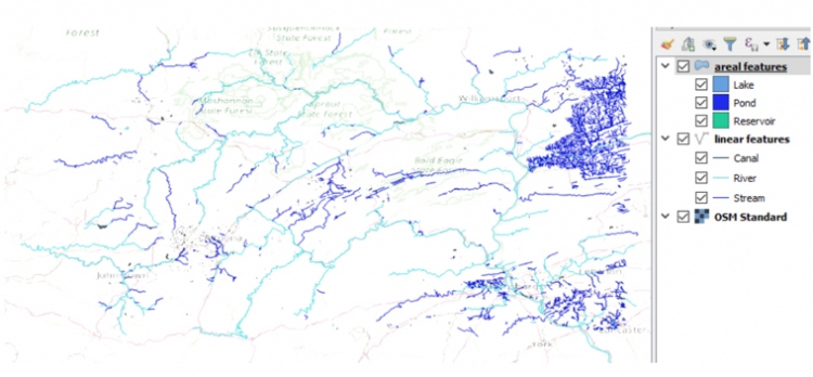
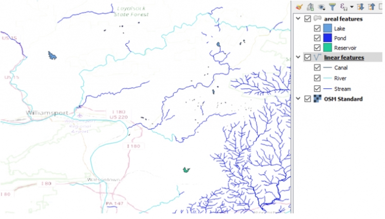
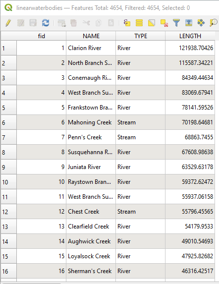
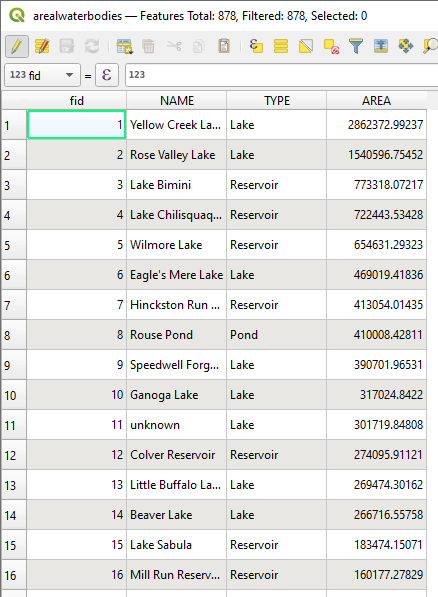
Details
Waterbody class hierarchy:
The classes for the different waterbody types should be arranged in a class hierarchy that looks as in the image below (similar to the bus event hierarchy from the lesson walkthroughs, see also Section 4.7 again). In the end, there should be definitions for all these 9 classes and the different instance variables, methods, and static class functions should be defined at the most suitable locations within the hierarchy. A template file for this class hierarchy that already contains (partial) definitions of some of the classes will be provided below as a starting point.
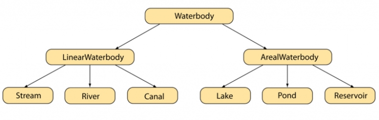
Here are a few requirements for the class hierarchy:
- The entire class hierarchy should be defined in its own file, similar to the bus_events.py file in the lesson walkthroughs.
- Each waterbody object should have an instance variable called name for storing the name of this waterbody, e.g., 'Wilmore Lake'. If there is no “name” tag in the JSON code, the name should be set to “unknown”.
- Each waterbody object should have an instance variable called geometry for storing the geometry of the waterbody as a qgis QgsGeometry object. You will have to create this geometry from the node lists of a way using either the fromPolylineXY(…) or fromPolygonXY(…) functions defined in the QgsGeometry class depending on whether we are dealing with a linear or areal waterbody (see examples from the lesson content, e.g. Section 4.10.2.4). Both functions take QgsPointXY objects as input but in the case of fromPolylineXY(…) it's a single list of QgsPointXY objects, while for fromPolygonXY(...) it's a list of lists of QgsPointXY objects because the polygons can in principle contain polygonal holes.
- Each object of a linear waterbody class should have an instance variable called length for storing its length in meters, while each object of an areal waterbody class should have an instance variable called area for storing its area in square meters. The values for these instance variables can be computed using the approach shown under “Hint 2” below once the geometry object has been created from the nodes. This is already implemented in template class hierarchy file provided below.
- There should be a static class function (see Section 4.8) fromOSMWay(way, allNodes) for all waterbody classes that takes the Python data structure for a single OSM way element and the dictionary containing all OSM node elements read from the input file as parameters. The function then checks the tags of the given way element to see whether or not this element describes a waterbody of the given class and if so creates and returns a corresponding object of that class. For example: If fromOSMWay(way, allNodes) is called for class Stream, the implementation of this function in class Stream needs to check whether or not the tags match the rules for the Stream class (see tag rule list given below). If yes, it will then create a polyline geometry from the node ID list included in the way element by looking up the coordinates for each node in the allNodes dictionary. Then it will create an object of class Stream with the created geometry and, if available, name extracted from the “name” tag of the way. If the tags do not match the rule for Stream, the function simply returns None, signaling that no object was created. Overall this function should work and be used similarly to the detect(…) class functions of the bus event classes from the lesson walkthroughs. The following code provides a basic example of how the function could be used and tested:
import waterbodies                               # import the file with the waterbodies class hierarchy
classes = [ waterbodies.Stream ]                 # list of bottom level classes from the waterbodies.py file; we just use the Stream class in this example but the list can later be extended
way1 = waysDict[5004497]                         # we just work with two particular way elements from our waysDict dictionary in this example; this one is actually a stream ...
way2 = waysDict[4251261]                         # ... while this one is not a stream

for cl in classes:                               # go through the classes in the class list
     print('way1:')
     result = cl.fromOSMWay(way1, nodesDict)     # call the fromOSMWay(...) static class function of the given class providing a way element and our nodes dictionary as parameters;
                                                 # the task of the function is to check whether the way element in the first parameter satisfies the tag rules for the class (e.g. for Stream) and,
                                                 # if yes, create a new object of that class (e.g. an object of class Stream) and return it. To create the object, the function has to create a QgsGeometry
                                                 # object from the list of node IDs listed in the way element first which involves looking up the coordinates of the nodes in the nodes dictionary provided
                                                 # in the second parameter

     if result:                                  # test whether the result is not None meaning that the tag rules for the class were satisfied and an object has been created and returned
         print('object created: ' + str(result)) # since way1 is indeed a Stream this will print out some information about the created object
     else:
         print('return value is None -> no object of class ' + str(cl) + ' has been created')

     print('way2:')
     result = cl.fromOSMWay(way2, nodesDict)     # now we do the same for way2 which is NOT a stream
     if result:                                  # test whether the result is not None meaning that the tag rules for the class were satisfied and an object has been created and returned
         print('object created: ' + str(result))
     else:
         print('return value is None -> no object of class ' + str(cl) + ' has been created') # since way2 is not a stream, this line will be executed
Of course, you will only be able to test run this piece of code once you have implemented the fromOSMWay(...) static class function for the Stream class in the waterbodies class hiearchy file. But here is what the output will look like:way1: object created: <waterbodies.Stream object at 0x000000F198A2C4E0> way2: return value is None -> no object of class <class 'waterbodies.Stream'> has been created
Also, the idea of course is that later fromOSMWay(...) will be called for all way elements in the waysDict dictionary, not for particular elements like we are doing in this example. - There should be a method toQgsFeature(self) that can be invoked for all waterbody objects. This method is supposd to create and return a QgsFeature object for the waterbody object it is invoked on. The returned QgsFeature object can then be added to one of the output GeoPackage files. When called for an object of a linear waterbody class, the created feature should have the polyline geometry of that object and at least the attributes NAME, TYPE, and LENGTH as shown in the image of the linear attribute table above. When called for an areal waterbody class, the created feature should have the polygon geometry of that object and at least the attributes NAME, TYPE, and AREA (see the image with the areal attribute table above). Using this method to create a QgsGeometry object can be integrated into the for-loop of the example code from the previous point:
    if result:                          # test whether the result is not None meaning the tag rules for class where satisfied an object has been created and returned
        feature = result.toQgsFeature() # call toQgsFeature() to create a QgsFeature object from the waterbody object
        print(feature)                  # print string representation of feature
        print(feature.attributes())     # print attribute values as a list
        # do something else with feature like storing it somewhere for later use
Assuming this code is executed for way1, running the code after the toQgsFeature() method has been implement should produce the following output:<qgis._core.QgsFeature object at 0x000000AB6E36F8B8> ['Rapid Run', 'Stream', 372.01922201444535]
The attributes listed are the name, the type, and the length of the stream. - Add a definition of the __str__(self) method to each class at the bottom level of the hierarchy with the goal of producing a nicer description of the object than simply something like <waterbodies.Stream object at 0x000000F198A2C4E0>. The description should include the type, name, and length/area of the object, so for example it could look like this:
Stream Rapid Run (length: 372.01922201444535m)
While this method will not play an important role in the final version of the code for this assignment, it can be very useful to provide some helpful output for debugging. Keep in mind that, once you have defined this method, using print(result) or str(result) in the code examples for fromOSMWay(...) will produce this more readable and more informative description instead of just <waterbodies.Stream object at 0x000000F198A2C4E0>.
Tag rules for different waterbodies
We already mentioned that we are providing the tag rules for the six bottom-level classes in the hierarchy that should be used for checking whether or not a given OSM way describes an instance of that class. You simply will have to turn these into Python code in the different versions of the fromOSMWay(way, allNodes) static class function in your class hierarchy. Here are the rules:
Stream: the way has the “tags” attribute and among the tags is the key “waterway” with the value “stream” assigned.
River: the way has the “tags” attribute and among the tags is the key “waterway” with the value “river” assigned.
Canal: the way has the “tags” attribute and among the tags is the key “waterway” with the value “canal” assigned.
Lake: the way has the “tags” attribute and among the tags there is both, the key “natural” with the value “water” assigned and the key “water” with the value “lake” assigned.
Pond: the way has the “tags” attribute and among the tags there is both, the key “natural” with the value “water” assigned and the key “water” with the value “pond” assigned.
Reservoir: the way has the “tags” attribute and among the tags there is both, the key “natural” with the value “water” assigned and the key “water” with the value “reservoir” assigned.
Right now, the rules for all three linear classes are the same except for the specific value that needs to be assigned to the “waterway” key. Similarly, the rules for all three areal classes are the same except for the specific value that needs to be assigned to the “water” key. However, since these rules may change, the logic for checking the respective conditions should be implemented in the fromOSMWay(way, allNodes) class function for each of these six classes.
Creation of output GeoPackage files:
You saw examples of how to create new layers and write them to GeoPackage files with qgis in Section 4.5.3 and the lesson walkthrough code from Section 4.10 (main.py and bus_track_analyzer.py). So once you have gone through the list of way elements in the input data and created waterbody objects of the different classes via the fromOSMWay(...) static class functions, creating the features by calling the toQgsFeature() method of each waterbody object and producing the output files should be relatively easy and just require a couple lines of code. You will have to make sure to use the right geometry type and CRS when creating the layers with qgis.core.QgsVectorLayer(...) though.
GUI:
As in the Lesson 2 assignment, you are again free to design the GUI for your tool yourself. The GUI will be relatively simple but you can extend it based on what you learned in this lesson for over&above points. The GUI should look professional and we are providing a minimal list of elements that need to be included:
- A combination of a line edit widget and tool button that opens a file dialog for allowing the user to select the input JSON file.
- Similar combinations of widgets for choosing the names under which the two new output GeoPackage files should be saved with a "save file" dialog.
- A button that starts the process of reading the data, going through the way elements and creating the waterbody objects, creating the two new GeoPackage output files and populating them with the QgsFeature objects created from the waterbody objects.
- Optional for over&above points: A QWidget for displaying information about how many features of the six different classes have been created as shown in the image below using drawing operations as explained in Section 4.9.1 and used in the lesson walkthrough. A basic version of this widget would just display the names and numbers here. Showing bars whose width indicates the relative percentages of the different waterbody types is an option for more over&above points. The class for this widget should be defined in its own file, similar to the class BusTrackerWidget in the lesson walkthrough.
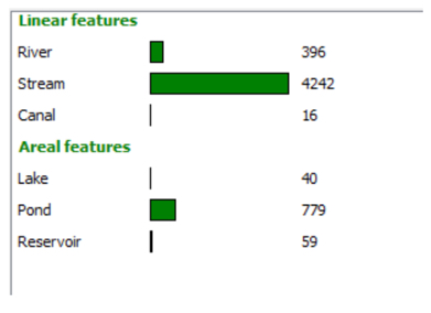
Class hierarchy template file:
If you think you have a good grasp on the fundamentals of object-oriented programming in Python, we recommend that you challenge yourself and try to develop your own solution for this assignment from scratch. However, for the case that you feel a bit overwhelmed by the task of having to implement the class hierarchy yourself, we are here providing a draft file for the waterbody class hierarchy [54] that you can use as a starting point. The file contains templates for the definitions of the classes from the leftmost branch of the hierarchy, so the classes Waterbody, LinearWaterbody and Stream, as well as the ArealWaterbody class. Your first task will then be to understand the definitions and detailed comments, and then add the missing parts needed to complete the definition of the Stream class such as the code for testing whether or not the tag rules for Streams are satisfied, for producing the polyline geometry, and for creating a QgsFeature. The class definition of Stream in particular contains detailed comments on what steps need to be implemented for fromOSMWay(...) and toQgsFeature().
You can then test your implementation by adapting the code examples given above to put together a main program that reads in the data from the JSON input file, calls the fromOSMWay(...) function of the Stream class for each way element, and collects the Stream objects produced from this. You can then either print out the information (name, length) from the instance variables of the Stream objects directly to see whether or not the output makes sense or you next implement the __str__(self) method for Stream to produce the same kind of output with print(result). Then go one step further and write the code for producing a GeoPackage file with the QgsFeature objects produced from calling the toQgsFeature() method for each Stream object that has been created.
Once you have this working for the Stream class, you can start to add the other classes from the hierarchy. You will see that these need to be defined very similarly to the Stream class, so you will only have to make smaller modifications and extensions. Once the full hierarchy is working and you are able to produce the correct GeoPackage files, the final part will be to design and incorporate the GUI.
As a last comment, if you want to make changes to the existing code in the template file, that is absolutely ok; please don't treat it as something that you have to use in exactly this way. There are many possible ways in which this assignment can be solved and this draft follows one particular approach. However, the fromOSMWay(way, allNodes) static class function and toQgsFeature(self) method need to appear in the class definitions with exactly the given paramters, so this is something you are not allowed to change.
Overall, the main.py file and the general file organization of the walkthrough code in Section 4.10 provide a good template for this assignment but no worries, this assignment is significantly simpler and requires much less code. Below you can find two more hints on some of the steps involved.
Hint 1
In the lesson walkthrough, we had a list with the names of all bus event classes that we were looking for in the data. We then used a for-loop to go through that list and call the detect(…) class function for each class in the list. In this assignment, it may make more sense to have two separate lists: one for the class names of the linear waterbody classes and one for the names of the areal waterbody classes. That is because you probably would want to store the objects of both groups in separate lists since they need to be added to two different output files.
Hint 2
If you are using the template class hierarchy file, you won't have to write this code yourself but the following will help you understand what is going on with the length and area computation code: when we have a QgsGeometry object in variable geometry, we can calculate its length/area with the help of an object of the qgis QgsDistanceArea class. We first set up a QgsDistanceArea object suitable for WGS84 coordinates:
qda = qgis.core.QgsDistanceArea()

qda.setEllipsoid('WGS84')
Then we calculate the length or area (depending on whether the geometry is a polyline or polygon) with:
length = qda.measureLength(geometry)
or
area = qda.measureArea(geometry)
Finally, we convert the area or length number into the measurement unit we want, e.g. with
lengthMeters = qda.convertLengthMeasurement(length, qgis.core.QgsUnitTypes.DistanceMeters)
or
areaSquareMeters = qda.convertAreaMeasurement(area, qgis.core.QgsUnitTypes.AreaSquareMeters)
Grading Criteria
The criteria your code submission will be graded on will include how elegant your code is and how well you designed the class hierarchy as well as how well-designed the GUI of your tool is. Successful completion of the above requirements and the write-up discussed below is sufficient to earn 90% of the credit on this project. The remaining 10% is reserved for "over and above" efforts which could include, but are not limited to, the following (the last two options are significantly more difficult and require more work than the first two, so more o&a points will be awarded for these):
- Look through the JSON for some other types of waterbodies (linear or areal ones) that appear there. Pick one and add it to your tool by adding a corresponding class to the waterbody class hierarchy and changing the code so that ways of that class are detected as well.
- Add some code to your tool that first sorts all linear waterbody objects by decreasing length and all areal waterbody objects by decreasing area before adding the objects to the data set. As a result, the order should be as shown in the attribute table images above without first having to sort the rows in QGIS. For this, you should override the < operator by defining the __lt__(self, otherObject) method (for “less than”) for these classes so that it compares the lengths/areas of the two involved objects. You can then simply use the list method sort(…) for a list with all linear/areal objects to do the sorting.
- Add the information display widget showing numbers of objects created for the different classes using QPainter methods to the GUI of your program as described above. The advanced version with bar chart as shown in the image above is sufficient to earn full o&a points if done well.
- Turn the standalone tool into a QGIS plugin that adds the produced data sets as new layers to the project currently open in QGIS using a dock widget as in Section 4.12 (this option alone will give full o&a points if done well).
Write-up
Produce a 400-word write-up on how the assignment went for you; reflect on and briefly discuss the issues and challenges you encountered and what you learned from the assignment. Please also briefly mention what you did for "over and above" points in the write-up.
Deliverable
Submit a single .zip file to the corresponding drop box on Canvas; the zip file should contain:
- The folder with the entire code for your tool
- Your 400-word write-up