Overview

To forecast the weather, we use numerical weather prediction models that are based on mathematical expressions for conservation of energy, mass, and momentum. Climate prediction models are based on the same conservation laws. Conservation simply means that the amount of a quantity such as total energy, mass, or momentum remains constant even though the forms of that quantity may change. Conservation of energy is described by the 1^st Law of Thermodynamics, which was discussed in Lesson 2; conservation of mass and conservation of momentum are discussed in this lesson. The total mass of an air parcel is constant, but density and volume may change. The conservation of momentum is based on Newton's 2^nd Law and involves forces that can change momentum. The conservation of momentum is relatively simple when cast in an inertial (non-accelerating) reference frame because there are only three real forces that really matter for atmospheric motion: gravity, the pressure gradient force, and friction. But when cast on a rotating Earth, we need to add apparent forces to this equation in order to compensate for the fact that an air parcel on Earth is always accelerating as the Earth rotates. We end up adding the apparent forces—Coriolis force and centrifugal force—to the real forces to get an equation of motion whose predictions we can readily match with our observations.

Some atmospheric motion occurs with air masses and waves that are thousands of kilometers across, while other motion, such as tornadoes, is at most a few kilometers across. Sometimes air flows in a straight line; sometimes it flows around ridges and troughs. In all of these different cases, the most important forces are different, allowing the momentum conservation equation to be simplified in different ways. We will discuss these different conditions and show how you can determine the wind velocity from knowledge of the balance of the most important forces and thus determine the impact of air motion at upper levels on the air motion near Earth’s surface. Finally, we will describe why midlatitude winds are westerly.

Learning Objectives

By the end of this lesson, you should be able to:

• explain mass conservation physically, recognize the mass conservation equation, and memorize its form when density is constant
• state the three main conservation laws in atmospheric science: the conservation of mass, the conservation of momentum, and the conservation of energy
• name and explain the three fundamental (real) forces in the atmosphere (gravity, pressure gradient, and friction)
• name and explain the two new (apparent) forces that emerge when momentum conservation is written in the rotating reference frame
• draw the balance of forces for geostrophic flow, gradient flow, geostrophic flow with friction, and cyclostrophic flow
• explain why midlatitude winds are westerly

Questions?

If you have any questions, please post them to the Course Questions discussion forum. I will check that discussion forum daily to respond. While you are there, feel free to post your own responses if you, too, are able to help out a classmate.

10.1 Why We Like Conservation

Scientists like things that are conserved. There are good reasons for this. First, if something is conserved, that means we can always count on it being the same no matter what happens. Second, when we write down the equation for the conserved quantity, we can use that equation to understand how the equation’s variables will change with differing conditions. For example, in Lesson 2, we were able to use the First Law of Thermodynamics (a.k.a., conservation of energy) along with the Ideal Gas Law to derive the equation for potential temperature, which is very useful for understanding and calculating the vertical motion of air parcels.

In atmospheric dynamics, we like three conservation laws:

1. conservation of energy (The 1^st Law of Thermodynamics [1])
2. conservation of mass
3. conservation of momentum (Newton’s Second Law, but really three equations—one in each direction)

Conservation of Mass

So, let’s step back and look at the mass of an air parcel, which equals the density times the volume of the parcel:

In a parcel, the mass is conserved, and since m = ρV,

Apply the product rule to Equation [10.2]:

Divide both sides by ρV:

Recall that the specific rate of change in parcel volume is equal to the divergence (Equation 9.4) and so we can write:

Rearranging the equation gives us an expression for the conservation of mass:

This equation is for the conservation of mass in a continuous fluid (i.e., the fluid particles are so small that the air parcel behaves like a fluid). It is also called the Equation of Continuity. Physically, this equation means that if the flow is converging ($\overrightarrow{\nabla }•\overrightarrow{U}<0$[2]@5@5@+=faaagCart1ev2aqaKnaaaaWenf2ys9wBH5garuavP1wzZbItLDhis9wBH5garmWu51MyVXgaruWqVvNCPvMCG4uz3bqee0evGueE0jxyaibaieYlNi=xH8yiVC0xbbL8FesqqrFfpeea0xe9Lq=Jc9vqaqpepm0xbbG8FasPYRqj0=yi0dXdbba9pGe9xq=JbbG8A8frFve9Fve9Ff0dc9Gqpi0dmeaabaqaciGacaGaaeqabaWaaeaaeaaakeaaqaaaaaaaaaWdbmaaFiaabaGaey4bIenacaGLxdcacaGGIaYaa8HaaeaacaWGvbaacaGLxdcacqGH8aapcaaIWaaaaa@3B2C@ ), then the density must increase ($\frac{D\rho }{Dt}$[2]@5@5@+=faaagCart1ev2aqaKnaaaaWenf2ys9wBH5garuavP1wzZbItLDhis9wBH5garmWu51MyVXgaruWqVvNCPvMCG4uz3bqee0evGueE0jxyaibaieYlNi=xH8yiVC0xbbL8FesqqrFfpeea0xe9Lq=Jc9vqaqpepm0xbbG8FasPYRqj0=yi0dXdbba9pGe9xq=JbbG8A8frFve9Fve9Ff0dc9Gqpi0dmeaabaqaciGacaGaaeqabaWaaeaaeaaakeaaqaaaaaaaaaWdbmaalaaapaqaa8qacaWGebGaeqyWdihapaqaa8qacaWGebGaamiDaaaaaaa@3779@ >0). Note that in Lesson 9.5 [3]we said that density doesn’t change much at any fixed pressure level, which is how we were able to relate horizontal divergence/convergence with vertical ascent/descent. What did change was the vertical size of the air parcel as the horizontal size increased or decreased. The total mass, however, remained the same.

"Isaac Newton woodcut, frontispiece to Mach" by an unknown artist after a portrait by Kneller, ca. 1689.

Credit: Licensed under Public Domain via Wikimedia Commons [4]

Conservation of Momentum

Newton’s 2^nd Law, F = ma, applies to a mass with respect to the inertial coordinate system of space. But we are interested in motion with respect to the rotating Earth. So, to apply Newton’s 2^nd Law to Earth’s atmosphere, our mathematics will need to account for the forces of Earth’s rotating coordinate system:

where the first set of forces are real forces and the second set are apparent (or effective) forces that will be used to correct for using a coordinate system attached to a rotating Earth.

When we use the word “specific” as an adjective describing a noun in science, we mean that noun divided by mass. So, specific force is F/m = a, acceleration. In what follows, we will use the terms “force” and “acceleration” interchangeably, assuming that if we say “force,” we mean “force/mass,” which is acceleration. At this point, you should be able to check the units—if there is no “kg,” then obviously we are talking about accelerations.

10.2 What are the important real forces?

There are three real forces important for atmospheric motion:

1. Gravitational Force
2. Pressure Gradient Force (PGF)
3. Friction

Hence we can sum these real forces:

We put the subscript "a" on these forces to indicate "absolute" because they are true in an inertial reference frame. Thus, in the absolute reference frame,

Let's examine each of these real forces in more detail.

1. Gravitational Force

Recall that the gravitational force on a mass m is simply the weight of the mass, which is given by:

where M is Earth’s mass (5.9722 x 10²⁴ kg), $\overrightarrow{r}$[2]@5@5@+=faaahmart1ev3aaaKnaaaaWenf2ys9wBH5garuavP1wzZbItLDhis9wBH5garmWu51MyVXgaruWqVvNCPvMCaebbnrfifHhDYfgasaacH8srps0lbbf9q8WrFfeuY=ribbf9v8qqaqFr0xc9pk0xbba9q8WqFfea0=yr0RYxir=Jbba9q8aq0=yq=He9q8qqQ8frFve9Fve9Ff0dc9Gqpi0dmeaabaqaciGacaGaaeqabaWaaeaaeaaakeaaceWGYbGbaSaaaaa@3287@  is the distance vector originating from the Earth’s center, and G is the gravitational constant (6.6741 × 10^–11 m³ kg^–1 s^-2). Ignoring the minor effects of topography and the horizontal variation of Earth's density, the real gravitational force points directly towards Earth’s center. The gravitational force per unit mass is simply $\overrightarrow{g}*$[2]@5@5@+=faaagCart1ev2aqaKnaaaaWenf2ys9wBH5garuavP1wzZbItLDhis9wBH5garmWu51MyVXgaruWqVvNCPvMCG4uz3bqee0evGueE0jxyaibaieYlf9irVeeu0dXdh9vqqj=hHeeu0xXdbba9frFj0=OqFfea0dXdd9vqaq=JfrVkFHe9pgea0dXdar=Jb9hs0dXdbPYxe9vr0=vr0=vqpi0dc9GqpWqaaeaabiGaciaacaqabeaadaqaaqaaaOqaamaaFiaabaGaam4zaaGaay51GaGaaiOkaaaa@3619@ .

2. Pressure Gradient Force (PGF)

The derivation of the pressure gradient force is similar to what we have already done in Lesson 2.2 to find hydrostatic equilibrium [5], except that we will look at only the pressure forces in this case, and will serve as a quick review. Consider the x-direction first:

Drawing of the forces involved in the pressure gradient force in the x direction.

Credit: W. Brune

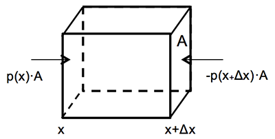
Adding in the y and z directions, we get the 3-D vector form of the pressure gradient force per unit mass:

Example

Let's do a quick calculation of the pressure gradient force from a map of surface pressure on 26 June 2015. Note that Pennsylvania's northern border is about 250 km from its southern border.

Click here for an accessible alternative to the text on the image

Reads: PA is ~250 km high. Isobars are 4 mb apart. Air density ~1.2kg/m³. From 1008 mb isobar to 1016 mb isobar is ~300 km. |PGF| = (1/1.2)* (800 Pa/(300*1000) = 2.2x10^-3 m s^-2 pointing due west

Credit: Penn State e-Wall and W. Brune

3. Friction

We can think of friction as being processes that impede the airflow. There are two different types of friction that meteorologists are concerned with: molecular friction and turbulent friction. Molecular friction is a real force that appears in the conservation of momentum equation whereas turbulent friction is an additional term that arises out of averaging the conservation of momentum equation.

Molecular friction results from the random movement of molecules. Imagine two air parcels moving towards the east. One air parcel is just to the north of the other and is moving a bit faster than the other. Due to random molecular motion, the two parcels exchange air molecules that carry the momentum of their respective air parcels. When molecules collide, some of their momentum is transferred, resulting in the faster parcel (the one to the north) slowing down and the slower parcel (the one to the south) speeding up. There is thus a transfer of momentum from the faster parcel to the slower parcel. This transfer is proportional to the velocity difference between the air parcels and a quantity called the viscosity. The viscosity depends on the fluid in question (air in this case) and the temperature. Fluids with a relatively high resistance to motion, like honey, have relatively high viscosities. Think about air near the Earth's surface. The air right at the surface is stationary due to electromagnetic forces between the air and the surface. Due to molecular friction, the air near the surface will slow down the air just above it, just as that air slows the air a little bit higher. We show without derivation that the molecular friction force (sometimes called the viscous force) per unit mass is to a very good approximation given by:

$$\frac{{\overrightarrow{F}}_f}{m}=\nu {\nabla }^2{\overrightarrow{U}}_a$$[2]@5@5@+=faaahmart1ev3aaaKnaaaaWenf2ys9wBH5garuavP1wzZbItLDhis9wBH5garmWu51MyVXgaruWqVvNCPvMCaebbnrfifHhDYfgasaacH8srps0lbbf9q8WrFfeuY=ribbf9v8qqaqFr0xc9pk0xbba9q8WqFfea0=yr0RYxir=Jbba9q8aq0=yq=He9q8qqQ8frFve9Fve9Ff0dc9Gqpi0dmeaabaqaciGacaGaaeqabaWaaeaaeaaakeaaqqaaaaaaaaGySf2yRbWdbmaalaaapaqaa8qaceWGgbWdayaalaWaaSbaaSqaa8qacaWGMbaapaqabaaakeaapeGaamyBaaaacqGH9aqpcqaH9oGBcaaMc8Uaey4bIe9damaaCaaaleqabaWdbiaaikdaaaGcceWGvbWdayaalaWdbmaaBaaaleaacaWGHbaabeaaaaa@3FFA@

where ν is the kinematic viscosity, ${\nabla }^2=\overrightarrow{\nabla }·\overrightarrow{\nabla }=\frac{{\partial }^2}{\partial x^2}+\frac{{\partial }^2}{\partial y^2}+\frac{{\partial }^2}{\partial z^2}$ is called the Laplace operator or the Laplacian, and $\overrightarrow{U}$ is the air parcel velocity. The viscous force is important for resisting flow and dissipating air flow on small scales, such as for an individual raindrop, but it is not an important force on larger scales when compared to other forces such as gravity and the pressure gradient force (as will be demonstrated in Lesson 10.5).

Turbulent friction is important for larger-scale atmospheric motion, even synoptic-scale motion. The flow in the atmosphere's lowest kilometer or two, called the atmospheric boundary layer is often turbulent, with chaotic large and small swirls of air that, when taken together, have momentum in all directions. During the day, turbulence is generated by convection. During both day and night, turbulence is also generated by wind shear throughout the boundary layer. No matter how turbulence is generated, it provides a drag on the horizontal flow throughout the boundary layer because upward moving air with low horizontal momentum collides with air aloft with high horizontal momentum, slowing it down. This turbulent drag is often referred to as friction, even though the word "friction" really applies only to molecular-scale interactions.

Turbulent friction is not a fundamental force; it is represented in the conservation of momentum equation only after the equation has been averaged over time, space, or both. New terms representing turbulent friction arise from the averaging of the advective derivative, which we will discuss in more detail in Lesson 11. For now, we take the momentum conservation equation and average it so that all of the quantities that we are predicting—like velocity, pressure, and density—really reflect average quantities that vary gradually over space and time. For example, the wind velocity averaged over an hour and over the southeastern quarter of Pennsylvania would be a good example of a quantity one could predict from the averaged momentum conservation equation. On the other hand, a wind gust measured by an anemometer on top of a building would not be a good example of such a quantity.

For a turbulent boundary layer, the turbulent friction per unit mass is a function of four quantities: the dimensionless drag coefficient C_d, the planetary boundary layer height h, the magnitude of the horizontal velocity $\left|{\overrightarrow{V}}_a\right|$[2]@5@5@+=faaahmart1ev3aaaKnaaaaWenf2ys9wBH5garuavP1wzZbItLDhis9wBH5garmWu51MyVXgaruWqVvNCPvMCaebbnrfifHhDYfgasaacH8srps0lbbf9q8WrFfeuY=ribbf9v8qqaqFr0xc9pk0xbba9q8WqFfea0=yr0RYxir=Jbba9q8aq0=yq=He9q8qqQ8frFve9Fve9Ff0dc9Gqpi0dmeaabaqaciGacaGaaeqabaWaaeaaeaaakeaaqqaaaaaaaaGySf2yRbWdbmaaemaapaqaa8qaceWGwbWdayaalaWdbmaaBaaaleaacaWGHbaabeaaaOGaay5bSlaawIa7aaaa@3908@ , and the horizontal velocity itself:

Even though this turbulent drag is not really friction, it is an important resistance to the average horizontal flow on large scales in the boundary layer and so we will keep it, and not molecular friction, as the friction term in the averaged momentum equation. Note that the turbulent drag is greatest within the boundary layer and becomes much smaller above the boundary layer, where it is assumed that the drag coefficient becomes very small.

10.3 Effects of Earth’s Rotation: Apparent Forces

Newton’s Second Law applies in an inertial reference frame, which means that the reference frame is not accelerating. A point on the rotating Earth is not following a straight line through space, but instead follows a roughly circular path and hence is constantly accelerating towards the axis of rotation. Therefore, Earth does not provide an inertial reference frame. For an astronaut in distant space observing the weather on Earth, the air motions obey Newton’s Second Law perfectly, but for an Earth-bound observer, Newton’s Second Law fails to capture the observed motion. To account for this crazy behavior, the Earth-bound observer needs to add some apparent forces to the real forces for the math to explain the observed motion from the point of view of someone standing on the rotating Earth.

Earth’s rotation is to the east. The symbol ⨂ indicates that the vector ${\overrightarrow{U}}_e$[2]@5@5@+=faaagCart1ev2aaaKnaaaaWenf2ys9wBH5garuavP1wzZbItLDhis9wBH5garmWu51MyVXgaruWqVvNCPvMCG4uz3bqee0evGueE0jxyaibaieYlf9irVeeu0dXdh9vqqj=hHeeu0xXdbba9frFj0=OqFfea0dXdd9vqaq=JfrVkFHe9pgea0dXdar=Jb9hs0dXdbPYxe9vr0=vr0=vqpi0dc9GqpWqaaeaabiGaciaacaqabeaadaqaaqaaaOqaamaaFiaabaGaamOvaaGaay51GaWaaSbaaSqaaiaadwgaaeqaaaaa@366F@ is going into the page with a magnitude RΩ.

Credit: W. Brune

Suppose we have an air parcel moving through space with a velocity ${\overrightarrow{U}}_a$[2]@5@5@+=faaagCart1ev2aaaKnaaaaWenf2ys9wBH5garuavP1wzZbItLDhis9wBH5garmWu51MyVXgaruWqVvNCPvMCG4uz3bqee0evGueE0jxyaibaieYlf9irVeeu0dXdh9vqqj=hHeeu0xXdbba9frFj0=OqFfea0dXdd9vqaq=JfrVkFHe9pgea0dXdar=Jb9hs0dXdbPYxe9vr0=vr0=vqpi0dc9GqpWqaaeaabiGaciaacaqabeaadaqaaqaaaOqaamaaFiaabaGaamOvaaGaay51GaWaaSbaaSqaaiaadggaaeqaaaaa@366B@, which we will call the absolute velocity. We want to relate this absolute velocity to $\overrightarrow{U}$[2]@5@5@+=faaagCart1ev2aaaKnaaaaWenf2ys9wBH5garuavP1wzZbItLDhis9wBH5garmWu51MyVXgaruWqVvNCPvMCG4uz3bqee0evGueE0jxyaibaieYlf9irVeeu0dXdh9vqqj=hHeeu0xXdbba9frFj0=OqFfea0dXdd9vqaq=JfrVkFHe9pgea0dXdar=Jb9hs0dXdbPYxe9vr0=vr0=vqpi0dc9GqpWqaaeaabiGaciaacaqabeaadaqaaqaaaOqaamaaFiaabaGaamOvaaGaay51Gaaaaa@3559@, the velocity observed with respect to the Earth reference frame. Let ${\overrightarrow{U}}_e$[2]@5@5@+=faaagCart1ev2aaaKnaaaaWenf2ys9wBH5garuavP1wzZbItLDhis9wBH5garmWu51MyVXgaruWqVvNCPvMCG4uz3bqee0evGueE0jxyaibaieYlf9irVeeu0dXdh9vqqj=hHeeu0xXdbba9frFj0=OqFfea0dXdd9vqaq=JfrVkFHe9pgea0dXdar=Jb9hs0dXdbPYxe9vr0=vr0=vqpi0dc9GqpWqaaeaabiGaciaacaqabeaadaqaaqaaaOqaamaaFiaabaGaamOvaaGaay51GaWaaSbaaSqaaiaadwgaaeqaaaaa@366F@ be the velocity of the Earth. Here we only consider the velocity of the Earth due to rotation about its axis (the motion around the Sun is much less important), so ${\overrightarrow{U}}_e$[2]@5@5@+=faaagCart1ev2aaaKnaaaaWenf2ys9wBH5garuavP1wzZbItLDhis9wBH5garmWu51MyVXgaruWqVvNCPvMCG4uz3bqee0evGueE0jxyaibaieYlf9irVeeu0dXdh9vqqj=hHeeu0xXdbba9frFj0=OqFfea0dXdd9vqaq=JfrVkFHe9pgea0dXdar=Jb9hs0dXdbPYxe9vr0=vr0=vqpi0dc9GqpWqaaeaabiGaciaacaqabeaadaqaaqaaaOqaamaaFiaabaGaamOvaaGaay51GaWaaSbaaSqaaiaadwgaaeqaaaaa@366F@ is always eastward, greatest at the equator and zero at the poles. The absolute velocity of an air parcel is simply the velocity of the air parcel with respect to the Earth plus the velocity of the Earth itself: ${\overrightarrow{U}}_a=\overrightarrow{U}+{\overrightarrow{U}}_e$[2]@5@5@+=faaahmart1ev3aaaKnaaaaWenf2ys9wBH5garuavP1wzZbItLDhis9wBH5garmWu51MyVXgaruWqVvNCPvMCaebbnrfifHhDYfgasaacH8srps0lbbf9q8WrFfeuY=ribbf9v8qqaqFr0xc9pk0xbba9q8WqFfea0=yr0RYxir=Jbba9q8aq0=yq=He9q8qqQ8frFve9Fve9Ff0dc9Gqpi0dmeaabaqaciGacaGaaeqabaWaaeaaeaaakeaaqqaaaaaaaaGySf2yRbWdbiqadwfapaGbaSaadaWgaaWcbaWdbiaadggaa8aabeaakiabg2da98qaceWGvbWdayaalaGaey4kaSYdbiqadwfapaGbaSaadaWgaaWcbaWdbiaadwgaa8aabeaaaaa@3B08@

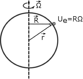
What is the velocity of the Earth? Consider a specific point on the Earth. Let $\overrightarrow{\Omega }$[2]@5@5@+=faaagCart1ev2aqaKnaaaaWenf2ys9wBH5garuavP1wzZbItLDhis9wBH5garmWu51MyVXgaruWqVvNCPvMCG4uz3bqee0evGueE0jxyaibaieYlf9irVeeu0dXdh9vqqj=hHeeu0xXdbba9frFj0=OqFfea0dXdd9vqaq=JfrVkFHe9pgea0dXdar=Jb9hs0dXdbPYxe9vr0=vr0=vqpi0dc9GqpWqaaeaabiGaciaacaqabeaadaqaaqaaaOqaamaaFiaabaGaeuyQdCfacaGLxdcaaaa@360D@ be Earth’s angular velocity vector, $\overrightarrow{r}$[2]@5@5@+=faaagCart1ev2aqaKnaaaaWenf2ys9wBH5garuavP1wzZbItLDhis9wBH5garmWu51MyVXgaruWqVvNCPvMCG4uz3bqee0evGueE0jxyaibaieYlf9irVeeu0dXdh9vqqj=hHeeu0xXdbba9frFj0=OqFfea0dXdd9vqaq=JfrVkFHe9pgea0dXdar=Jb9hs0dXdbPYxe9vr0=vr0=vqpi0dc9GqpWqaaeaabiGaciaacaqabeaadaqaaqaaaOqaamaaFiaabaGaamOCaaGaay51Gaaaaa@3576@ be the position vector from the Earth’s center to the point in question, and $\overrightarrow{R}$ be the shortest distance vector from the axis of rotation to the point in question (as in the figure above). The magnitude of $\overrightarrow{\Omega }$[2]@5@5@+=faaagCart1ev2aqaKnaaaaWenf2ys9wBH5garuavP1wzZbItLDhis9wBH5garmWu51MyVXgaruWqVvNCPvMCG4uz3bqee0evGueE0jxyaibaieYlf9irVeeu0dXdh9vqqj=hHeeu0xXdbba9frFj0=OqFfea0dXdd9vqaq=JfrVkFHe9pgea0dXdar=Jb9hs0dXdbPYxe9vr0=vr0=vqpi0dc9GqpWqaaeaabiGaciaacaqabeaadaqaaqaaaOqaamaaFiaabaGaeuyQdCfacaGLxdcaaaa@360D@ is $\left|\overrightarrow{\Omega }\right|=\frac{2\pi }{23.934\text{ hr}}\frac{1\text{ hr}}{3600\text{ s}}=7.292\times {10}^{-5}{\text{s}}^{-\text{1}}$[2]@5@5@+=faaahmart1ev3aaaKnaaaaWenf2ys9wBH5garuavP1wzZbItLDhis9wBH5garmWu51MyVXgaruWqVvNCPvMCaebbnrfifHhDYfgasaacH8srps0lbbf9q8WrFfeuY=ribbf9v8qqaqFr0xc9pk0xbba9q8WqFfea0=yr0RYxir=Jbba9q8aq0=yq=He9q8qqQ8frFve9Fve9Ff0dc9Gqpi0dmeaabaqaciGacaGaaeqabaWaaeaaeaaakeaaqqaaaaaaaaGySf2yRbWdbmaaemaapaqaa8qacuqHPoWvpaGbaSaaa8qacaGLhWUaayjcSdGaeyypa0ZaaSaaa8aabaWdbiaaikdacqaHapaCa8aabaWdbiaaikdacaaIZaGaaiOlaiaaiMdacaaIZaGaaGinaiaabccacaqGObGaaeOCaaaadaWcaaWdaeaapeGaaGymaiaabccacaqGObGaaeOCaaWdaeaapeGaaG4maiaaiAdacaaIWaGaaGimaiaabccacaqGZbaaaiabg2da9iaaiEdacaGGUaGaaGOmaiaaiMdacaaIYaGaey41aqRaaGymaiaaicdapaWaaWbaaSqabeaapeGaeyOeI0IaaGynaaaakiaabohapaWaaWbaaSqabeaapeGaeyOeI0Iaaeymaaaaaaa@5893@ and the direction of $\overrightarrow{\Omega }$[2]@5@5@+=faaagCart1ev2aqaKnaaaaWenf2ys9wBH5garuavP1wzZbItLDhis9wBH5garmWu51MyVXgaruWqVvNCPvMCG4uz3bqee0evGueE0jxyaibaieYlf9irVeeu0dXdh9vqqj=hHeeu0xXdbba9frFj0=OqFfea0dXdd9vqaq=JfrVkFHe9pgea0dXdar=Jb9hs0dXdbPYxe9vr0=vr0=vqpi0dc9GqpWqaaeaabiGaciaacaqabeaadaqaaqaaaOqaamaaFiaabaGaeuyQdCfacaGLxdcaaaa@360D@  is determined by the right hand rule (the direction of your thumb when you curl the fingers of your right hand in the direction of rotation and point your thumb towards the North Star). To determine the angular velocity of the Earth, note that we have used the sidereal day length, 23.934 hr, which is the day length when Earth's rotation is measured with respect to the fixed stars (the inertial reference frame).

The following video (:51) will demonstrate the right hand rule:

The magnitude of ${\overrightarrow{U}}_e$[2]@5@5@+=faaagCart1ev2aaaKnaaaaWenf2ys9wBH5garuavP1wzZbItLDhis9wBH5garmWu51MyVXgaruWqVvNCPvMCG4uz3bqee0evGueE0jxyaibaieYlf9irVeeu0dXdh9vqqj=hHeeu0xXdbba9frFj0=OqFfea0dXdd9vqaq=JfrVkFHe9pgea0dXdar=Jb9hs0dXdbPYxe9vr0=vr0=vqpi0dc9GqpWqaaeaabiGaciaacaqabeaadaqaaqaaaOqaamaaFiaabaGaamOvaaGaay51GaWaaSbaaSqaaiaadwgaaeqaaaaa@366F@ is RΩ, but we need to write ${\overrightarrow{U}}_e$[2]@5@5@+=faaagCart1ev2aaaKnaaaaWenf2ys9wBH5garuavP1wzZbItLDhis9wBH5garmWu51MyVXgaruWqVvNCPvMCG4uz3bqee0evGueE0jxyaibaieYlf9irVeeu0dXdh9vqqj=hHeeu0xXdbba9frFj0=OqFfea0dXdd9vqaq=JfrVkFHe9pgea0dXdar=Jb9hs0dXdbPYxe9vr0=vr0=vqpi0dc9GqpWqaaeaabiGaciaacaqabeaadaqaaqaaaOqaamaaFiaabaGaamOvaaGaay51GaWaaSbaaSqaaiaadwgaaeqaaaaa@366F@ as a vector. Note that ${\overrightarrow{U}}_e$[2]@5@5@+=faaagCart1ev2aaaKnaaaaWenf2ys9wBH5garuavP1wzZbItLDhis9wBH5garmWu51MyVXgaruWqVvNCPvMCG4uz3bqee0evGueE0jxyaibaieYlf9irVeeu0dXdh9vqqj=hHeeu0xXdbba9frFj0=OqFfea0dXdd9vqaq=JfrVkFHe9pgea0dXdar=Jb9hs0dXdbPYxe9vr0=vr0=vqpi0dc9GqpWqaaeaabiGaciaacaqabeaadaqaaqaaaOqaamaaFiaabaGaamOvaaGaay51GaWaaSbaaSqaaiaadwgaaeqaaaaa@366F@ is pointed into the page in the figure above, which is a direction perpendicular to both $\overrightarrow{\Omega }$ and $\overrightarrow{R}$. Hence we can use the cross product equation to write an expression for Earth's velocity: ${\overrightarrow{U}}_e=\overrightarrow{\Omega }\times \overrightarrow{R}=\overrightarrow{\Omega }\times \overrightarrow{r}$, since the component of $\overrightarrow{r}$ perpendicular to $\overrightarrow{\Omega }$ is $\overrightarrow{R}$. So:

We have thus related velocity in the absolute reference frame to velocity in the rotating reference frame.

Now we can consider acceleration. Since $\overrightarrow{U}=\frac{D\overrightarrow{r}}{Dt}$[2]@5@5@+=faaagCart1ev2aqaKnaaaaWenf2ys9wBH5garuavP1wzZbItLDhis9wBH5garmWu51MyVXgaruWqVvNCPvMCG4uz3bqee0evGueE0jxyaibaieYlf9irVeeu0dXdh9vqqj=hHeeu0xXdbba9frFj0=OqFfea0dXdd9vqaq=JfrVkFHe9pgea0dXdar=Jb9hs0dXdbPYxe9vr0=vr0=vqpi0dc9GqpWqaaeaabiGaciaacaqabeaadaqaaqaaaOqaamaaFiaabaGaamOvaaGaay51GaGaeyypa0ZaaSaaaeaacaWGebWaa8HaaeaacaWGYbaacaGLxdcaaeaacaWGebGaamiDaaaaaaa@3BA6@ and ${\overrightarrow{U}}_a=\frac{D_a\overrightarrow{r}}{Dt}$ we can write:

This equation describes the change in a position of an air parcel with time observed from an inertial reference frame (the derivative on the left) to the change with time observed from Earth’s reference frame (the derivative on the right). Equation [10.11] is general and applies not only to $\overrightarrow{r}$ but also to any other vector.

Let’s replace $\overrightarrow{r}$ on the left hand side with ${\overrightarrow{U}}_a$[2]@5@5@+=faaahmart1ev3aaaKnaaaaWenf2ys9wBH5garuavP1wzZbItLDhis9wBH5garmWu51MyVXgaruWqVvNCPvMCaebbnrfifHhDYfgasaacH8srps0lbbf9q8WrFfeuY=ribbf9v8qqaqFr0xc9pk0xbba9q8WqFfea0=yr0RYxir=Jbba9q8aq0=yq=He9q8qqQ8frFve9Fve9Ff0dc9Gqpi0dmeaabaqaciGacaGaaeqabaWaaeaaeaaakeaaqqaaaaaaaaGySf2yRbWdbiqadwfapaGbaSaapeWaaSbaaSqaaiaadggaaeqaaaaa@35BC@ and $\overrightarrow{r}$ on the right hand side with $\overrightarrow{U}+\overrightarrow{\Omega }\times \overrightarrow{r}$ since these two expressions equal each other in Equation [10.10]. By making these substitutions, we can relate acceleration in the absolute frame to acceleration in the rotating frame:

We can simplify this equation and then we can make sense of it physically. First, $\overrightarrow{\Omega }$ is not changing significantly with time, so $\frac{D\overrightarrow{\Omega }}{Dt}$ can be set to zero. Second, $(\overrightarrow{\Omega }\times \overrightarrow{r})$[2]@5@5@+=faaagCart1ev2aaaKnaaaaWenf2ys9wBH5garuavP1wzZbItLDhis9wBH5garmWu51MyVXgaruWqVvNCPvMCG4uz3bqee0evGueE0jxyaibaieYlf9irVeeu0dXdh9vqqj=hHeeu0xXdbba9frFj0=OqFfea0dXdd9vqaq=JfrVkFHe9pgea0dXdar=Jb9hs0dXdbPYxe9vr0=vr0=vqpi0dc9GqpWqaaeaabiGaciaacaqabeaadaqaaqaaaOqaaiaacIcadaWhcaqaaiabfM6axbGaay51GaGaey41aq7aa8HaaeaacaWGYbaacaGLxdcacaGGPaaaaa@3C27@ has the magnitude of $\Omega R$[2]@5@5@+=faaagCart1ev2aaaKnaaaaWenf2ys9wBH5garuavP1wzZbItLDhis9wBH5garmWu51MyVXgaruWqVvNCPvMCG4uz3bqee0evGueE0jxyaibaieYlf9irVeeu0dXdh9vqqj=hHeeu0xXdbba9frFj0=OqFfea0dXdd9vqaq=JfrVkFHe9pgea0dXdar=Jb9hs0dXdbPYxe9vr0=vr0=vqpi0dc9GqpWqaaeaabiGaciaacaqabeaadaqaaqaaaOqaaiabfM6axjaadkfaaaa@352F@ and points to the east (by the right hand rule) and thus $\overrightarrow{\Omega }\times (\overrightarrow{\Omega }\times \overrightarrow{r})$[2]@5@5@+=faaagCart1ev2aaaKnaaaaWenf2ys9wBH5garuavP1wzZbItLDhis9wBH5garmWu51MyVXgaruWqVvNCPvMCG4uz3bqee0evGueE0jxyaibaieYlf9irVeeu0dXdh9vqqj=hHeeu0xXdbba9frFj0=OqFfea0dXdd9vqaq=JfrVkFHe9pgea0dXdar=Jb9hs0dXdbPYxe9vr0=vr0=vqpi0dc9GqpWqaaeaabiGaciaacaqabeaadaqaaqaaaOqaamaaFiaabaGaeuyQdCfacaGLxdcacqGHxdaTcaGGOaWaa8HaaeaacqqHPoWvaiaawEniaiabgEna0oaaFiaabaGaamOCaaGaay51GaGaaiykaaaa@4180@ has the magnitude ${\Omega }^{2}R$[2]@5@5@+=faaagCart1ev2aqaKnaaaaWenf2ys9wBH5garuavP1wzZbItLDhis9wBH5garmWu51MyVXgaruWqVvNCPvMCG4uz3bqee0evGueE0jxyaibaieYlf9irVeeu0dXdh9vqqj=hHeeu0xXdbba9frFj0=OqFfea0dXdd9vqaq=JfrVkFHe9pgea0dXdar=Jb9hs0dXdbPYxe9vr0=vr0=vqpi0dc9GqpWqaaeaabiGaciaacaqabeaadaqaaqaaaOqaaiabfM6axnaaCaaaleqabaGaaGOmaaaakiaadkfaaaa@3623@ and points toward –$\overrightarrow{R}$[2]@5@5@+=faaagCart1ev2aqaKnaaaaWenf2ys9wBH5garuavP1wzZbItLDhis9wBH5garmWu51MyVXgaruWqVvNCPvMCG4uz3bqee0evGueE0jxyaibaieYlf9irVeeu0dXdh9vqqj=hHeeu0xXdbba9frFj0=OqFfea0dXdd9vqaq=JfrVkFHe9pgea0dXdar=Jb9hs0dXdbPYxe9vr0=vr0=vqpi0dc9GqpWqaaeaabiGaciaacaqabeaadaqaaqaaaOqaamaaFiaabaGaamOuaaGaay51Gaaaaa@3556@. Finally, noting that $\overrightarrow{U}=\frac{D\overrightarrow{r}}{Dt}$, we end up with the equation:

The term on the left is the acceleration in the absolute inertial reference frame. The first term on the right is the acceleration in the Earth reference frame. The remaining terms are the apparent accelerations. The first one is the Coriolis acceleration and the second one is the centripetal acceleration.

We can now combine Equation [10.13] with the version of Equation [10.9] that is averaged to get:

and then rearrange this equation to get:

Centrifugal Force

The centrifugal force is directed away from the Earth's axis of rotation and is the same type of force that you feel when you are in a car going around a sharp curve. Over its long history, all the material that makes up the Earth has adjusted to the real gravitational force, $\overrightarrow{g}*$, which is directed to Earth’s center, and the apparent centrifugal force that is directed away from Earth’s rotation axis (see figure below).

The gravity we feel is the sum of gravity pointed toward Earth’s center and the outward centrifugal force. The effect is greatly exaggerated to show the vectors. The gravity we feel, $\overrightarrow{g}$ , is perpendicular to Earth's flat surfaces at rest (i.e., oceans).

Credit: W. Brune

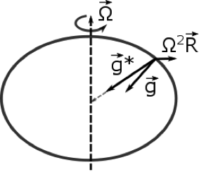
The resulting gravity that the Earth and everything on it feels is the vector sum of this real and this apparent force:

Since the centrifugal force depends on $\overrightarrow{R}$ , it is greatest at the equator and zero at the poles. As a result of the centrifugal force, the Earth has become slightly oblate, with an equatorial radius of 6378.1 km that is 0.34% greater than the polar radius of 6356.8 km. Note that $\overrightarrow{g}$[2]@5@5@+=faaagCart1ev2aaaKnaaaaWenf2ys9wBH5garuavP1wzZbItLDhis9wBH5garmWu51MyVXgaruWqVvNCPvMCG4uz3bqee0evGueE0jxyaibaieYlf9irVeeu0dXdh9vqqj=hHeeu0xXdbba9frFj0=OqFfea0dXdd9vqaq=JfrVkFHe9pgea0dXdar=Jb9hs0dXdbPYxe9vr0=vr0=vqpi0dc9GqpWqaaeaabiGaciaacaqabeaadaqaaqaaaOqaamaaFiaabaGaam4zaaGaay51Gaaaaa@356A@ is always perpendicular to Earth’s surface, which is very useful because the vertical coordinate is always chosen to be perpendicular to Earth's surface, so that $\overrightarrow{g}$[2]@5@5@+=faaagCart1ev2aaaKnaaaaWenf2ys9wBH5garuavP1wzZbItLDhis9wBH5garmWu51MyVXgaruWqVvNCPvMCG4uz3bqee0evGueE0jxyaibaieYlf9irVeeu0dXdh9vqqj=hHeeu0xXdbba9frFj0=OqFfea0dXdd9vqaq=JfrVkFHe9pgea0dXdar=Jb9hs0dXdbPYxe9vr0=vr0=vqpi0dc9GqpWqaaeaabiGaciaacaqabeaadaqaaqaaaOqaamaaFiaabaGaam4zaaGaay51Gaaaaa@356A@ is only in the z direction and, as the figure above indicates, does not point towards the center of the Earth (except at the poles and the equator). The value of g at the equator is 9.780 m s^–2, which is 0.052 m s^–2 smaller than the value of g at the poles, which is 9.832 m s^–2. The centrifugal force at the equator is Ω²R = (7.27 x 10^–5 s^–1)² (6.378 x 10⁶ m) = 0.033 m s^–2, and hence accounts for about 2/3 of the difference in g between the equator and the poles. The rest of the difference is due to the difference in g*, which is overestimated by the difference in equatorial and polar radii--the problem is more complicated than it might appear because Newton's law of gravitation only applies to point masses. At any rate, the difference between g at the poles and equator is small enough for a constant value of g = 9.8 m s^–2 to be suitable for most applications in atmospheric dynamics.

Combining Equations [10.14] and [10.15] yields a more useful form of the averaged momentum conservation in the rotating reference frame:

Coriolis Force

The Coriolis force, $-2\overrightarrow{\Omega }\times \overrightarrow{U}$, acts on an air parcel (or any other object) only when it is moving with respect to the Earth. It acts perpendicular to Earth's angular velocity vector and the air parcel's velocity vector. The explanation for the Coriolis force is usually broken into an explanation in the zonal (constant latitude) direction and the meridional (constant longitude) direction.

Zonal Flow (East–West Wind Velocity)

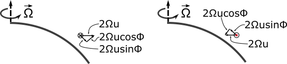
Consider an air parcel that is initially at rest and in hydrostatic balance but is impulsively accelerated to a velocity u to the east (see left side of figure below). Initially when it was at rest, it had the same acceleration as the Earth below it. However, after it accelerated to velocity u, it suddenly had more acceleration than it had before, throwing it out of hydrostatic balance. Look at the change in acceleration that comes from the air parcel suddenly acquiring a velocity to the east, which is just the acceleration after the velocity changes minus the acceleration before the velocity changes and equals (Ω+u/R)²R – Ω²R. To a very good approximation, this change equals the Coriolis force, 2Ωu. There is a vertical component that points up, but there is also a horizontal component of force that points to the right of the motion in the Northern Hemisphere and to the left in the Southern Hemisphere.

Now consider an air parcel that is initially at rest but is impulsively accelerated to a velocity u to the west (see right side of figure below). The air parcel suddenly has less angular momentum than it had before and experiences a decreased centrifugal force. This decrease in angular momentum, to a very good approximation, equals the Coriolis force, 2Ωu, but is pointed toward Earth's axis of rotation. There is a vertical component that points down, but the horizontal component of force that points to the right of the motion in the Northern Hemisphere and to the left in the Southern Hemisphere.

Coriolis force on an air parcel traveling zonally (left) to the east, where ⨂ indicates flow into the page, and (right) to the west, where the red dot in the circle indicates flow out of the page, for the Northern Hemisphere. The air parcel speed is u and the latitude is Φ.

Credit: W. Brune

We can write down the accelerations in the y and z directions due to the air moving to the east with speed u:

Meridional Flow (North–South Velocity)

What about an air parcel traveling to the north at a constant altitude? Note that the air parcel moving north starts at a greater distance from Earth’s axis and comes closer to Earth’s axis if it moves at the same height above the surface. Its angular momentum is conserved, so it is moving faster to the east than the Earth beneath it. As a result, it appears to move to the right or the east.

If the same air parcel moves to the south at the same height above Earth’s surface, then it moves to a greater distance from Earth’s rotation axis. Its angular momentum becomes less than that of Earth, it slows down relative to Earth, and it veers to the right of south or to the west.

In both the zonal and meridional flow cases, the air parcel's velocity with respect to the Earth causes the air parcel to have a different angular momentum from the Earth below it. Conservation of angular momentum during that motion requires that the apparent Coriolis force be added in order to describe the observed motion. See the video below (2:11) for further explanation:

Finding the Magnitude and Direction of the Coriolis Force

The magnitude of the horizontal Coriolis force is simply $2\Omega \left|\overrightarrow{V}\right|\sin \mathrm{\phi , }$where φ is the latitude. This magnitude applies to both the Northern and Southern Hemispheres. The direction of the Coriolis force is 90 degrees to the right of the horizontal velocity vector in the Northern Hemisphere and 90 degrees to the left of the horizontal velocity vector in the Southern Hemisphere.

10.4 Equations of Motion in Spherical Coordinates

The three variables used in spherical coordinates are:

• longitude (denoted by λ)
• latitude (denoted by φ)
• vertical distance (denoted by r from Earth’s center and by z from Earth’s surface, where z = r – a and a is Earth’s radius)

Conversion between spherical and Cartesian coordinates.

Credit: W. Brune

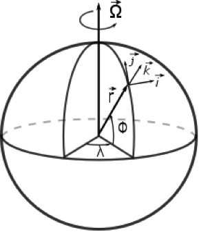
Note that the unit vectors in spherical coordinates change with position. For example, for an air parcel at the equator, the meridional unit vector, $\overrightarrow{j}$, is parallel to the Earth’s rotation axis, whereas for an air parcel near one of the poles, $\overrightarrow{j}$ is nearly perpendicular to the Earth’s rotation axis. In spherical coordinates, the velocity vector and its components are given by:

$$\begin{array}{l}\overrightarrow{U}=u\overrightarrow{i}+v\overrightarrow{j}+w\overrightarrow{k}\hfill \\ u=r\cos \varphi \frac{D\lambda }{Dt}\text{, }v=r\frac{D\varphi }{Dt}\text{, }w=\frac{Dz}{Dt}\hfill \end{array}$$[2]@5@5@+=faaahmart1ev3aaaKnaaaaWenf2ys9wBH5garuavP1wzZbItLDhis9wBH5garmWu51MyVXgaruWqVvNCPvMCaebbnrfifHhDYfgasaacH8srps0lbbf9q8WrFfeuY=ribbf9v8qqaqFr0xc9pk0xbba9q8WqFfea0=yr0RYxir=Jbba9q8aq0=yq=He9q8qqQ8frFve9Fve9Ff0dc9Gqpi0dmeaabaqaciGacaGaaeqabaWaaeaaeaaakeaafaWaaeGabaaabaaeeaaaaaaaaigBHn2Aa8qaceWGvbWdayaalaWdbiabg2da9iaadwhaceWGPbWdayaalaWdbiabgUcaRiaadAhaceWGQbWdayaalaWdbiabgUcaRiaadEhaceWGRbWdayaalaaabaWdbiaadwhacqGH9aqpcaWGYbGaci4yaiaac+gacaGGZbGaeqy1dy2aaSaaa8aabaWdbiaadseacqaH7oaBa8aabaWdbiaadseacaWG0baaaiaabYcacaqGGaGaaeiiaiaabccacaqGGaGaaeiiaiaabccacaWG2bGaeyypa0JaamOCamaalaaapaqaa8qacaWGebGaeqy1dygapaqaa8qacaWGebGaamiDaaaacaqGSaGaaeiiaiaabccacaqGGaGaaeiiaiaabccacaqGGaGaam4Daiabg2da9maalaaapaqaa8qacaWGebGaamOEaaWdaeaapeGaamiraiaadshaaaaaaaaa@6067@

$$\begin{array}{l}dx=r\cos \varphi d\lambda =\text{change in eastward distance}\cong a\cos \varphi d\lambda \hfill \\ dy=rd\varphi =\text{change in northward distance}\cong ad\varphi \hfill \\ dz=dr=\text{change in upward distance}\hfill \end{array}$$

Let’s now write the averaged momentum conservation equation [10.16] in component form in spherical coordinates. We will just show you how this conversion is done without actually taking you through all the steps. Note that we need to take the total derivatives of the unit vectors as well as the velocities:

$$\frac{D\overrightarrow{U}}{Dt}=\frac{D}{Dt}\left(\overrightarrow{i}u+\overrightarrow{j}v+\overrightarrow{k}w\right)=\overrightarrow{i}\frac{Du}{Dt}+u\frac{D\overrightarrow{i}}{Dt}+\overrightarrow{j}\frac{Dv}{Dt}+v\frac{D\overrightarrow{j}}{Dt}+\overrightarrow{k}\frac{Dw}{Dt}+w\frac{D\overrightarrow{k}}{Dt}$$

The terms containing derivatives of the unit vectors are called “metric terms.” They depend on the Earth being a sphere. In Cartesian coordinates, they equal zero.

Consider just one of these metric terms:

Since for any location, $\overrightarrow{j}$ is constant with time and $\overrightarrow{j}$ does not change as a function of altitude, that leaves $\overrightarrow{j}$[2]@5@5@+=faaagCart1ev2aqaKnaaaaWenf2ys9wBH5garuavP1wzZbItLDhis9wBH5garmWu51MyVXgaruWqVvNCPvMCG4uz3bqee0evGueE0jxyaibaieYlf9irVeeu0dXdh9vqqj=hHeeu0xXdbba9frFj0=OqFfea0dXdd9vqaq=JfrVkFHe9pgea0dXdar=Jb9hs0dXdbPYxe9vr0=vr0=vqpi0dc9GqpWqaaeaabiGaciaacaqabeaadaqaaqaaaOqaamaaFiaabaGaamOAaaGaay51Gaaaaa@356E@ dependent only on latitude and longitude.

Look at $\frac{\partial \overrightarrow{j}}{\partial y}$ first. Set y = 0 at the equator, and y = a (Earth’s radius) near the pole. As noted above, at the equator, $\overrightarrow{j}$ is parallel to Earth’s rotation axis, but near the pole, it is almost perpendicular to it. Thus the change in $\overrightarrow{j}$ going from south to north (increasing y) must be pointing down to Earth’s center and so $\overrightarrow{j}$ changes by $-\overrightarrow{k}$ times a small angular change while y changes by a times the same small angular change. The net result is that:

Using the same approach, we can show that:

The total derivatives of all three unit vectors are:

Putting this all together:

Similar analysis can be done for the other terms in the averaged momentum equation.

Coriolis force:

Gravity:

Pressure Gradient Force (PGF):

Turbulent friction (in the boundary layer only):

10.5 Are all the terms in these equations equally important? Let's use scale analysis.

Our equations of motion have several terms in them, and the question is, “Which ones are the largest and, thus, the most important?” The answer is, “It depends on the situation.” You can follow the following steps to determine which terms to keep and which you can safely ignore when you are trying to calculate the force balance for a specific atmospheric phenomenon. This process is called scale analysis and it can be applied to any conservation equation you would like to simplify.

1. Decide on the phenomenon of interest (e.g., cyclone, front, hurricane, tornado).
2. Determine the characteristic (i.e., typical) lengths and times over which the phenomenon occurs.
3. Determine the range of fluctuations of equation variables in space and time during the phenomenon.
4. Approximate derivatives (i.e., $\frac{\partial p}{\partial x}\sim \frac{\Delta p}{\Delta x}$[2]@5@5@+=faaagCart1ev2aqaKnaaaaWenf2ys9wBH5garuavP1wzZbItLDhis9wBH5garmWu51MyVXgaruWqVvNCPvMCG4uz3bqee0evGueE0jxyaibaieYlf9irVeeu0dXdh9vqqj=hHeeu0xXdbba9frFj0=OqFfea0dXdd9vqaq=JfrVkFHe9pgea0dXdar=Jb9hs0dXdbPYxe9vr0=vr0=vqpi0dc9GqpWqaaeaabiGaciaacaqabeaadaqaaqaaaOqaamaalaaabaGaeyOaIyRaamiCaaqaaiabgkGi2kaadIhaaaGaeSipIOZaaSaaaeaacqqHuoarcaWGWbaabaGaeuiLdqKaamiEaaaaaaa@3D90@ ).
5. Compare the magnitudes of the terms in the equation.
6. Keep only the relatively large terms (say, the top two orders of magnitude) and neglect the smaller terms.

The Coriolis Parameter

Define the Coriolis parameter as $f\equiv 2\Omega \sin \varphi$[2]@5@5@+=faaahmart1ev3aaaKnaaaaWenf2ys9wBH5garuavP1wzZbItLDhis9wBH5garmWu51MyVXgaruWqVvNCPvMCaebbnrfifHhDYfgasaacH8srps0lbbf9q8WrFfeuY=ribbf9v8qqaqFr0xc9pk0xbba9q8WqFfea0=yr0RYxir=Jbba9q8aq0=yq=He9q8qqQ8frFve9Fve9Ff0dc9Gqpi0dmeaabaqaciGacaGaaeqabaWaaeaaeaaakeaaqqaaaaaaaaGySf2yRbWdbiaadAgacqGHHjIUcaaIYaGaeuyQdCLaci4CaiaacMgacaGGUbGaeqy1dygaaa@3D3D@ . At 45^o N,  $f=\left(2\right)\left(7.27\times {10}^{-5}{\text{s}}^{-1}\right)\text{sin}{45}^{\text{o}}\sim {10}^{-4}{\text{s}}^{-1}$[2]@5@5@+=faaahmart1ev3aaaKnaaaaWenf2ys9wBH5garuavP1wzZbItLDhis9wBH5garmWu51MyVXgaruWqVvNCPvMCaebbnrfifHhDYfgasaacH8srps0lbbf9q8WrFfeuY=ribbf9v8qqaqFr0xc9pk0xbba9q8WqFfea0=yr0RYxir=Jbba9q8aq0=yq=He9q8qqQ8frFve9Fve9Ff0dc9Gqpi0dmeaabaqaciGacaGaaeqabaWaaeaaeaaakeaaqqaaaaaaaaGySf2yRbWdbiaadAgacqGH9aqpdaqadaWdaeaapeGaaGOmaaGaayjkaiaawMcaamaabmaapaqaa8qacaaI3aGaaiOlaiaaikdacaaI3aGaey41aqRaaGymaiaaicdapaWaaWbaaSqabeaapeGaeyOeI0IaaGynaaaakiaabohapaWaaWbaaSqabeaapeGaeyOeI0IaaGymaaaaaOGaayjkaiaawMcaaiaabohacaqGPbGaaeOBaiaaisdacaaI1aWdamaaCaaaleqabaWdbiaab+gaaaGccqWI8iIocaaIXaGaaGima8aadaahaaWcbeqaa8qacqGHsislcaaI0aaaaOGaae4Ca8aadaahaaWcbeqaa8qacqGHsislcaaIXaaaaaaa@522F@ . We will use this parameter in the scale analysis in the next section and then throughout the rest of the lesson.

10.6 Why do weather maps use pressure surfaces instead of height surfaces?

You can’t find a weather map of winds at 5000 m, but you can find one for 500 mb, which is about the same altitude as 5000 m (see figure below).

500 mb winds for 22 February 2015. Numbers are height above sea level in decameters (dam, tens of meters). For example, the height of the 500 mb surface in the high is 5940 m = 594 dam.

Credit: NOAA

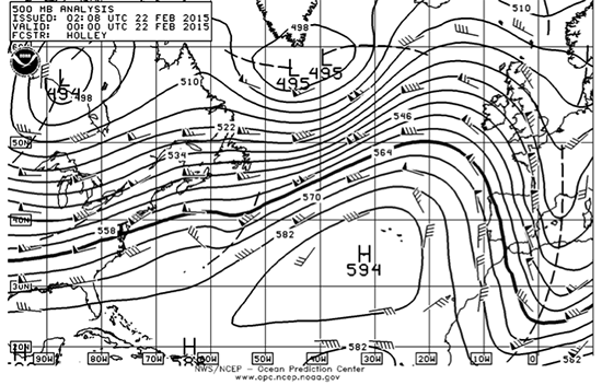
We will learn why weather maps use pressure as the vertical coordinate, but for now, we will show that higher altitudes on a constant-pressure surface correspond to higher pressures on an constant-altitude surface.

If we look down on the Earth, then we can plot the isobars as a function of latitude (y) and longitude (x). We can make a second plot of height surfaces on a constant-pressure surface (see figure below). Generally the pressure on average is greater at the equator on a given height surface than it is at the poles. This tilt makes sense if you think about the hydrostatic equilibrium equation because the temperature is greater at the equator than at the poles. Therefore, the scale height is greater, and so pressure decreases with height more gradually at the equator than it does at the poles.

A schematic of constant-pressure surfaces intersecting with constant-height surfaces from the pole to the equator.

Credit: W. Brune

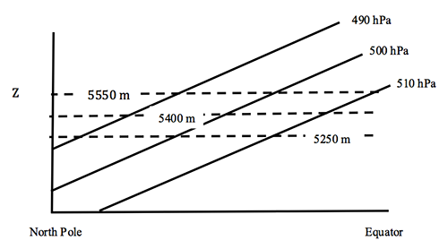
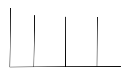
We can arbitrarily choose one height surface and see how the pressure changes as a function of latitude. We see that it increases from pole to equator (see figure below).

A schematic of isobars (constant pressure) on an x–y horizontal map at a constant height surface of 5400 m, as in the figure above.

Credit: W. Brune

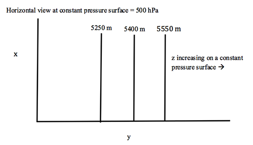
If we now arbitrarily choose a constant-pressure surface of, say, 500 mb, then the change in the height on an x–y horizontal plot on the pressure surface also shows an increase from pole to equator (see figure below).

A schematic of lines of constant height on an x–y horizontal map at a constant pressure surface of 500 hPa, as in the figure above.

Credit: W. Brune

Thus, low pressure on constant-height surfaces is related to low heights on constant-pressure surfaces. As a result of the hydrostatic approximation, for every height there is a unique pressure, so we can replace z with p as the vertical coordinate. We can then look at changes in variables as a function of x and y, but instead of doing this on a constant-height surface, we can do it on a constant-pressure surface.

We can now show how the equations of motion change when the vertical coordinate is switched from the height, z, to the pressure, p.

Consider first the pressure gradient force (PGF). The figure below provides a schematic of the math.

A cross section of pressure change on a x–z surface. Note that Δx, Δz, and Δp are all positive and Δp is the same in the horizontal and vertical.

Credit: W. Brune (after R. Najjar)

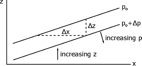
The slope of the isobar is just the change in z divided by the change in x on an isobar:

where the subscript “p” means “constant pressure.” Since Δp is the same in the vertical and the horizontal:

where the subscripts "x" and "z" mean constant eastward distance and constant height, respectively.

Multiplying both sides by 1/ρ and using the hydrostatic equilibrium equation:

Same for the y direction:

So, the geostrophic balance (Equation [10.24], [10.25]) in pressure coordinates becomes:

These equations can be rearranged to give the horizontal velocity on the pressure surface and can be rewritten as one in vector form:

where $\overrightarrow{V_g}$[2]@5@5@+=faaagCart1ev2aaaKnaaaaWenf2ys9wBH5garuavP1wzZbItLDhis9wBH5garmWu51MyVXgaruWqVvNCPvMCG4uz3bqee0evGueE0jxyaibaieYlf9irVeeu0dXdh9vqqj=hHeeu0xXdbba9frFj0=OqFfea0dXdd9vqaq=JfrVkFHe9pgea0dXdar=Jb9hs0dXdbPYxe9vr0=vr0=vqpi0dc9GqpWqaaeaabiGaciaacaqabeaadaqaaqaaaOqaamaaFiaabaGaamODamaaBaaaleaacaWGNbaabeaaaOGaay51Gaaaaa@369B@ is designated geostrophic velocity and ${\overrightarrow{\nabla }}_{p}z=\overrightarrow{i}\frac{\partial z}{\partial x}+\overrightarrow{j}\frac{\partial z}{\partial y}$[2]@5@5@+=faaagCart1ev2aaaKnaaaaWenf2ys9wBH5garuavP1wzZbItLDhis9wBH5garmWu51MyVXgaruWqVvNCPvMCG4uz3bqee0evGueE0jxyaibaieYlf9irVeeu0dXdh9vqqj=hHeeu0xXdbba9frFj0=OqFfea0dXdd9vqaq=JfrVkFHe9pgea0dXdar=Jb9hs0dXdbPYxe9vr0=vr0=vqpi0dc9GqpWqaaeaabiGaciaacaqabeaadaqaaqaaaOqaaabaaaaaaaaapeGafy4bIe9dayaalaWaaSbaaSqaa8qacaWGWbaapaqabaGcpeGaamOEaiabg2da9iqadMgapaGbaSaapeWaaSaaa8aabaWdbiabgkGi2kaadQhaa8aabaWdbiabgkGi2kaadIhaaaGaey4kaSIabmOAa8aagaWca8qadaWcaaWdaeaapeGaeyOaIyRaamOEaaWdaeaapeGaeyOaIyRaamyEaaaaaaa@453E@ is on a constant pressure surface.

Geopotential

We can write these equations a little differently by using the concept of geopotential. Geopotential, Φ, is the potential energy per unit mass of an air parcel at a height z, where zero potential energy is defined at the surface (z = 0).

In vector form, the velocities become:

Balance between Coriolis and pressure gradient forces and the resulting velocities of the wind in the Northern Hemisphere (NH) and Southern Hemisphere (SH).

Credit: W. Brune

A major advantage of using pressure coordinates is that the gradient of z or Φ is proportional to $\overrightarrow{V_g}$[2]@5@5@+=faaagCart1ev2aaaKnaaaaWenf2ys9wBH5garuavP1wzZbItLDhis9wBH5garmWu51MyVXgaruWqVvNCPvMCG4uz3bqee0evGueE0jxyaibaieYlf9irVeeu0dXdh9vqqj=hHeeu0xXdbba9frFj0=OqFfea0dXdd9vqaq=JfrVkFHe9pgea0dXdar=Jb9hs0dXdbPYxe9vr0=vr0=vqpi0dc9GqpWqaaeaabiGaciaacaqabeaadaqaaqaaaOqaamaaFiaabaGaamODamaaBaaaleaacaWGNbaabeaaaOGaay51Gaaaaa@369B@ for all pressure levels. This statement is not true for pressure gradients on height levels because you must know the density, ρ, as in Equations [10.24] and [10.25] [7], which varies dramatically with height.

The following video (1:19) provides a good overview of pressure surfaces:

10.7 Natural coordinates are better horizontal coordinates.

Understanding the results of a balance of forces can often be easier if we choose a horizontal coordinate system that is aligned naturally with the air flow, and not just set up in Cartesian coordinates x and y or spherical coordinates λ and φ. We can choose one direction—let’s call it s for streamline—so that it is aligned with the streamline (and is thus always parallel with the flow) and increases in the direction of the flow (i.e., downwind). The second direction—let’s call it n for normal—increases to the left of the flow. An interesting and noteworthy feature of natural coordinates is that the wind velocity is always positive because, by the definition of natural coordinates, the velocity vector is always pointed in the positive s direction.

For the horizontal momentum equation without friction:

$$\frac{D\overrightarrow{V}}{Dt}=-f\overrightarrow{k}\times \overrightarrow{V}-{\overrightarrow{\nabla }}_p\Phi$$

where $\overrightarrow{V}=\overrightarrow{i}u+\overrightarrow{j}v$ and ${\overrightarrow{\nabla }}_p$[2]@5@5@+=faaagCart1ev2aaaKnaaaaWenf2ys9wBH5garuavP1wzZbItLDhis9wBH5garmWu51MyVXgaruWqVvNCPvMCG4uz3bqee0evGueE0jxyaibaieYlf9irVeeu0dXdh9vqqj=hHeeu0xXdbba9frFj0=OqFfea0dXdd9vqaq=JfrVkFHe9pgea0dXdar=Jb9hs0dXdbPYxe9vr0=vr0=vqpi0dc9GqpWqaaeaabiGaciaacaqabeaadaqaaqaaaOqaamaaFiaabaGaey4bIenacaGLxdcadaWgaaWcbaGaamiCaaqabaaaaa@3725@ is the horizontal gradient operator on a pressure surface, not a height surface.

Let’s look at each term in the equation and put it in natural coordinates.

The acceleration of the air parcel: $$\frac{D\overrightarrow{V}}{Dt}$$

There are two ways that $\overrightarrow{V}$ can change. It can change by changing its speed ($V=\left|\overrightarrow{V}\right|$), $\frac{DV}{Dt}$ , which occurs in the streamline direction s, or by changing its direction, which occurs in the normal direction, n. Recall that n points to the left of the velocity vector.

Remember your physics, which showed that the acceleration due to rotation (the centripetal acceleration) is the velocity squared divided by the radius of curvature of the rotation. In this case, the rotation is the rotation of the air parcel as it moves horizontally over the Earth (not the rotation of the Earth itself). The acceleration is directed perpendicular to the motion and is directed towards the center of curvature. R is the radius of curvature of the changing direction, and by convention, R > 0 if the curvature is in the counterclockwise direction, and R < 0 if the curvature is in the clockwise direction. Hence the sign always works out if the centripetal acceleration is V²/R.

The Coriolis force:

$$-f\overrightarrow{k}\times \overrightarrow{V}$$[2]@5@5@+=faaagCart1ev2aaaKnaaaaWenf2ys9wBH5garuavP1wzZbItLDhis9wBH5garmWu51MyVXgaruWqVvNCPvMCG4uz3bqee0evGueE0jxyaibaieYlf9irVeeu0dXdh9vqqj=hHeeu0xXdbba9frFj0=OqFfea0dXdd9vqaq=JfrVkFHe9pgea0dXdar=Jb9hs0dXdbPYxe9vr0=vr0=vqpi0dc9GqpWqaaeaabiGaciaacaqabeaadaqaaqaaaOqaaiabgkHiTiaadAgacaaMc8+aa8HaaeaacaWGRbaacaGLxdcacqGHxdaTdaWhcaqaaiaadAhaaiaawEniamaaBaaaleaacaWGibaabeaaaaa@3E90@

The n component equals $-\mathrm{fV}$[2]@5@5@+=faaagCart1ev2aaaKnaaaaWenf2ys9wBH5garuavP1wzZbItLDhis9wBH5garmWu51MyVXgaruWqVvNCPvMCG4uz3bqee0evGueE0jxyaibaieYlf9irVeeu0dXdh9vqqj=hHeeu0xXdbba9frFj0=OqFfea0dXdd9vqaq=JfrVkFHe9pgea0dXdar=Jb9hs0dXdbPYxe9vr0=vr0=vqpi0dc9GqpWqaaeaabiGaciaacaqabeaadaqaaqaaaOqaaiabgkHiTiaadAgacaaMc8UaamODamaaBaaaleaacaWGibaabeaaaaa@3821@ because when f > 0, the force is to the right of the motion (i.e., streamline) and is, thus, negative because positive n points to the left of the motion. When f < 0, the force would be to the left in the positive n direction.

The pressure gradient force (PGF):

$$-{\overrightarrow{\nabla }}_p\Phi$$[2]@5@5@+=faaagCart1ev2aaaKnaaaaWenf2ys9wBH5garuavP1wzZbItLDhis9wBH5garmWu51MyVXgaruWqVvNCPvMCG4uz3bqee0evGueE0jxyaibaieYlf9irVeeu0dXdh9vqqj=hHeeu0xXdbba9frFj0=OqFfea0dXdd9vqaq=JfrVkFHe9pgea0dXdar=Jb9hs0dXdbPYxe9vr0=vr0=vqpi0dc9GqpWqaaeaabiGaciaacaqabeaadaqaaqaaaOqaaiabgkHiTmaaFiaabaGaey4bIenacaGLxdcadaWgaaWcbaGaamiCaaqabaGccqqHMoGraaa@3996@

The n component of $-{\overrightarrow{\nabla }}_p\Phi$[2]@5@5@+=faaagCart1ev2aaaKnaaaaWenf2ys9wBH5garuavP1wzZbItLDhis9wBH5garmWu51MyVXgaruWqVvNCPvMCG4uz3bqee0evGueE0jxyaibaieYlf9irVeeu0dXdh9vqqj=hHeeu0xXdbba9frFj0=OqFfea0dXdd9vqaq=JfrVkFHe9pgea0dXdar=Jb9hs0dXdbPYxe9vr0=vr0=vqpi0dc9GqpWqaaeaabiGaciaacaqabeaadaqaaqaaaOqaaiabgkHiTmaaFiaabaGaey4bIenacaGLxdcadaWgaaWcbaGaamiCaaqabaGccqqHMoGraaa@3996@ is just $-\frac{\partial \Phi }{\partial n}$[2]@5@5@+=faaagCart1ev2aqaKnaaaaWenf2ys9wBH5garuavP1wzZbItLDhis9wBH5garmWu51MyVXgaruWqVvNCPvMCG4uz3bqee0evGueE0jxyaibaieYlf9irVeeu0dXdh9vqqj=hHeeu0xXdbba9frFj0=OqFfea0dXdd9vqaq=JfrVkFHe9pgea0dXdar=Jb9hs0dXdbPYxe9vr0=vr0=vqpi0dc9GqpWqaaeaabiGaciaacaqabeaadaqaaqaaaOqaaiabgkHiTmaalaaabaGaeyOaIyRaeuOPdyeabaGaeyOaIyRaamOBaaaaaaa@3901@ .

Putting these pieces all together results in the equation for the n component of the horizontal momentum equation:

This equation is called the Gradient Wind Equation. The form of the equation in z coordinates is sometimes useful:

Keep in mind that V is always positive in Equations [10.34] because they are cast in natural coordinates.

Let’s rearrange Equation [10.34a] slightly by moving the centripetal acceleration over to the right hand side, where it represents a centrifugal force. Then, by considering which of the terms are the most important, we can apply this equation to different situations:

We can use the Rossby number to help determine which of the above balances dominates. The Rossby number is defined to be the magnitude of the acceleration divided by the magnitude of the Coriolis force. When applied to the gradient wind equation, the Rossby number is given by

If R_o << 1, then the centrifugal force is much smaller than the Coriolis force and the Coriolis force must balance the PGF (geostrophic balance).

If R_o >> 1, then the Coriolis force is much smaller than the centrifugal force and the centrifugal force must balance the PGF (cyclostrophic balance).

If R_o ~ 1, then the Coriolis force and the centrifugal force balance each other (inertial balance).

10.8 A Closer Look at the Four Force Balances

Geostrophic Balance

This balance occurs often in atmospheric flow that is a straight line (R = ±∞) well above Earth’s surface, so that friction does not matter. The Rossby number, R_o, is much less than 1.

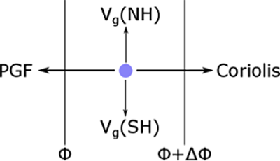
Let’s think about how this balance might occur. Assume that an air parcel is placed in the midst of a fixed horizontal pressure gradient in the Northern Hemisphere and is initially at rest ($\overrightarrow{V}=0$[2]@5@5@+=faaagCart1ev2aaaKnaaaaWenf2ys9wBH5garuavP1wzZbItLDhis9wBH5garmWu51MyVXgaruWqVvNCPvMCG4uz3bqee0evGueE0jxyaibaieYlf9irVeeu0dXdh9vqqj=hHeeu0xXdbba9frFj0=OqFfea0dXdd9vqaq=JfrVkFHe9pgea0dXdar=Jb9hs0dXdbPYxe9vr0=vr0=vqpi0dc9GqpWqaaeaabiGaciaacaqabeaadaqaaqaaaOqaamaaFiaabaGaamOvaaGaay51GaGaeyypa0JaaGimaaaa@3719@), as shown in the figure below. The Coriolis force is thus zero and the parcel begins to move from high pressure toward low pressure. However, as the parcel accelerates and attains a velocity parallel to the pressure gradient, the Coriolis force develops perpendicular and to the right of the velocity vector and the PGF. The resulting acceleration is now the vector sum of the PGF and the Coriolis force and turns the parcel to the right. As the velocity continues to increase, the Coriolis force increases but always stays perpendicular and to the right of the velocity vector while the PGF always stays parallel to the pressure gradient. Eventually, the PGF and Coriolis force become equal and opposite and the air parcel will move perpendicular to the horizontal pressure gradient. This condition is called geostrophic balance. We have simplified somewhat the approach to geostrophic equilibrium because, in reality, air parcels would overshoot and undergo inertial oscillations (discussed below) and because the pressure field would evolve in response to the motion.

How geostrophic balance is achieved for an air parcel starting at rest. The PGF is always there, but the Coriolis force is zero until the air parcel acquires some velocity. In the figure, v_g is used to represent the geostrophic velocity.

Credit: H.N. Shirer

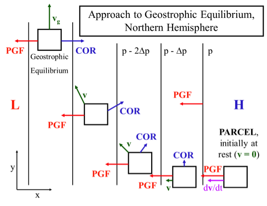
Let the Coriolis force per unit mass be designated as $Co=-f{V}_{}$[2]@5@5@+=faaagCart1ev2aaaKnaaaaWenf2ys9wBH5garuavP1wzZbItLDhis9wBH5garmWu51MyVXgaruWqVvNCPvMCG4uz3bqee0evGueE0jxyaibaieYlf9irVeeu0dXdh9vqqj=hHeeu0xXdbba9frFj0=OqFfea0dXdd9vqaq=JfrVkFHe9pgea0dXdar=Jb9hs0dXdbPYxe9vr0=vr0=vqpi0dc9GqpWqaaeaabiGaciaacaqabeaadaqaaqaaaOqaaiaadoeacaWGVbGaeyypa0JaeyOeI0IaamOzaiaadAhadaWgaaWcbaGaamisaaqabaaaaa@3958@ and the pressure gradient force per unit mass as $P=-\frac{\partial \Phi }{\partial n}$[2]@5@5@+=faaagCart1ev2aaaKnaaaaWenf2ys9wBH5garuavP1wzZbItLDhis9wBH5garmWu51MyVXgaruWqVvNCPvMCG4uz3bqee0evGueE0jxyaibaieYlf9irVeeu0dXdh9vqqj=hHeeu0xXdbba9frFj0=OqFfea0dXdd9vqaq=JfrVkFHe9pgea0dXdar=Jb9hs0dXdbPYxe9vr0=vr0=vqpi0dc9GqpWqaaeaabiGaciaacaqabeaadaqaaqaaaOqaaiaadcfacqGH9aqpcqGHsisldaWcaaqaaiabgkGi2kabfA6agbqaaiabgkGi2kaad6gaaaaaaa@3ADB@ . Then the force balances are shown in the figure below.

Geostrophic force balance in (a) the Northern Hemisphere and (b) the Southern Hemisphere shown in natural coordinates. Note that the n direction is always to the left of the velocity when looking downwind. In the figure, V_g is used to represent the geostrophic velocity.

Credit: W. Brune (after R. Najjar and An Introduction to Dynamic Meteorology, Fifth Edition, J. R. Holton and G. J. Hakim, 2013)

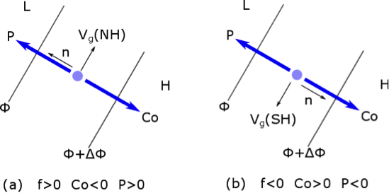
Note that the Coriolis force is always to the right of the velocity vector in the Northern Hemisphere. It is always to the left of the velocity vector in the Southern Hemisphere. When the pressure gradient force and Coriolis force are in balance, the PGF is to the left of the velocity vector and the Coriolis force is to the right in the Northern Hemisphere. Watch the video below (1:10) for further explanation:

Inertial Balance

In this case, the pressure gradient force is minimal and the centrifugal and Coriolis forces are in balance.

Let the centrifugal force be designated by $Ce=-\frac{V{}^2}{R}$[2]@5@5@+=faaagCart1ev2aaaKnaaaaWenf2ys9wBH5garuavP1wzZbItLDhis9wBH5garmWu51MyVXgaruWqVvNCPvMCG4uz3bqee0evGueE0jxyaibaieYlf9irVeeu0dXdh9vqqj=hHeeu0xXdbba9frFj0=OqFfea0dXdd9vqaq=JfrVkFHe9pgea0dXdar=Jb9hs0dXdbPYxe9vr0=vr0=vqpi0dc9GqpWqaaeaabiGaciaacaqabeaadaqaaqaaaOqaaiaadoeacaWGLbGaeyypa0JaeyOeI0YaaSaaaeaacaWG2bWaaSbaaSqaaiaadIeaaeqaaOWaaWbaaSqabeaacaaIYaaaaaGcbaGaamOuaaaaaaa@3A47@ .

Inertial balance in (a) the Northern Hemisphere and (b) the Southern Hemisphere shown in natural coordinates. Note that the n direction is always to the left of the velocity when looking downwind.

Credit: W. Brune (after R. Najjar)

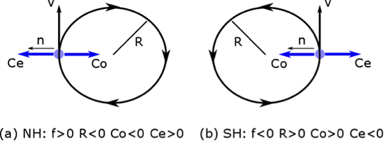
We can manipulate Equation [10.37] to find the radius of the circle:

For f = 10^–4 s^–1 and V = 10 m s^–1, R = –100 km. Inertial balance is not a major balance in the atmosphere because there is almost always a significant pressure gradient, but it can be important in oceans.

Cyclostrophic Balance

The balance in this case is between the pressure gradient force and the centrifugal force.

Cyclostrophic balance for (a) cyclonic flow and (b) anticyclonic flow in the Northern Hemisphere shown in natural coordinates. Note that the n direction is always to the left of the velocity when looking downwind. In the Southern Hemisphere, (b) is cyclonic and (a) is anticyclonic.

Credit: W. Brune (after R. Najjar and An Introduction to Dynamic Meteorology, Fifth Edition, J. R. Holton and G. J. Hakim, 2013)

In this case, the scale of the motion is so small that Coriolis acceleration is not important. The Rossby number, R_o = centrifugal acceleration / Coriolis >> 1.

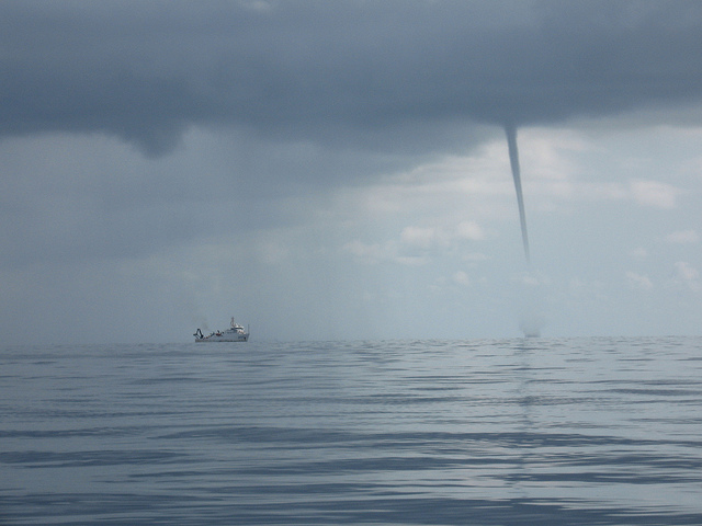
Examples of motion in cyclostrophic balance are tornadoes, dust devils, water spouts, and other small atmospheric circulations, such as the vortex you sometimes see when leaves get swept off the ground. These can be either cyclonic or anticyclonic and, in fact, a few percent of tornadoes in the Northern Hemisphere are anticyclonic. Another common example of cyclostrophic balance is the vortex seen when a bathtub or sink is draining.

NOAA Ship NANCY FOSTER dwarfed by waterspout. Gulf of Mexico. Summer, 2007.

Credit: NOAA Photo Library [8] via flickr

Gradient Balance

In gradient balance, the pressure gradient force, Coriolis force, and horizontal centrifugal force are all important. This balance occurs as wind in a pressure gradient field goes around a curve. There are many examples of this type of flow on any weather map—any synoptic-scale pressure gradient for which the isobars curve is an example of gradient flow.

To solve this equation for velocity, we can use the quadratic equation:

$\frac{f^2{R}^2}{4}$[2]@5@5@+=faaagCart1ev2aaaKnaaaaWenf2ys9wBH5garuavP1wzZbItLDhis9wBH5garmWu51MyVXgaruWqVvNCPvMCG4uz3bqee0evGueE0jxyaibaieYlf9irVeeu0dXdh9vqqj=hHeeu0xXdbba9frFj0=OqFfea0dXdd9vqaq=JfrVkFHe9pgea0dXdar=Jb9hs0dXdbPYxe9vr0=vr0=vqpi0dc9GqpWqaaeaabiGaciaacaqabeaadaqaaqaaaOqaamaalaaabaGaamOzamaaCaaaleqabaGaaGOmaaaakiaadkfadaahaaWcbeqaaiaaikdaaaaakeaacaaI0aaaaaaa@3740@       is always positive, so, for a given hemisphere (say, the Northern Hemisphere) there are eight possibilities because R can be either positive or negative, $\frac{\partial \Phi }{\partial n}$[2]@5@5@+=faaagCart1ev2aaaKnaaaaWenf2ys9wBH5garuavP1wzZbItLDhis9wBH5garmWu51MyVXgaruWqVvNCPvMCG4uz3bqee0evGueE0jxyaibaieYlf9irVeeu0dXdh9vqqj=hHeeu0xXdbba9frFj0=OqFfea0dXdd9vqaq=JfrVkFHe9pgea0dXdar=Jb9hs0dXdbPYxe9vr0=vr0=vqpi0dc9GqpWqaaeaabiGaciaacaqabeaadaqaaqaaaOqaamaalaaabaGaeyOaIyRaeuOPdyeabaGaeyOaIyRaamOBaaaaaaa@3813@   can be positive or negative, and we have the ± sign in between the two terms on the right-hand side of Equation [10.40].

The table above gives the results for the Northern Hemisphere (f > 0). We are looking for whether positive or negative values of R and $\frac{\partial \Phi }{\partial n}$[2]@5@5@+=faaagCart1ev2aaaKnaaaaWenf2ys9wBH5garuavP1wzZbItLDhis9wBH5garmWu51MyVXgaruWqVvNCPvMCG4uz3bqee0evGueE0jxyaibaieYlf9irVeeu0dXdh9vqqj=hHeeu0xXdbba9frFj0=OqFfea0dXdd9vqaq=JfrVkFHe9pgea0dXdar=Jb9hs0dXdbPYxe9vr0=vr0=vqpi0dc9GqpWqaaeaabiGaciaacaqabeaadaqaaqaaaOqaamaalaaabaGaeyOaIyRaeuOPdyeabaGaeyOaIyRaamOBaaaaaaa@3813@   give non-negative and real values for V because only non-negative and real values for V are physically possible. The reason why real negative values of V are not possible is because the gradient wind balance has been written down in natural coordinates.

For R > 0 and $\frac{\partial \Phi }{\partial n}$[2]@5@5@+=faaagCart1ev2aaaKnaaaaWenf2ys9wBH5garuavP1wzZbItLDhis9wBH5garmWu51MyVXgaruWqVvNCPvMCG4uz3bqee0evGueE0jxyaibaieYlf9irVeeu0dXdh9vqqj=hHeeu0xXdbba9frFj0=OqFfea0dXdd9vqaq=JfrVkFHe9pgea0dXdar=Jb9hs0dXdbPYxe9vr0=vr0=vqpi0dc9GqpWqaaeaabiGaciaacaqabeaadaqaaqaaaOqaamaalaaabaGaeyOaIyRaeuOPdyeabaGaeyOaIyRaamOBaaaaaaa@3813@    > 0, V is always negative, so there are no physical solutions.

For R > 0 and $\frac{\partial \Phi }{\partial n}$[2]@5@5@+=faaagCart1ev2aaaKnaaaaWenf2ys9wBH5garuavP1wzZbItLDhis9wBH5garmWu51MyVXgaruWqVvNCPvMCG4uz3bqee0evGueE0jxyaibaieYlf9irVeeu0dXdh9vqqj=hHeeu0xXdbba9frFj0=OqFfea0dXdd9vqaq=JfrVkFHe9pgea0dXdar=Jb9hs0dXdbPYxe9vr0=vr0=vqpi0dc9GqpWqaaeaabiGaciaacaqabeaadaqaaqaaaOqaamaalaaabaGaeyOaIyRaeuOPdyeabaGaeyOaIyRaamOBaaaaaaa@3813@   < 0, only the plus sign gives a positive V and thus a physical solution.

For R < 0 and $\frac{\partial \Phi }{\partial n}$[2]@5@5@+=faaagCart1ev2aaaKnaaaaWenf2ys9wBH5garuavP1wzZbItLDhis9wBH5garmWu51MyVXgaruWqVvNCPvMCG4uz3bqee0evGueE0jxyaibaieYlf9irVeeu0dXdh9vqqj=hHeeu0xXdbba9frFj0=OqFfea0dXdd9vqaq=JfrVkFHe9pgea0dXdar=Jb9hs0dXdbPYxe9vr0=vr0=vqpi0dc9GqpWqaaeaabiGaciaacaqabeaadaqaaqaaaOqaamaalaaabaGaeyOaIyRaeuOPdyeabaGaeyOaIyRaamOBaaaaaaa@3813@   > 0, only the plus sign gives a positive V and thus a physical solution.

For R < 0 and $\frac{\partial \Phi }{\partial n}$[2]@5@5@+=faaagCart1ev2aaaKnaaaaWenf2ys9wBH5garuavP1wzZbItLDhis9wBH5garmWu51MyVXgaruWqVvNCPvMCG4uz3bqee0evGueE0jxyaibaieYlf9irVeeu0dXdh9vqqj=hHeeu0xXdbba9frFj0=OqFfea0dXdd9vqaq=JfrVkFHe9pgea0dXdar=Jb9hs0dXdbPYxe9vr0=vr0=vqpi0dc9GqpWqaaeaabiGaciaacaqabeaadaqaaqaaaOqaamaalaaabaGaeyOaIyRaeuOPdyeabaGaeyOaIyRaamOBaaaaaaa@3813@   < 0, both roots give positive V and thus physical solutions.

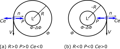
So there are four physical solutions. However, there is one more constraint. This additional constraint is that the absolute angular momentum about the axis of rotation at the latitude of the air parcel should be positive in the Northern Hemisphere (and negative in the Southern Hemisphere). Without proof, we state that only two of the four physically possible cases meet this criterion of positive absolute angular momentum in the Northern Hemisphere. They are:

1. Regular low: R > 0 and $\frac{\partial \Phi }{\partial n}$[2]@5@5@+=faaagCart1ev2aaaKnaaaaWenf2ys9wBH5garuavP1wzZbItLDhis9wBH5garmWu51MyVXgaruWqVvNCPvMCG4uz3bqee0evGueE0jxyaibaieYlf9irVeeu0dXdh9vqqj=hHeeu0xXdbba9frFj0=OqFfea0dXdd9vqaq=JfrVkFHe9pgea0dXdar=Jb9hs0dXdbPYxe9vr0=vr0=vqpi0dc9GqpWqaaeaabiGaciaacaqabeaadaqaaqaaaOqaamaalaaabaGaeyOaIyRaeuOPdyeabaGaeyOaIyRaamOBaaaaaaa@3813@  < 0 and $V_{}=-\frac{fR}{2}+\sqrt{\frac{f^2{R}^2}{4}-R\frac{\partial \Phi }{\partial n}}$[2]@5@5@+=faaagCart1ev2aaaKnaaaaWenf2ys9wBH5garuavP1wzZbItLDhis9wBH5garmWu51MyVXgaruWqVvNCPvMCG4uz3bqee0evGueE0jxyaibaieYlf9irVeeu0dXdh9vqqj=hHeeu0xXdbba9frFj0=OqFfea0dXdd9vqaq=JfrVkFHe9pgea0dXdar=Jb9hs0dXdbPYxe9vr0=vr0=vqpi0dc9GqpWqaaeaabiGaciaacaqabeaadaqaaqaaaOqaaiaadAhadaWgaaWcbaGaamisaaqabaGccqGH9aqpcqGHsisldaWcaaqaaiaadAgacaaMi8UaamOuaaqaaiaaikdaaaGaey4kaSYaaOaaaeaadaWcaaqaaiaadAgadaahaaWcbeqaaiaaikdaaaGccaWGsbWaaWbaaSqabeaacaaIYaaaaaGcbaGaaGinaaaacqGHsislcaWGsbWaaSaaaeaacqGHciITcqqHMoGraeaacqGHciITcaWGUbaaaaWcbeaaaaa@475A@
2. Regular high: R < 0 and $\frac{\partial \Phi }{\partial n}$[2]@5@5@+=faaagCart1ev2aaaKnaaaaWenf2ys9wBH5garuavP1wzZbItLDhis9wBH5garmWu51MyVXgaruWqVvNCPvMCG4uz3bqee0evGueE0jxyaibaieYlf9irVeeu0dXdh9vqqj=hHeeu0xXdbba9frFj0=OqFfea0dXdd9vqaq=JfrVkFHe9pgea0dXdar=Jb9hs0dXdbPYxe9vr0=vr0=vqpi0dc9GqpWqaaeaabiGaciaacaqabeaadaqaaqaaaOqaamaalaaabaGaeyOaIyRaeuOPdyeabaGaeyOaIyRaamOBaaaaaaa@3813@  < 0 and $V_{}=-\frac{fR}{2}-\sqrt{\frac{f^2{R}^2}{4}-R\frac{\partial \Phi }{\partial n}}$[2]@5@5@+=faaagCart1ev2aaaKnaaaaWenf2ys9wBH5garuavP1wzZbItLDhis9wBH5garmWu51MyVXgaruWqVvNCPvMCG4uz3bqee0evGueE0jxyaibaieYlf9irVeeu0dXdh9vqqj=hHeeu0xXdbba9frFj0=OqFfea0dXdd9vqaq=JfrVkFHe9pgea0dXdar=Jb9hs0dXdbPYxe9vr0=vr0=vqpi0dc9GqpWqaaeaabiGaciaacaqabeaadaqaaqaaaOqaaiaadAhadaWgaaWcbaGaamisaaqabaGccqGH9aqpcqGHsisldaWcaaqaaiaadAgacaaMi8UaamOuaaqaaiaaikdaaaGaeyOeI0YaaOaaaeaadaWcaaqaaiaadAgadaahaaWcbeqaaiaaikdaaaGccaWGsbWaaWbaaSqabeaacaaIYaaaaaGcbaGaaGinaaaacqGHsislcaWGsbWaaSaaaeaacqGHciITcqqHMoGraeaacqGHciITcaWGUbaaaaWcbeaaaaa@4765@

These two cases are depicted in the second and third panels of the figure below.

Gradient balance in Northern Hemisphere. left: Geostrophic balance; center: regular low balance; right: regular high balance. Note that the PGF is independent of velocity but both the Coriolis force and the centrifugal force are dependent on velocity. In the figure, v_g is used to represent the geostrophic velocity (only the PGF and Coriolis force are important) and v_gr is used to represent the gradient wind velocity (the PGF, Coriolis force, and centrifugal force are all important).

Credit: H.N. Shirer

The video below ( 3:22) explains these four force balances in more detail:

10.9 See how the gradient wind has a role in weather.

Note that the wind speed for gradient flow differs from the wind speed of geostrophic flow. Let’s see why. Start with the geostrophic balance (Equation [10.36]) and rearrange the equation to get an expression for the geostrophic wind speed:

Replacing the pressure gradient force ($\frac{\partial \Phi }{\partial n}$[2]@5@5@+=faaagCart1ev2aaaKnaaaaWenf2ys9wBH5garuavP1wzZbItLDhis9wBH5garmWu51MyVXgaruWqVvNCPvMCG4uz3bqee0evGueE0jxyaibaieYlf9irVeeu0dXdh9vqqj=hHeeu0xXdbba9frFj0=OqFfea0dXdd9vqaq=JfrVkFHe9pgea0dXdar=Jb9hs0dXdbPYxe9vr0=vr0=vqpi0dc9GqpWqaaeaabiGaciaacaqabeaadaqaaqaaaOqaamaalaaabaGaeyOaIyRaeuOPdyeabaGaeyOaIyRaamOBaaaaaaa@3813@ ) with –fV_g in the gradient balance equation results in an equation that relates these gradient velocities to the geostrophic velocity:

In a regular low (middle, figure below), R > 0 so that V_g > V. The velocity in a curve around a low-pressure area is subgeostrophic.

In a regular high (right, figure below), R < 0 so that V_g < V. The velocity in a curve around a high-pressure area is supergeostrophic.

Gradient balance in Northern Hemisphere. left: Geostrophic balance; center: regular low balance; right: regular high balance. Note that the PGF is independent of velocity but both the Coriolis force and the centrifugal acceleration are dependent on velocity. In the figure the geostrophic velocity is represented by v_g and the gradient wind velocity is represented by v_gr.

Click here for an accessible alternative to the figure above

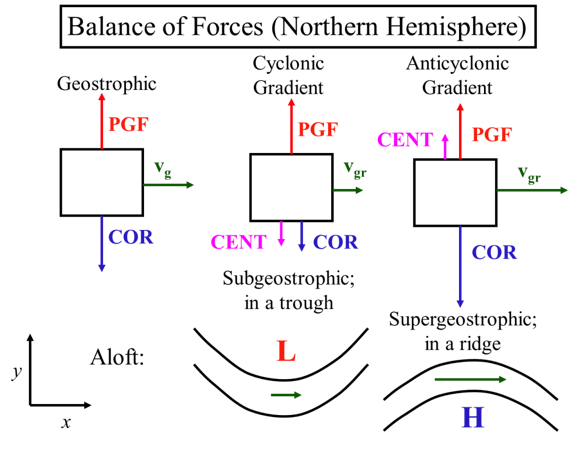
Balance of Forces (Northern Hemisphere)

*Represented as boxes with arrows*

Geostrophic:

PGF arrow pointing up, COR arrow pointing down (about the same size as PGF), v_g arrow pointing right

Subgeostrophic in a trough: Low pressure in a trough with a green arrow underneath pointing right

Supergeostrophic; in a ridge: high pressure below a hill with a green arrow above pointing right

Cyclonic Gradient:

PGF up, COR down (smaller than PGF), CENT down (smaller than COR), v_gr right (smaller than geostrophic v_g)

Anticyclonic Gradient:

PGF up, CENT up (smaller than PGF), COR down (larger than PGF), v_gr ( larger than geostrophic v_g)

Credit: H.N. Shirer

Think of it this way. The pressure gradient force is independent of velocity and so is always there for a given geopotential gradient. In a regular low, the centrifugal and Coriolis forces, both dependent on velocity, sum together to equal the pressure gradient force, whereas for geostrophic flow, only the Coriolis force does. Thus, the velocity in the gradient balance case must be less than the geostrophic velocity for the same geopotential gradient.

So how do subgeostrophic and supergeostrophic flow affect weather?

Supergeostrophic flow around ridges and subgeostrophic flow around troughs helps to explain the convergence and divergence patterns aloft that are linked to vertical motions.

Look at the figure below, starting on the left. Going from geostrophic flow in the straight section to supergeostrophic flow at the ridge’s peak causes divergence aloft. This divergence causes an upward vertical velocity, which causes a low pressure area and convergence at the surface. As the air rounds the ridge’s peak, it slows down to become geostrophic, and then continues to slow down even more as the flow becomes subgeostrophic around the trough, thus causing convergence aloft. This convergence aloft causes a downward velocity, which causes high pressure and divergence at the surface.

Subgeostrophic and supergeostrophic velocities in flow aloft in the Northern Hemisphere.

Click here for an accessible alternative to the figure above

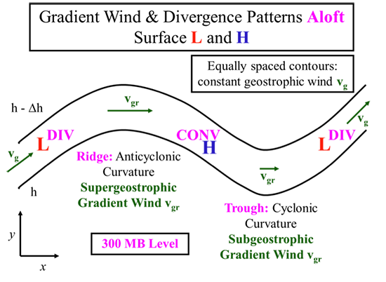
Gradient Wing & Divergence Patterns Aloft, Surface Low and High Pressure

Diagram of a wave shape. It starts as a low-pressure zone with a constant geostrophic wind (v_g) moving up along the wave, it is also labeled with divergence, at the ridge of the wave super geostrophic gradient wind v_gr is horizontal. The ridge also has anticyclonic curvature. The wave then moves downward, in a high-pressure zone, labeled with convergence until it reaches a trough with cyclonic curvature and subgeostropic gradient wing v_gr which is represented by a horizontal arrow. The wave then repeats and v_g goes upward toward the ridge from a low-pressure zone that is diverging.

Credit: H.N. Shirer

So downwind of a trough is the favored location for divergence aloft, upward motion, and a surface low [9]. Downwind of a ridge is the favored location for convergence aloft, downward motion, and a surface high. Since ridges form around high pressure aloft and troughs form around low pressure aloft, we see that the high aloft is offset relative to the surface low and the low aloft is offset relative to the surface high.

Thus subgeostrophic flow and supergeostrophic flow aloft are directly related to the formation of weather at the surface. Other factors like vorticity are also very important. The video below (1:09) describes how the gradient wind flow aloft can affect surface weather.

10.10 What does turbulent drag do to horizontal boundary layer flow?

The turbulent drag force on the horizontal air flow within the atmospheric boundary layer can approach the size of the other terms in the horizontal equation of motion. Note that this turbulent drag force acts to reduce the air velocity and therefore is opposite the air flow velocity vector. 

Let’s look at the force balance when the turbulent drag force is included. We will call this turbulent drag "friction" because it is commonly called that, but it is really quite different.

Horizontal map showing the geostrophic wind with friction in the Northern Hemisphere.

Credit: W. Brune

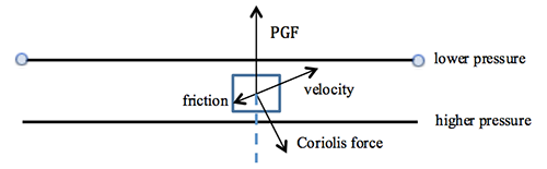
Note that the turbulent drag (friction) force is parallel to the velocity vector and is opposite in direction.

In the x-direction (along the isobars) the balance of forces is:

friction (x-component) = Coriolis (x-component).

In the y-direction (perpendicular to the isobars), the balance of opposing forces is:

friction (y-component) + Coriolis (y-component) = PGF

Because of the turbulent drag force and the velocity dependence of the Coriolis force, the parcel velocity points toward the lower pressure and the air parcel will tend to move across isobars toward the low pressure. Typical cross-isobaric flow in the boundary layer makes an angle of 30^o with the isobars. Thus, surface air moves toward low pressure and away from high pressure.

Above the atmospheric boundary layer, however, turbulent drag is not generally important and geostrophic and gradient flows are good approximations.

The effects of turbulent drag are very important for weather. When divergence aloft causes upward-moving air below, it becomes associated with a low-pressure region near Earth's surface. A pressure gradient force is created, but the air moving toward the low pressure is turned to travel counterclockwise around the low by the Coriolis force. However, turbulent drag slows the wind and turns it to cross isobars toward the low pressure, creating convergence, which causes uplift, clouds, and perhaps precipitation. The opposite is true for surface high-pressure regions occurring under regions of convergence aloft, which causes descent. The anticyclonic winds around the surface high are slowed and turn outward, causing divergence near the surface, leading to descending air and clear skies. The following video (1:43) provides further discussion of friction:

10.11 Why are midlatitude winds mostly westerly (i.e., eastward)?

The answer seems simple. More solar energy is deposited in the tropics than near the poles and as a result, the air is warmer in the tropics than the poles, where there is net radiative cooling. According to the hydrostatic equilibrium equation, the fall-off in pressure with altitude is less in the tropics than at higher latitudes, and as a result, for any height surface, the pressure is greater in the tropics than near the poles, setting up a pressure gradient force on each height surface that drives the wind poleward. As the air moves poleward, atmospheric processes such as the Coriolis force, which we saw occurs because of conservation of angular momentum, and synoptic-scale disturbances at higher latitudes cause the air to veer to the right in the Northern Hemisphere and to the left in the Southern Hemisphere.

Thermal Wind

With this broad concept in mind, we can consider the idea of the thermal wind, which is not really a wind, but instead is a difference in winds at two heights. We will see that the thermal wind is proportional to the horizontal temperature gradient. To show this relationship mathematically, we start with the geostrophic balance equation and apply the Ideal Gas Law and the hydrostatic equilibrium equation.

Look at the x and y components of Equation [10.33] for geostrophic winds:

Use the hydrostatic equation and the Ideal Gas Law to relate T to $\Phi$[2]@5@5@+=faaagCart1ev2aaaKnaaaaWenf2ys9wBH5garuavP1wzZbItLDhis9wBH5garmWu51MyVXgaruWqVvNCPvMCG4uz3bqee0evGueE0jxyaibaieYlf9irVeeu0dXdh9vqqj=hHeeu0xXdbba9frFj0=OqFfea0dXdd9vqaq=JfrVkFHe9pgea0dXdar=Jb9hs0dXdbPYxe9vr0=vr0=vqpi0dc9GqpWqaaeaabiGaciaacaqabeaadaqaaqaaaOqaaiabfA6agbaa@3444@ :

Take $\frac{\partial }{\partial p}$[2]@5@5@+=faaagCart1ev2aqaKnaaaaWenf2ys9wBH5garuavP1wzZbItLDhis9wBH5garmWu51MyVXgaruWqVvNCPvMCG4uz3bqee0evGueE0jxyaibaieYlf9irVeeu0dXdh9vqqj=hHeeu0xXdbba9frFj0=OqFfea0dXdd9vqaq=JfrVkFHe9pgea0dXdar=Jb9hs0dXdbPYxe9vr0=vr0=vqpi0dc9GqpWqaaeaabiGaciaacaqabeaadaqaaqaaaOqaamaalaaabaGaeyOaIylabaGaeyOaIyRaamiCaaaaaaa@369C@ of equations in [10.41], starting with the equation for $v_g$[2]@5@5@+=faaagCart1ev2aaaKnaaaaWenf2ys9wBH5garuavP1wzZbItLDhis9wBH5garmWu51MyVXgaruWqVvNCPvMCG4uz3bqee0evGueE0jxyaibaieYlf9irVeeu0dXdh9vqqj=hHeeu0xXdbba9frFj0=OqFfea0dXdd9vqaq=JfrVkFHe9pgea0dXdar=Jb9hs0dXdbPYxe9vr0=vr0=vqpi0dc9GqpWqaaeaabiGaciaacaqabeaadaqaaqaaaOqaaiaadAhadaWgaaWcbaGaam4zaaqabaaaaa@34DD@ :

Taking the same approach with the equation for $u_g$[2]@5@5@+=faaagCart1ev2aaaKnaaaaWenf2ys9wBH5garuavP1wzZbItLDhis9wBH5garmWu51MyVXgaruWqVvNCPvMCG4uz3bqee0evGueE0jxyaibaieYlf9irVeeu0dXdh9vqqj=hHeeu0xXdbba9frFj0=OqFfea0dXdd9vqaq=JfrVkFHe9pgea0dXdar=Jb9hs0dXdbPYxe9vr0=vr0=vqpi0dc9GqpWqaaeaabiGaciaacaqabeaadaqaaqaaaOqaaiaadwhadaWgaaWcbaGaam4zaaqabaaaaa@34DC@ gives the Thermal Wind Equations:

These equations are very powerful because they reveal that measurements of temperature only (which are relatively easy to make) make it possible to determine the changes in the horizontal wind with height, assuming that the geostrophic and hydrostatic approximations are valid (which is the case for large-scale flow in the free atmosphere). The thermal wind velocity is defined as the change in horizontal geostrophic velocity between two layers.

So the thermal wind velocity equals the horizontal velocity at the upper level minus the horizontal velocity at the lower level. Equation [10.43] can be drawn as a two-dimensional vector subtraction as if we were looking down on them from above (see figure below).

The thermal wind is the geostrophic wind vector at pressure level (p₁) higher in the atmosphere minus the geostrophic wind vector at a pressure level (p₂) lower in the atmosphere, where p₁ < p₂.

Credit: W. Brune

We can integrate Equation [10.42] and if we let <T> be the average temperature between pressure surfaces p₁ and p₂ (where p₁ < p₂), yielding the expressions for the thermal wind vectors in the x and y directions:

The vertical change in geostrophic wind is called the geostrophic vertical shear. Since the geostrophic vertical shear is directly proportional to the horizontal temperature gradient, it is also called the Thermal Wind.

Thermal wind is the vector difference of the geostrophic wind at the upper-level pressure (p₁) minus the lower-level pressure (p₀, which should be written as p₂ to be consistent with the previous figure and the text). These figures show the view looking down on the x-y plane. Cold air is on the left of V_T. Left: Backing (flow turning counterclockwise with height) indicates cold advection. Right: Veering (flow turning clockwise with height) indicates warm air advection.

Credit: W. Brune

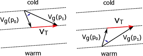
We can learn a lot from the thermal wind (seen in the figure above).

• Thermal wind blows with cold air to the left (on average) and with the warm air on the right in the Northern Hemisphere (remember “air is light on the right”), and with warm air on the left in the Southern Hemisphere.
• If the geostrophic wind vector rotates counterclockwise with height (called backing), then there is cold air advection. For the Northern Hemisphere, remember “CCC: counterclockwise cold.”
• If the geostrophic wind vector rotates clockwise with height (called veering), then there is warm air advection.
• In the Northern Hemisphere, because low thickness means lower layer temperature and higher thickness means higher layer temperature, the thermal wind blows parallel to the lines of constant thickness [10] with the low thickness on the left.
• This statement is an analogy to “The geostrophic wind blows parallel to the height contours on a pressure surface (pressure contours on a height surface) with the low height (pressure) to the left."

Summary

Understanding atmospheric dynamics is built upon three conservation laws: energy (the 1st Law of Thermodynamics), mass, and momentum. When we use conservation of momentum on the rotating Earth, we need to consider not only the real forces of gravity, pressure gradient force, and turbulent drag in the lower troposphere, but also apparent forces—centrifugal and Coriolis. With these terms, we can use conservation of momentum to write down the equations of motion in the Earth's reference frame and then show how they can be transformed into spherical coordinates or even pressure coordinates in the vertical and natural coordinates in the horizontal.

Using natural coordinates simplifies the equation of motion for geostrophic flow (the balance of Coriolis and pressure gradient forces), cyclostrophic flow (the balance of centrifugal and pressure gradient forces), inertial flow (the balance between centrifugal and Coriolis forces), and gradient flow (the balance among the pressure gradient force, Coriolis force, and horizontal centrifugal force). Upper air motion around high and low pressure causes upper-air convergence and divergence, which leads to high and low pressure at the surface.

Finally, the temperature decrease at each pressure level from tropics to the poles leads to a pressure gradient force that drives air toward the poles. The Coriolis force turns the air toward the east, creating westerlies observed in the midlatitudes of both hemispheres. This connection between the latitudinal temperature gradient and wind is expressed in the thermal wind equation. The thermal wind vector, which is the difference between the geostrophic winds at two different pressure levels, is parallel to isotherms, with cold air on the left in the Northern Hemisphere. If the geostrophic wind vector turns counterclockwise with height in the Northern Hemisphere, cold air advection is occurring in that layer of air. This relationship is a handy way to figure out if the advection is cold or warm.

Reminder - Complete all of the Lesson 10 tasks!

You have reached the end of Lesson 10! Double-check that you have completed all of the activities before you begin Lesson 11.