Lessons
This is the course outline.
Lesson 0: Introduction to Reactive Transport Modeling
Overview
This lesson introduces Reactive Transport Models (RTMs), primarily focusing on a brief history of RTM development, governing equations, and key concepts. It includes a lightboard video about the governing RT equations, a video that introduces the code that we will use in this class, CrunchFlow, and the reading materials here. The idea here is to give you an overview of RTM. Many concepts introduced here will be detailed in later lessons so it is OK if you do not fully grasp them in this lesson.
Please note that this is not a course that teaches how to numerically solve for reactive transport equations, which deserve a separate course by itself. Instead, this is a course that teaches fundamental reactive transport concepts and how to use an existing software CrunchFlow to solve and answer specific questions. So this is a model application course, not a numerical method course.
Learning Outcomes
By the end of this lesson, you should:
- Know the RTM development history and recognize the names of general available reactive transport codes;
- Understand what RTMs do in a broad sense and how they are different from other types of models ;
- Gather what you need to run CrunchFlow simulations;
- Run CrunchFlow simulations using the provided example input and database files.
There are example files and hw files in each lesson (almost). If you would like extra exercise files, click here [1].
Lesson Roadmap
| (Optional) Reading |
Note: these are your references. You can skip through quickly in this lesson to get some overview idea. You will use these again and again later. |
|---|---|
| To Do |
|
Questions?
If you have any questions, please post them to our Questions? discussion forum (not e-mail), located in Canvas. I will check that discussion forum daily to respond. While you are there, feel free to post your own responses if you, too, are able to help out a classmate.
0.1 History of reactive transport modeling
Reactive transport models have been applied to understand biogeochemical systems for more than three decades (Beaulieu et al., 2011; Brown and Rolston, 1980; Chapman, 1982; Chapman et al., 1982; Lichtner, 1985; Regnier et al., 2013; Steefel et al., 2005; Steefel and Lasaga, 1994). Multi-component RTMs originated in the 1980s based on the theoretical foundation of the continuum model (Lichtner, 1985; Lichtner, 1988). RTM development advanced substantially in the 1990s with the emergence of several extensively-used RTM codes, including Hydrogeochem (Yeh and Tripathi, 1991; Yeh and Tripathi, 1989), CrunchFlow (Steefel and Lasaga, 1994), Flotran (Lichtner et al., 1996), Geochemist’s Workbench (Bethke, 1996), Phreeqc (Parkhurst and Appelo, 1999), Min3p (Mayer et al., 2002), STOMP (White and Oostrom, 2000), TOUGHREACT (Xu et al., 2000), among others (Ortoleva et al., 1987, Bolton, 1996). Several early diagenetic models were developed at similar times, including STEADYSED (Van Cappellen and Wang, 1996), CANDI (Boudreau, 1996), and OMEXDIA (Soetaert et al., 1996). These codes can be easily found through google their names.
RTMs are distinct from geochemical models that primarily calculate geochemical equilibrium, speciation, and thermodynamic state of a system (Wolery et al., 1990). RTMs also differ from reaction path models (Helgeson, 1968; Helgeson et al., 1969) that represent closed or batch systems without diffusive or advective transport. The major advance of modern RTMs was to couple flow and transport within a full geochemical thermodynamic and kinetic framework (Steefel et al., 2015).
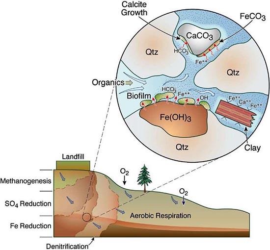
RTMs have been used across an extensive array of environments and applications (as reviewed in MacQuarrie and Mayer, 2005; Steefel et al., 2005). One primary focus has been in the low-temperature (ca < 100˚C) surface and near-surface environment where “rock meets life”, a region often referred to as the Critical Zone (CZ). Within the critical zone, water, atmosphere, rock, soil, and life interact creating the potential for complex chemical, physical, and biological interactions and responses to external forcing. As illustrated in Figure 0.1, RTMs can simulate a wide range of processes in this environment, including fluid flow (single or multiphase), solute transport (advective, dispersive, and diffusive transport), geochemical reactions (e.g., mineral dissolution and precipitation, ion exchange, surface complexation), and biogeochemical processes (e.g., microbe-mediated redox reactions, biomass growth and decay).
RTMs with these capabilities have been applied to understand chemical weathering and soil formation in response to various biological, climatic and physical drivers. RTMs have also been essential to address a wide range of questions at the nexus of energy and the environment, including, for example, environmental bioremediation (Bao et al., 2014), natural attenuation (Mayer et al., 2001), geological carbon sequestration (Apps et al., 2010; Brunet et al., 2013; Navarre-Sitchler et al., 2013), and nuclear waste disposal (Saunders and Toran, 1995; Soler and Mader, 2005). Model frameworks have advanced to incorporate heterogeneous characteristics of natural systems to begin to understand the role of spatial heterogeneities in controlling flow and the interaction between water and reacting components (Scheibe et al., 2006; Yabusaki et al., 2011; Liu et al., 2013). With the expansion of isotopes as tracers of mineral-fluid and biologically mediated reactions, recent advances include development of RTMs that allow an explicit treatment of isotopic partitioning due to both kinetic and equilibrium process.
The RTM approach has also been used to investigate subsurface processes at spatial scales ranging from single pores (Kang et al., 2006; Li et al., 2008; Molins et al., 2012) and single cells (Scheibe et al., 2009; Fang et al., 2011), to pore networks and columns (1 -10s centimeters) (Knutson et al., 2005; Li et al., 2006; Yoon et al., 2012; Druhan et al., 2014), and to field scales (1-10’s of meter) (Li et al., 2011), with a few studies at the watershed or catchment scale (100s of meters) (Atchley et al., 2014). Recent weathering studies have linked regional scale reactive transport models (WITCH) to global climate models to understand the role of climate change in controlling weathering (Godderis et al., 2006; Roelandt et al., 2010). Recent model development also includes full coupling between subsurface biogeochemical processes and surface hydrology, land-surface interactions, meteorological and climatic forcings (Bao et al., 2017; Li et al., 2017a). Such coupling has been argued to be important in understanding the complex interactions between processes of interests in different disciplines (Li et al., 2017b).
0.2 Reactive transport equations and key concepts
Most reaction transport codes solve equations of mass, momentum, and energy conservation (Steefel et al., 2005). For mass conservation, reactive transport models usually partition aqueous species into primary and secondary species (Lichtner, 1985). The primary species are the building blocks of chemical systems of interest, upon which concentrations of secondary species are written through laws of mass action for reactions at thermodynamic equilibrium. The partition between primary and secondary species allows the reduction of computational cost by only solving for mass conservation equations for primary species and then calculating secondary species through thermodynamics. Detailed discussion on primary and secondary species will be in lesson 1 on Aqueous Complexation.
Please watch the following video: Reactive Transport Reactions (7:25)
Click for a transcript of the Reactive Transport Reaction video
Reactive Transport Reactions
PRESENTER: What I'm going to do today is really to introduce the general idea of reactive transport equation and the overview of it. This equation that I put here is we call mass conservation equation for chemical species in aqueous phase, for one of the representative species. I don't expect you to know every term, or the details of every term in this equation. Because we will be talking more about each term later. But this is really to give you a general idea and overview before we start about everything.
And the importance of this is that we run these reactive transport codes. And there are a lot of built up architecture behind the code, in terms of what they solve. And it's always a good idea to know some of these, like what they solve, and what are the things behind these codes. So what I will do today is really talk through each of these terms and talk about the [? fake ?] meaning of each term, so that you get a general idea what are they really for.
So the first term we call the mass conservation term. It's called mass accumulation rate. And it should have the units of mol per length cubed, which is volume, of porous media per time, whatever time you pick. But all the terms have to be consistent, have the same length and time units. So this equation really says mass accumulation rate depends on several different processes, right?
So the first term is the rate itself. And the overall rate, the second term, what we call dispersive and diffusive transport. So you think about how a chemical species in water has a change over time, which is this. So some of these rates coming from, for example, the chemical species gold to get different concentrations in different locations. For example, you think about a dye put in a cup of water. And over time, they tend to have the same color everywhere. So this is one of the driving forces, in terms of what we call diffusive or dispersive transport. And they should have the same unit as the first term. Every term should have the same unit. So that's a second term.
And then, the third term is what we call the advective transport. And this is a process where, for example, you think about rivers, right? And the chemical species will flow together with the water. And so essentially, the water brings the chemical species to different places. So this advective transport, in this term, you have the hue, which is we call Darcy velocity. And then, the concentration actually I probably should explain here, the Ci will be the concentration of one chemical species of species i, a representative species, i. And the Ci everywhere is the same. So this is advective transport.
But also in a lot of systems, you have reactions, right? So the last term, four, is for the total reaction rates. And again overall, it has the same units as the first term. But essentially, this could it be a summation of several different-- let's call this equal to summation of i, which is for the chemical species, i. But this i could be involved in, let's say, ik, different numbers of reactions. So essentially, you will be adding all these reactions that this can chemical species, i, is participating in. And this ik would be a total number of reactions.
OK, so this is one representative equation. We write this equation form for the species, i. But I put the i from 1 to n here, meaning you can have any arbitrary number of what we call a primary species. So if you have, let's say, 10 different chemical species, then the primary species you have n equal to 10. And you will be writing 10 of these equations.
And these equations, essentially, if we solve these equations, you get the concentration or different chemical species as a function of time and space. So essentially, the outcome of this is the temporal and spatial distribution of chemical species. So essentially, you can tracing after each chemical species and look at how they change as a function of time and space and how, in different parts, they have different rates, and all that. Species i and i from 1 to n.
OK, so that's what you hope you guys will be exposed to in using this code. You will be solving this equations for particular, specific questions, problem applications. And then, you're usually given a set of initial conditions, like where is the concentration of different species at time 0 at different locations, and then over time, how these countries have different species evolve over time. And you will see you will learn a lot about these, using this code. And we'll be talking more about this in each of these terms, what are they, over time in different lessons that will follow.
The following is a representative mass conservation equation for a primary species I in the aqueous phase:
Here Ci is the total concentration of species i (mol/m3 pore volume), t is the time (s), n is the number of primary species, D is the combined dispersion–diffusion tensor (m2/s), u (m/s) is the Darcy flow velocity vector and can be decomposed into ux and uz in the directions parallel and transverse to the main flow direction. Nr is the total number of kinetic aqueous reactions that involve species i,
Equation (1) implies that the mass change rate of species i depends on physical and chemical processes: the diffusion/dispersion processes that are accounted for by the first term of the right hand side of the equation, the advection process that is taken into account by the second term of the right hand side, and reactions that are represented by the last term of the equation. The last term is the summation of multiple reaction rates, the form of which depend on the number and type of kinetic reactions that species i is involved in. The reaction terms include the rates of kinetically controlled reactions including microbe-mediated bioreduction reactions, mineral dissolution and precipitation reactions, and redox reactions. The reactions also include fast reactions that are considered at thermodynamics equilibrium, including aqueous complexation, ion exchange, and surface complexation. These fast reactions that are at equilibriums however do not show up in the above governing equation (1). Instead they exhibit themselves in the non-linear coupling of primary and secondary species through the expression of equilibrium constants (laws of mass action), as will be detailed later.
The dispersion-diffusion tensor D is defined as the sum of the mechanical dispersion coefficient and the effective diffusion coefficient in porous media D*(m2/s). At any particular location (grid block) with flow velocities in longitudinal (L) and transverse (T) directions, their corresponding diffusion / dispersion coefficients DL (m2/s) and DT (m2/s) are calculated as follows:
Here αL and αT are the longitudinal and transverse dispersivity (m). The dispersion coefficients vary spatially due to the non-uniform distribution of the permeability values.
As will be discussed in lesson 1, in a system with N total number of species and m fast reactions, the total number of primary species is n = N – m. With specific initial and boundary conditions, reactive transport codes solve a suite of n equation (1) with explicit coupling of the physical processes (diffusive/dispersive + advective transport) together with m algebraic equations defined by the laws of mass action of fast reactions. The output is the spatial and temporal distribution of all N species. This type of process-based modeling allows the integration of different processes as a whole while at the same time differentiation of individual process contribution in determining overall system behavior.
0.3 Course Structure
The focus of this course is on how to use an existing reactive transport code, not on how to numerically solve reactive transport equations, which deserves a separate course by itself. Readers who are interested in numerical methods of RTM are referred to book chapters and literature for details of discretization of the equations and numerical solution.
The rest of the course is structured as follows. Unit 1 includes lessons that teach principles and set up of geochemical reactions in well-mixed systems (zero-dimension in space, well-mixed systems). In this unit, the equations solved are ordinary differential equations (ODEs) with time as the independent variable however without space dimensions. Lesson 1 focuses on the concepts of primary and secondary species, reaction thermodynamics, and aqueous complexation reactions. Lesson 2 teaches mineral dissolution and precipitation reactions and Transition State Theory (TST) rate law. Lesson 3 is on surface complexation reactions. Lesson 4 teaches ion exchange reactions. Lesson 5 teaches microbe-mediated reactions.
Unit 2 teaches principles and set up of solute transport processes. This is where we introduce the space dimension. Here we solve Advection-Dispersion equation (ADE) without reactions in a one-dimensional system (lesson 6). Lesson 7 teaches principles and set up of heterogeneous, two dimensional domains.
Unit 3 combines biogeochemical reactions in Unit 1 and solute transport processes in Unit 2. Lesson 9 is an example of 1D transport with multiple mineral dissolution and precipitation reactions. If you run the simulation sufficiently long and allow the properties change over time, it becomes a chemical weathering simulation. Lesson 9' intends to have you combine solute transport with microbe-mediated reactions based on lessions 5 and 6. Lesson 10 introduces a 2D system with both physical and geochemical heterogeneities.
0.4 CrunchFlow
CrunchFlow was developed by Carl I. Steefel [2] in the 1990s (Steefel and Lasaga, 1994). It has been continuously evolving with new capabilities and features. Please refer to the CrunchFlow webpage for detailed introduction of code capabilities [3]. Among various existing reactive transport code, we choose to teach CrunchFlow owing to its features that allows each incorporation, computational efficiency with the use of fast solvers from the petsc (Portable, Extensible Toolkit for Scientific Computation) library, and its flexibility in simulating spatailly heterogeneous systems.
CrunchFlow executables: There are several different versions of CrunchFlow executables in Canvas. They are for different operation systems: windows – 32 bit, windows – 64 bit, and Mac. Please download the version that is compatible to the operating system on your PC. For windows executables, you need a dynamic library (.dll file) to run the exe, which is also in the corresponding Canvas folder. The Mac executables do not need a dynamic running library.
CrunchFlow Orientation:
- CrunchFlow - a reactive transport code
- For windows, you need to have these files run Crunchflow: executable file (.exe), a dll file (.dll), an input file (.in), a database file (.dbs)
- Input file: contains information the code need to set up the systems
- Database file: includes information related to reaction stoichiometry, reaction equilibrium constants, and reaction rate parameters
In input file:
- Comments should start with “!” and start from the beginning of the line, not middle of the line.
- Do not use Tab. Use space if you need to lay out things neatly.
- Output files from early runs will be overridden by later runs. Keep output files from different runs in different folders if you would like to have a record. Please use the folder name that self explains so that you know the content of different runs easily.
- Search CrunchFlow manual for the syntax of keywords.
- The exercises in the exercise folder are complementary to examples that we go through.
Please watch the video (32:46 minutes) Lesson 0 Crunch Flow Orientation that introduces CrunchFlow and its database and input file structure.
PRESENTER: Let's talk about the CrunchFlow. So this short video is supposed to be orientation for CrunchFlow. I introduced in the lesson, in the orientation lessons, that there are a lot of other reactive transport codes. Besides CrunchFlow, you have TOUGHREACT, PFLOTRAN, PHREEQC, [INAUDIBLE]. Different reactive transport has a bit of different flavors, but they all solve similar mass conservation equations for different species.
So the backbone of different reactions code are the same. But they have different solvers. They could have different computational speed because of use of different solvers. Also, using different solvers, it could have different convergence capabilities. So the way it's numerically solved, it could be very different. And that directly determines how fast things are going to run in your system.
I choose to teach CrunchFlow for several reasons among all of these other reactive transport codes. Mostly because I think it's very flexible in terms of setting up At the beginning, the learning curve might be a little bit-- you might think it's a bit sharp because of it's not a GUI interface. It's not graphic. And you might not be used to text file and opening objects exactly. But once you get used to it, this allows you a lot of flexibility to run things and put in things that are much faster than a lot of other reactive transport code does.
And also, it uses advanced solver like this [INAUDIBLE] package which has a lot of fast solvers. package was developed in a national lab. I believe it's Argonne, if I remember correctly. So it runs fast. And it tends to be robust. It usually doesn't get into non-convergence problem unless your system is ill conditioned or there's a bit of somewhere, there's a bug there.
But then it also is very flexible in terms of setting up heterogeneous systems. Like if you have different low permission, high permission, some mineral in somewhere that is more abundant than in other locations and less abundant, you can act expressly set it up in CrunchFlow, which I think it's the biggest advantage for CrunchFlow.
So in order to be able to run CrunchFlow, you need-- actually, so in this class, I put all the different executables on the course website. So there's also the manual files. There's a folder of CrunchFlow exercises which has a lot of different files there that [INAUDIBLE], when he taught CrunchFlow short courses before, he tended to use these exercise files.
So you can see these exercises in addition to what we teach here. And if at the end, we are running your project, you will be looking for things that you can use. And those exercises could be a very nice complementary in terms of adding additional examples and template input files for you to use.
So I think in these classes, when you try to learn CrunchFlow, you should use the menu frequently. You can search for the keywords and look at the explanation. You don't have to read everything at the beginning because I think that doesn't-- if you do that, the information doesn't register as much because you haven't gotten much of a handle on understanding the code yet. So I always advertise, learn it when you use it. I think that's where the information registers the best.
So what I have here is a folder that has four files-- so executable CrunchTope 64-bit for the Windows system I have. There's a DLL. There's the input file and DBS file. So these four files are the necessary files in order to run the CrunchFlow in a folder. You can not just set up exactly in the system to make it run default without copying to different folder. But for now, let's just keep it simple and keep it in this folder.
So we have this example, which we knew is a family of the CrunchFlow executable. It's called now CrunchTope because it actually incorporated isotope geochemistry. So the code should be able to run isotope information and everything.
This DLL file is a library file. How the code does is when it's solving the equations, it actually calls some dynamic library. So this library file is necessary in order for the code to finish. And then you have the input file and the database file.
So we are going to introduce these two files a bit just to introduce the structure of it. I'm not going to talk about it in detail, but just give you kind of a sense of what's going on. And then in the later lessons, most of the keywords will be introduced. And you learn by working on exercises and examples.
So the input file is mostly divided into keyword blocks. For example, here you have title block, which you can have a name and introduce what is this input file about it. It's good record keeping. Every keyword block, typically tried to differentiate keyword block name and keyword. So you use a capital to indicate the keyword block names. So it's easier to see. And keyword block should end with an END, like what we have here.
So typically, this is flow and transport in 1D system. So there's multiple keyword blocks here. There's RUNTIME, there's OUTPUT, DISCRETIZATION, and all that. Today, I probably will just introduce the RUNTIME mostly.
A lot of these keywords, it's related to a numerical solution process. Typically, I don't suggest changing early on because you might-- whatever default that you use it. One thing that's sometime useful is this specifies a solver, just name a solver. So those several different solvers if you look up in the menu. Several different solvers, you potentially can change one to the other if you have, for example, non-convergence problem at some point.
There's a pc, pclevel. They're all explained in CrunchFlow. So typically when I do it, I tend to kind of open the manual and I learn it. I tend to look at all that and try to learn what it means, why I'm using that, for example, pclevel, pc, pclevel. So the manual explains what it means. So you can dig into that and do things.
And one thing that is important to keep in mind is for you not to put in comments. For example, there's a line you want to explain what the number is from and what it means and what are units and everything. You can use a command line starting with this, exclamation mark.
You cannot do exclamation mark in the middle of line, for example, like doing this this. The code is not going to recognize. So you always need to start a new line with starting with the exclamation mark to do comments. So the code will be actually read as a text not as a keyword.
One thing it's important to keep in mind is your name of database file need to the exact same as the name of a database file in the same folder. For example, here we have datacom.dps. You should put that there. If you put another name there and then you don't have that database in this folder, then it's not going to run. Or if you have multiple databases in the same folder, you need to specify which one you are going to use.
These are the different ways of solving. So screen output is the number of steps that you skip before the screen actually has an output. If it's one, it's putting up every timestamp. If it's 10, it's putting up every 10 timestamps.
And then there's OUTPUT keyword block. You can putting time unit like minutes, seconds, hours, et cetera. So this is the time. You can put several times you want to see the snapshot of the system. And the last one is how long the system is going to run to. So in this system, it's going to run to 250 minutes.
Time series is where you want to have, for example, in a particular grid block, you want to have a times series from time beginning to end of simulation. You want to see how the concentration, for example, evolve over time. So that's the name of the output file that is going to have that information. And this specifies which grid block you want to have that time series. You can do multiple times series with different names and different grid blocks.
And this time set interval determines how fast-- how many-- like every once or every time step the code is going to write on the breakthrough curve. If you want that output for every 10-- every 10 times timestamps, that's fine too. Then it makes the breakthrough file a bit smaller because you have less output. Anyway, so this is output.
I'm not going to introduce everything else in the system because we will be introduced in detail all the keyword blocks in one of the lessons on 1D physical process, with diffusion dispersion process. So I'm going to leave these to there for the introduction of these blocks.
So all we teach of this is more or less get familiar with the keywords for each different process. What do you need to do in order to setting up this meaning for it and making sense.
Now before we close, let's talk about the database. So this datacom. This is a long file. And it's borrowed from EQ3 database, essentially. It started with a line called temperature points. So these are different. There are eight different temperature points.
If you want to understand what are the details, for example, there are eight different temperature points. These are for different degree Celsius. So there's log K when we talk about it. This is a reaction, different reactions at eight different K values corresponding to the eight different temperatures, which is already done in the EQ3/6.
So if you are specifying temperature is 150, the code is going to read the log K value for the different reactions from the fifth number, not from the default 25 degree Celsius. That's what it's for. So that's the temperature point.
These are the Debye-Huckel coefficients. Because the code uses the Debye-Huckel equation to calculate activity coefficients. And then starting after the Debye-Huckel block, you have from starting from water should be end of primary. So the answer from up until here, it's a list of primary species.
And each primary species has three parameters there. The first one is the Debye-Huckel parameters that you can use for that species. This is charge. And this is molecular weight for all the different primary species. So you can actually add in your own primary species if you use artificial makeup and elements or something. So sometimes, you need to manipulate code to do something that you want. There should be a presence in the primary species because the primary species is essentially the building block of the system.
So after primary species, you would have, starting from the line-- following the end of primary, you will start to have the secondary species. So all these secondary species are written, for example, like this. Let's look at HS.
So for the relevant primary species for the sulfide species is a sulfate. It didn't exist in this database. You actually can put in another sulfide if you want. But here, the primary species here is sulfate. So there's no sulfides there. You can do the sulfide species when you give it another name. So you can specify the sulfide species as written in terms of redox reaction with oxygen. So a sulfide becomes reduced to become sulfide. Or it's just plus O2 gas to become sulfate being oxidized.
Let's look at another maybe bicarbonate or something. For carbonates, look at carbonate. For carbon species, what you specify in the system is-- here, this CO2. There should be a CO2. Let's see. Let's search for. Oh, yeah. There's a bicarbonate there. So the bicarbonate is a primary species.
And then everything else, for example, CO2 aq or bicarbonate should be written as bicarbonate. So here when it's-- so let's look at this line specifically. This is essentially writing CO3 bicarbonate species. It involved two different species. One is hydrogen ion. The other is bicarbonate.
So if you write it, it'd be CO3 minus minus plus. When it's minus meaning it's in left hand side of equation. Plus equals two bicarbonate. So the primary species need to be in the right hand side.
And what are these? So these should be the equilibrium constants. These are not the right equivalent constant. It's the equivalent constant for following the way the reaction is written. So it's saying, bicarbonate species can be-- if you write it that way, it will be 9.6 log K.
This is the log K value. So this is not 10.03, which means it's at a different temperature. And it's using the same value. So it's not corresponding to the temperature.
So if you want to look at a temperature effect, every reaction, later on when you're writing, you will need to specify. If you are actually running high temperature, you want to look up this number to make sure this number in database is correct, just to confirm because sometimes these databases are changed by people. So you want to make sure the numbers are right. Because these are very important numbers.
If we look at CO2 aq, it's essentially saying CO2 aq plus water equals H plus and bicarbonate. So there's three species involved. And for this reaction, you have the log K equal at zero is minus 6.58. And at high temperature, it keeps on decreasing. So this set of numbers is making sense.
But you still want to check. Every number you use and you end up using in the modeling process, you want to check these numbers. So 3.0 is, again, is the Debye-Huckel. So these three numbers is essentially like the same three numbers as used in the primary species. It was Debye-Huckel parameters, charge, and molecular weight. So that's the list of secondary primary.
And I do Control-F, I will see end of secondary. So it will say end of secondary. This is towards the end of the secondary species list. Everything in secondary species is written in terms of primary species. And then you see a block of everything with a g. Process g means a gas phase. So all the gas phases are listed here. And then there should be an end of gases. These are end of gases.
And then after that, after gases, you would have all these mineral phases. So you can see the different reactions, different-- let's search for calcite. Calcite, so again, for the calcite, you have molecular weight. The reaction written in terms of two species. This is a stoichiometric coefficient, one calcium and one carbonate.
And again, you have these are the log K. Again here, the value is not necessarily right because you have all the same. But I believe this number should be the log K equals at 25 degrees Celsius.
For the mineral phase, you only have molecular weight. You don't have Debye-Huckel and charge because these are not in the water for aqueous phase. So then this should be-- so each mineral is written this way. So if you go to end minerals, it's the end of mineral phase.
And then it will begin the surface complexation session. It will specify the way surface complexation is written as well as, again, this is a reaction. And then this log K value in different conditions. Every time you see all the 500.000, these are numbers that are kind of dummy numbers that you put in because you don't know what number to use.
So this number means if you are looking, for example, at this here, we know that 25 degree Celsius log K for this reaction is 8.82. But for all other temperatures, we don't know. So if you need to use at these other temperatures, you need to look it up in the literature. And then this ending end of surface complexation.
Now the other thing I want to point out is there's also surface complexation at end. So there's the beginnings of the complexation parameters that give you the charges of the different surface species. So these are actually the surface charges of the surface reactions directly related to surface complexation. So this is surface complexation.
Then you have aqueous kinetic block and then mineral kinetic block. Again, I always suggest that you will be looking up literature for real numbers. For example, let's say here you are specifying, let's look at calcite again as an example.
So for example for calcite here, it's specified several different brick blocks for different [INAUDIBLE]. So every one has a label. In this block, the label default and you are actually looking at this reaction and with dependence on H plus. Here, it didn't specify dependence, so it should be-- it says no dependents here.
Like here, it will be dependence active to H plus raised to 1.0. And this would read, constant activation energy, the type of [INAUDIBLE] used, and all that. And for the other one, for this one, you're saying is dependent on CO2 aq to the 1.0 for the calcite dissolution reaction. So some figure them somewhere else, you also write pyrite oxidation reaction and you have all these.
So you can also in the input file put the rate constant like this. So if you're putting input files your rate constant, then it's going to ignore what you have in the database and use the one in the input file. Anyway, so that's for the mineral kinetics.
And if the mineral that you are interested in is not already there, you can add another block specifying all these numbers. And as long as you specify, for example, the mineral is part of the mineral list, if you have a new mineral that is not in the list, you can add that in in the mineral list which specifies a reaction's log K values for that mineral. And then you add another mineral block for the kinetics here. So that's for the mineral kinetics.
And then you would have the exchange block, you can specify a multiple site ion exchange or a single site ion exchange. These are specified, essentially. Again, the reactions for the half life ion exchange reaction the exchange coefficient.
So after this, at the end, you have this. After this, so later part, you have some numbers These tend to be [INAUDIBLE]. You want to move around a little bit, you can just temporary start there. So you can more or less ignore this line if you want. I could just remove all that.
So let's do just a run. So what you do is when you try to run control, you click on the executable file. And then you will be putting the name. It will ask for the name of the input file transport. 1D.ing. You always have your input file in .ing so that the code recognizes it's the input file.
Now, after this you see a lot of more files. Because with all these, you should look at extension. All these output file are the output. So because I specify in the special profile one time, it will be output at Z1 time for all the different velocity, for the total concentration which we'll be talking that later, total concentration speciation, pressure, gas, concentration. And there's also an isotope file, and also a breakthrough curve because I want this time series. So you will see a lot of these output files.
If you change your input file at this point to a, let's say it's such and such a number, and rerun again here, the new output file will replace the old output file. So if you want to keep a record of both, you need to have another folder to run the simulation in order to make it be able to kind of compatible to still have the record of each. Otherwise, it's going to be overwritten.
Let's look at transport 1D out. It's essentially kind of echoes what has been [INAUDIBLE]. It's essentially going through the file to see the input file and kind of keep a record of what has been [INAUDIBLE]. And then at end, it says, OK, I'm going to stop starting, initialization completed, starting timestamping.
So sometime if the code has stopped running in the middle or something, you can look at this file to see if everything has been written in correctly. If not, that means there's something wrong in your input file. Another thing to keep in mind is in your input file, you're not supposed to the use tab. You have to space if you want to have things lay out nicely and everything. Don't use tab. The code doesn't recognize tab.
Let's look at the breakthrough. So here what we specify is the species bromide. So this is essentially for the [INAUDIBLE] cell, which is at outlet. You have time. You have bromide concentration. So early on, they'd run very-- because I put one [INAUDIBLE] for time interval. So it run every timestamping. So early on, it's like starting from 10 to minus 10 minutes. It's essentially initial condition. You don't have any bromide. And then in the input file, in that you inject input files, as the bromide [INAUDIBLE]. So you start to have higher and higher concentration at some point later.
So the inner concentration is this. So at somewhere, for example, around maybe 100 minutes or something, you start to have something come out. And then eventually this concentration stabilized to the end. So this is a system of just transport.
And these should be the log concentration. This is the concentration of bromide and log concentration. So this runs. And if you need to end this concentration, total concentration, for this non-reactive species, it's not really important.
So I'm going to stop here. And hopefully you have a bit of a sense of what's going on. Several things that you should remember is you always need the executable file, database, input file, and the library file to run the simulation. And the CrunchFlow manual will be your good friend in this class, besides the reading materials that you will learn about the general principles.
I'm going to stop here. So from Lesson One, we'll introduce four individual processes, what are the important keywords and parameters, and we'll go through exercises, and then run some simulations, do homework to kind of re-emphasize what you have learned in class. All right. That's what do we have for--
References
Apps, J. A., L. Zheng, Y. Zhang, T. Xu and J. T. Birkholzer (2010). "Evaluation of Potential Changes in Groundwater Quality in Response to CO2 Leakage from Deep Geologic Storage." Transport in Porous Media 82(1): 215-246.
Atchley, A. L., A. K. Navarre-Sitchler and R. M. Maxwell (2014). "The effects of physical and geochemical heterogeneities on hydro-geochemical transport and effective reaction rates." Journal of Contaminant Hydrology 165(0): 53-64.
Bao, C., H. Wu, L. Li, D. Newcomer, P. E. Long and K. H. Williams (2014). "Uranium Bioreduction Rates across Scales: Biogeochemical Hot Moments and Hot Spots during a Biostimulation Experiment at Rifle, Colorado." Environmental Science & Technology 48(17): 10116-10127.
Bao, C., Li, L., Shi, Y. and Duffy, C. (2017) Understanding watershed hydrogeochemistry: 1. Development of RT-Flux-PIHM. Water Resources Research 53, 2328-2345.
Beaulieu, E., Y. Goddéris, D. Labat, C. Roelandt, D. Calmels and J. Gaillardet (2011). "Modeling of water-rock interaction in the Mackenzie basin: Competition between sulfuric and carbonic acids." Chemical Geology 289(1–2): 114-123.
Bethke, C. (1996). Geochemical reaction modeling : concepts and applications. New York, Oxford University Press.
Bolton, E. W., A. C. Lasaga and D. M. Rye (1996). "A model for the kinetic control of quartz dissolution and precipitation in porous media flow with spatially variable permeability: Formulation and examples of thermal convection." Journal of Geophysical Research: Solid Earth 101(B10): 22157-22187.
Boudreau, B. P. (1996). "A method-of-lines code for carbon and nutrient diagenesis in aquatic sediments." Computers & Geosciences 22(5): 479-496.
Brown, B. and D. Rolston (1980). "Transport and transformation of methyl bromide in soils." Soil science 130(2): 68-75.
Brunet, J. L., L. Li, Z. T. Karpyn, B. Kutchko, B. Strazisar and G. Bromhal (2013). "Dynamic evolution of compositional and transport properties under conditions relevant to geological carbon sequestration." Energy & Fuels.
Chapman, B. M. (1982). "Numerical simulation of the transport and speciation of nonconservative chemical reactants in rivers." Water Resources Research 18(1): 155-167.
Chapman, B. M., R. O. James, R. F. Jung and H. G. Washington (1982). "Modelling the transport of reacting chemical contaminants in natural streams." Marine and Freshwater Research 33(4): 617-628.
Druhan, J. L., C. I. Steefel, M. E. Conrad and D. J. DePaolo (2014). "A large column analog experiment of stable isotope variations during reactive transport: I. A comprehensive model of sulfur cycling and delta S-34 fractionation." Geochimica Et Cosmochimica Acta 124: 366-393.
Fang, Y., T. D. Scheibe, R. Mahadevan, S. Garg, P. E. Long and D. R. Lovley (2011). "Direct coupling of a genome-scale microbial in silico model and a groundwater reactive transport model." Journal of Contaminant Hydrology 122(1-4): 96-103.
Godderis, Y., L. M. Francois, A. Probst, J. Schott, D. Moncoulon, D. Labat and D. Viville (2006). "Modelling weathering processes at the catchment scale: The WITCH numerical model." Geochimica et Cosmochimica Acta 70: 1128-1147.
Helgeson, R. C. (1968). "Evaluation of irreversible reactions in geochemical processes involving minerals and aqueous solutions: I. Thermodynamic relations." Geochim. Cosmochim. Acta 32: 853–877.
Helgeson, R. C., R.M. Garrels and F. T. MacKenzie (1969). "Evaluation of irreversible reactions in geochemical processes involving minerals and aqueous solutions: II. Applications,." Geochim. Cosmochim. Acta 33: 455– 482.
Kang, Q. J., P. C. Lichtner and D. X. Zhang (2006). "Lattice Boltzmann pore-scale model for multicomponent reactive transport in porous media." Journal of Geophysical Research-Solid Earth 111.
Knutson, C. E., C. J. Werth and A. J. Valocchi (2005). "Pore-scale simulation of biomass growth along the transverse mixing zone of a model two-dimensional porous medium." Water Resources Research 41(7).
Li, L., N. Gawande, M. B. Kowalsky, C. I. Steefel and S. S. Hubbard (2011). "Physicochemical heterogeneity controls on uranium bioreduction rates at the field scale." Environmental Science and Technology 45(23): 9959-9966.
Li, L., C. A. Peters and M. A. Celia (2006). "Upscaling geochemical reaction rates using pore-scale network modeling." Advances in Water Resources 29(9): 1351-1370.
Li, L., C. I. Steefel and L. Yang (2008). "Scale dependence of mineral dissolution rates within single pores and fractures." Geochimica Et Cosmochimica Acta 72(2): 360-377.
Li, L., Bao, C., Sullivan, P.L., Brantley, S., Shi, Y. and Duffy, C. (2017a) Understanding watershed hydrogeochemistry: 2. Synchronized hydrological and geochemical processes drive stream chemostatic behavior. Water Resources Research 53, 2346-2367.
Li, L., Maher, K., Navarre-Sitchler, A., Druhan, J., Meile, C., Lawrence, C., Moore, J., Perdrial, J., Sullivan, P., Thompson, A., Jin, L., Bolton, E.W., Brantley, S.L., Dietrich, W.E., Mayer, K.U., Steefel, C.I., Valocchi, A., Zachara, J., Kocar, B., McIntosh, J., Tutolo, B.M., Kumar, M., Sonnenthal, E., Bao, C. and Beisman, J. (2017b) Expanding the role of reactive transport models in critical zone processes. Earth-Sci. Rev. 165, 280-301.
Lichtner, P. C. (1985). "Continuum Model for Simultaneous Chemical-Reactions and Mass- Transport in Hydrothermal Systems." Geochimica et Cosmochimica Acta 49(3): 779-800.
Lichtner, P. C. (1988). "The Quasi-Stationary State Approximation to Coupled Mass- Transport and Fluid-Rock Interaction in a Porous-Medium." Geochim. Cosmochim. Acta. 52(1): 143-165.
Lichtner, P. C., C. I. Steefel and E. H. Oelkers, Eds. (1996). Reactive transport in porous media. Reviews in Mineralogy, MIneralogical society of America.
Liu, C., J. Shang, H. Shan and J. M. Zachara (2013). "Effect of Subgrid Heterogeneity on Scaling Geochemical and Biogeochemical Reactions: A Case of U(VI) Desorption." Environmental Science & Technology 48(3): 1745-1752.
MacQuarrie, K. T. B. and K. U. Mayer (2005). "Reactive transport modeling in fractured rock: A state-of-the-science review." Earth-Science Reviews 72(3-4): 189-227.
Mayer, K. U., S. G. Benner, E. O. Frind, S. F. Thornton and D. N. Lerner (2001). "Reactive transport modeling of processes controlling the distribution and natural attenuation of phenolic compounds in a deep sandstone aquifer." Journal of Contaminant Hydrology 53(3-4): 341-368.
Mayer, K. U., E. O. Frind and D. W. Blowes (2002). "Multicomponent reactive transport modeling in variably saturated porous media using a generalized formulation for kinetically controlled reactions." Water Resources Research 38(9).
Molins, S., D. Trebotich, C. I. Steefel and C. Shen (2012). "An investigation of the effect of pore scale flow on average geochemical reaction rates using direct numerical simulation." Water Resources Research 48.
Navarre-Sitchler, A. K., R. M. Maxwell, E. R. Siirila, G. E. Hammond and P. C. Lichtner (2013). "Elucidating geochemical response of shallow heterogeneous aquifers to CO2 leakage using high-performance computing: Implications for monitoring of CO2 sequestration." Advances in Water Resources 53(0): 45-55.
Ortoleva, P., E. Merino, C. Moore and J. Chadam (1987). "Geochemical self-organization, I. Feedbacks, quantitative modeling." Am J Sci 287: 979–1007.
Parkhurst, D. L. and C. A. J. Appelo (1999). User’s guide to PHREEQC (Version 2)—A computer program for speciation, batch reaction, 1 dimensional transport, and inverse geochemical calculation: 310.
Regnier, P., S. Arndt, N. Goossens, C. Volta, G. G. Laruelle, R. Lauerwald and J. Hartmann (2013). "Modelling Estuarine Biogeochemical Dynamics: From the Local to the Global Scale." Aquatic geochemistry 19(5-6): 591-626.
Roelandt, C., Y. Goddéris, M. P. Bonnet and F. Sondag (2010). "Coupled modeling of biospheric and chemical weathering processes at the continental scale." Global Biogeochemical Cycles 24(2): GB2004.
Saunders, J. A. and L. E. Toran (1995). "Modeling of radionuclide and heavy metal sorption around low- and high-{pH} waste disposal sites at {Oak Ridge, Tennessee}." Appl. Geochem. 10(6): 673-684.
Scheibe, T. D., Y. Fang, C. J. Murray, E. E. Roden, J. Chen, Y.-J. Chien, S. C. Brooks and S. S. Hubbard (2006). "Transport and biogeochemical reaction of metals in a physically and chemically heterogeneous aquifer." Geosphere 2(4): doi: 10.1130/GES00029.00021.
Scheibe, T. D., R. Mahadevan, Y. Fang, S. Garg, P. E. Long and D. R. Lovley (2009). "Coupling a genome-scale metabolic model with a reactive transport model to describe in situ uranium bioremediation." Microbial Biotechnology 2(2): 274-286.
Soetaert, K., P. M. J. Herman and J. J. Middelburg (1996). "A model of early diagenetic processes from the shelf to abyssal depths." Geochimica et Cosmochimica Acta 60(6): 1019-1040.
Soler, J. M. and U. K. Mader (2005). "Interaction between hyperalkaline fluids and rocks hosting repositories for radioactive waste: Reactive transport simulations." Nuclear Science and Engineering 151(1): 128-133.
Steefel, C. I., C. A. J. Appelo, B. Arora, D. Jacques, T. Kalbacher, O. Kolditz, V. Lagneau, P. C. Lichtner, K. U. Mayer, J. C. L. Meeussen, S. Molins, D. Moulton, H. Shao, J. Šimůnek, N. Spycher, S. B. Yabusaki and G. T. Yeh (2015). "Reactive transport codes for subsurface environmental simulation." Computational Geosciences 19(3): 445-478.
Steefel, C. I., D. J. DePaolo and P. C. Lichtner (2005). "Reactive transport modeling: An essential tool and a new research approach for the Earth Sciences." Earth and Planetary Science Letters 240: 539-558.
Steefel, C. I. and A. C. Lasaga (1994). "A coupled model for transport of multiple chemical species and kinetic precipitation/dissolution reactions with application to reactive flow in single phase hydrothermal systems." Am. J. Sci. 294: 529-592.
Steefel, C. I. and A. C. Lasaga (1994). "A coupled model for transport of multiple chemical species and kinetic precipitation/dissolution reactions with application to reactive flow in single phase hydrothermal systems." American Journal of Science 294(5): 529-592.
Van Cappellen, P. and Y. F. Wang (1996). "Cycling of iron and manganese in surface sediments: a general theory for the coupled transport and reaction of carbon, oxygen, nitrogen, sulfur, iron, and manganese." Am J Sci 296: 197-243.
White, M. D. and M. Oostrom (2000). STOMP: Subsurface Transport Over Multiple Phases (Version 2.0): Theory Guide. Richland, WA.
Wolery, T. J., K. J. Jackson, W. L. Bourcier, C. J. Bruton, B. E. Viani, K. G. Knauss and J. M. Delany (1990). "CURRENT STATUS OF THE EQ3/6 SOFTWARE PACKAGE FOR GEOCHEMICAL MODELING." Acs Symposium Series 416: 104-116.
Xu, T. F., S. P. White, K. Pruess and G. H. Brimhall (2000). "Modeling of pyrite oxidation in saturated and unsaturated subsurface flow systems." Transport Porous Med 39(1): 25-56.
Yabusaki, S. B., Y. Fang, K. H. Williams, C. J. Murray, A. L. Ward, R. D. Dayvault, S. R. Waichler, D. R. Newcomer, F. A. Spane and P. E. Long (2011). "Variably saturated flow and multicomponent biogeochemical reactive transport modeling of a uranium bioremediation field experiment." Journal of Contaminant Hydrology 126(3-4): 271-290.
Yeh, G.-T. and V. S. Tripathi (1991). "A Model for Simulating Transport of Reactive Multispecies Components: Model Development and Demonstration." Water Resources Research 27(12): 3075-3094.
Yeh, G. T. and V. S. Tripathi (1989). "A critical evaluation of recent developments in hydrogeochemical transport models of reactive multichemical components." Water Resources Research 25(1): 93-108.
Yoon, H., A. J. Valocchi, C. J. Werth and T. Dewers (2012). "Pore-scale simulation of mixing-induced calcium carbonate precipitation and dissolution in a microfluidic pore network." Water Resources Research 48.
Summary and Final Tasks
Summary
In this orientation we have an overview of the history of RTM development and the applications of RTMs in the past decades. We also discussed general reactive transport equations and the physical meaning of different terms. At the end we introduce CrunchFlow, the code we will learn to use in this class.
Reminder - Complete all of the Lesson 0 tasks!
You have reached the end of Lesson 0! Double-check the to-do list on the Lesson 0 Overview page [15] to make sure you have completed all of the activities listed there. Please download CrunchFlow compatible with your PC, and run the example files following the instructions in the video. Please report any problems if it does not work so we can help you set up.
Lesson 1: Aqueous Complexation
Chemical species form complexes in the water phase through aqueous complexation reactions. These reactions occur fast and are controlled by reaction thermodynamics. This lesson introduces reaction thermodynamics, equilibrium constants, and how to set up simulations for aqueous speciation / metal complexation reactions in CrunchFlow. We will discuss thermodynamics principles, followed by the concepts of primary and secondary species. A few examples will be illustrated about how to choose primary and secondary species, and setup simulations for aqueous complexation in CrunchFlow.
Learning Outcomes
By the end of this lesson, you should be able to:
- Understand reaction thermodynamics principles
- Understand why and how to group different aqueous species into primary and secondary species
- Set up simulations for aqueous speciation and complexation reactions in CrunchFlow.
Lesson Roadmap
|
To Read (Optional) |
|
|
|---|---|---|
|
To Do |
|
|
Questions?
If you have any questions, please post them to our Questions? discussion forum (not e-mail), located in Canvas. The TA and I will check that discussion forum daily to respond. While you are there, feel free to post your own responses if you, too, are able to help out a classmate.
1.0 Aqueous complexation reactions
Example 1.1: A closed carbonate system. Imagine we have a closed bottle with clean water except with a head space filled with $\text{C}\text{O}_2$ gas. The system therefore only has carbonate species in the water phase, the pertinent reactions are as follows:
$$\mathrm{H}_2\mathrm{CO}_3^0\Leftrightarrow\mathrm{H}^++\mathrm{HCO}_3^-\quad K_{a1}=\frac{a_{H^+}a_{HCO_3^-}}{a_{H_2CO_3^0}}=10^{-6.35}$$
$$\mathrm{HCO}_3^-\Leftrightarrow H^++\mathrm{CO}_3^{2-}\quad K_{a2}=\frac{a_{H^+}a_{CO_3^{2-}}}{a_{\mathrm{_{ }HCO}_3^-}}=10^{-10.33}$$
$$\mathrm{H}_{2} \mathrm{O} \Leftrightarrow \mathrm{H}^{+}+\mathrm{OH}^{-} \quad K_{w}=a_{H^{+}} a_{O H^{-}}=10^{-14.00}$$
These are the speciation reactions between carbonate species and water species such as $\text{H}^+$ and $\text{OH}^-$. All these reactions are aqueous speciation reactions and occur fast. All Ks are equilibrium constants at standard temperature and pressure conditions. Note that here we are not imposing the condition for charge balance. Reactions in Example 1.1 are examples of aqueous complexation reactions. These reactions occur ubiquitously in water systems and have significant impacts on water chemistry. For example, ligands, dissolved organic carbon (DOC), and other anions can form complexes with cations, including metals, to prevent cations from precipitation, therefore increasing the mobility of cations in water systems. The carbonate complexation and dissociation reactions with $\text{H}^+$ in example 1.1 works as a buffering mechanism to prevent the pH of water from changing rapidly.
1.1 Reaction thermodynamics
Reaction equilibrium constants $K_{eq}$. Here we briefly cover fundamental concepts in reaction thermodynamics. For a more comprehensive coverage, readers are referred to books listed in reading materials [e.g., (Langmuir et al., 1997)]. A chemical reaction transforms one set of chemical species to another. Here is an example,
The reactants A and B combine to form the products C and D. The symbols $\alpha,\beta,\chi,\text{ and }\delta$ are the stoichiometric coefficients that quantify the relative quantity of different chemical species during the reaction in mole basis. That is, $\alpha$ mole of A and $\beta$ mole of B transform into $\chi$ mole of C and $\delta$ mole of D. The Symbol “$\text { É }$” indicates that the reaction is reversible and can occur in both forward and backward directions. According to reaction thermodynamics, the change in the Gibbs free energy $\Delta G_{R}$ during the reaction can be expressed as:
Here, $\Delta G_{R}^{0}$ is the change in reaction free energy under the standard condition (293.15 K and $10^5$Pa); R is the ideal gas constant (1.987 cal/(mol·K)); T is the absolute temperature (K); and $a_{A}, a_{B}, a_{C},a_{D}$ are the activities of the species A, B, C and D, respectively. The derivation of this equation goes to the heart of reaction thermodynamics theory. In any particular aqueous solution, we define ion activity product (IAP) for the reaction (1) as follows:
The reaction reaches equilibrium when the forward and backward reactions occur at the same rate, the point at which the change in the reaction Gibbs free energy $\Delta G_{R}$ reaches zero. At reaction equilibrium, the IAP equals to the equilibrium constant $K_{eq}$:
where $a_{A}, a_{B}, a_{C}, a_{D}$ are the activities of the species A, B, C and D at equilibrium, respectively. In general, larger $K_{eq}$ means larger reaction tendency to the right direction in the equation as written in (1). The $K_{eq}$ is a constant for a particular reaction at any specific temperature and pressure conditions. Although they look very similar, IAP is the ion activity product under any point along the reaction progress, while $K_{eq}$ is the IAP only at one particular point during the reaction, i.e., at equilibrium. We use the saturation index (SI) to compare IAP and $K_{eq}$:
When SI =0, the reaction is at equilibrium; when SI < 0, the reaction proceeds to the right (forward); when SI > 0, the reaction proceeds to the left (backward).
Dependence of $K_{eq}$ on temperature and pressure. Values of $K_{eq}$ are a function of temperature and pressure. According to reaction thermodynamics, the $K_{eq}$ dependence on temperature follows the Van’t Hoff equation under constant pressure:
Here, $\Delta V_{r}^{o}$ is the molar volume change of the reactions under the standard condition (cm3/mol). Typically, the effect of pressure is important when the reaction involves gas (e.g. $\mathrm{CO}_{2(g)}$) and when there is a significant difference in the molar volume of reactants and products.
If the $\Delta V_{r}^{o}$is a constant and does not depend on pressure, the integrated form the above equation is:
Where $K_{eq,1}$ and $K_{eq,2}$ are the equilibrium constants at P1 and P2, respectively. Typically, P1 is at atmospheric condition at 1 bar.
The standard thermodynamic properties (e.g. $H_{r}^{o}$ and $V_{r}^{o}$) of most compounds can be found or calculated from CRC handbooks (e.g., Handbook of Chemistry and Physics (Haynes, 2012), and the NIST Chemistry WebBook [16]. Readers are also referred to the standard geochemical database Eq3/6 for values of equilibrium constants (Wolery et al., 1990).
Biogeochemical reaction systems typically include both slow reactions with kinetic rate laws and fast reactions that are governed by reaction thermodynamics. Kinetic reactions include, for example, mineral dissolution and precipitation and redox reactions. Thermodynamically-controlled reactions are those with rates so fast that the kinetics does not matter for the problem of interest. In geochemical systems, these include, for example, aqueous complexation reactions that reach equilibrium at the time scales of milli-seconds to seconds. For these reactions, the activities of reaction species are algebraically related through their equilibrium constants, or laws of mass action, as shown in equation (4). As such, their concentrations are not independent of each other and should not be numerically solved independently. This necessitates the classification of aqueous species into primary and secondary species. The primary species are essentially the building blocks of chemical systems, whereas the concentrations of secondary species depend on those of primary species through the laws of mass action. As such, with the definition of primary and secondary species, a reactive transport code only needs to numerically solve the number of equations for the species that are independent of each other, which is essentially the number of primary species. The number of primary species is equivalent to the number of components in a system. The concentrations of secondary species can be calculated based on the concentrations of primary species using laws of mass action.
1.2 Primary and secondary species
Here we will go through a few examples on how we choose primary and secondary species using the tableau method. Details are referred to in chapter 2, Morel and Hering, 1993.
How do we categorize the primary and secondary species of the system? Here we go through several steps for the choice of primary and secondary species.
- What are the species?
List of species (5): H+, OH-, H2CO30, HCO3-, CO32-, (H2O is typically included implicitly).
- How many algebraic relationships do we have that define the dependence between activities of different species?
We have 3 fast aqueous reactions, which means that we have 3 laws of mass action, as shown in three expressions defining the equilibrium constant for each reaction.
- How many primary species do we have and what are they?
Here we have 5 species in total and 3 dependencies (equations). So we should have 5-3 = 2 primary species. The primary species should be defined so that all other secondary species can be written in terms of primary species.
- Can we choose H+ and OH- as primary species? No, because we cannot write the carbonate species as combinations of H+ and OH-,
- Can we choose H+ and CO32-? Yes. See the following table. The species in the top row are primary species. The first left column includes all species.
Species H+ CO32- (H2O) H+ 1< 0 0 OH- -1 0 1 H2CO30 2 1 >0 HCO3- 1 1 0 CO32- 0 1 0
We can write all species in terms of H+ and CO32-:
$$\begin{array}{l}
\mathrm{H}^{+}=\mathrm{H}^{+} \\
\mathrm{CO}_{3}^{2-}=\mathrm{CO}_{3}^{2-} \\
\mathrm{OH}^{-}=\left(\mathrm{H}_{2} \mathrm{O}\right)-\mathrm{H}^{+} \\
\mathrm{H}_{2} \mathrm{CO}_{3}=2 \mathrm{H}^{+}+\mathrm{CO}_{3}^{2-} \\
\mathrm{HCO}_{3}^{-}=\mathrm{H}^{+}+\mathrm{CO}_{3}^{2-}
\end{array}$$
Here ${OH}^{-}$, $\mathrm{H}_{2} \mathrm{CO}_{3}{}^{0}$, and ${HCO}_{3}^{-}$ are secondary species.
- Is the choice of primary species unique? No. As long as the secondary species can be written as combinations of primary species, the list is legitimate. For example, we can also use OH- and $\mathrm{HCO}_{3}$ as primary species in this example.
| Species | OH- | HCO3- | (H2O) |
|---|---|---|---|
| H+ | -1 | 0 | 1 |
| OH- | 1 | 0 | 0 |
| H2CO3 | -1 | 1 | 1 |
| HCO3- | 0 | 1 | 0 |
| CO32- | 1 | 1 | -1 |
We can then write all species in terms of primary species:
$$\begin{array}{l} \mathrm{H}^{+}=\left(\mathrm{H}_{2} \mathrm{O}\right)-\mathrm{OH}^{-} \\ \mathrm{OH}^{-}=\mathrm{OH}^{-} \\ \mathrm{H}_{2} \mathrm{CO}_{3}=\mathrm{HCO}_{3}^{-}+\mathrm{H}_{2} \mathrm{O}-\mathrm{OH}^{-} \\ \mathrm{HCO}_{3}^{-}=\mathrm{HCO}_{3}^{-} \\ \mathrm{CO}_{3}{ }^{2-}=\mathrm{HCO}_{3}^{-}-\mathrm{H}_{2} \mathrm{O}+\mathrm{OH}^{-} \end{array}$$Similarly, (H+, HCO3-), (H+, H2CO3), (OH-, CO32-) are also legitimate choices for primary species. However (H2CO3, CO32-), (HCO3-, CO32-), are not. You can practice using these species to write the expression of secondary species.
Take home practice 1.1:
If we impose the charge balance condition in example 1, we will then an additional algebraic relationship: $$\mathrm{H}^{+}=\mathrm{OH}^{-}+\mathrm{HCO}_{3}^{-}+2 \mathrm{CO}_{3}^{2-}$$ In this case how many primary species will we have? How many secondary species? What are they?
Click here for the answer
In example 1, we have 5 species and 3 reactions. Now we have 1 more relationship through this charge balance condition. This means that we have 4 algebraic relationships in total. In this case we will then have 1 = 5-4 degree of freedom so that as long as we specify 1 condition for the system, the system is defined.If we add an additional species Ca2+ in the closed carbonate system in example 1, we then have the following reactions in addition to those in Example 1:
$$\begin{array}{l}
\mathrm{CaCO}_{3}^{0} \Leftrightarrow \mathrm{Ca}^{2+}+\mathrm{CO}_{3}^{2-} \\
\mathrm{CaHCO}_{3}^{+} \Leftrightarrow \mathrm{Ca}^{2+}+\mathrm{HCO}_{3}^{-} \\
\mathrm{CaOH}^{+} \Leftrightarrow \mathrm{Ca}^{2+}+\mathrm{OH}^{-}
\end{array}$$
- How many species do we have in total?
- How many dependencies if we know the equilibrium constants of all these reactions above?
- What is the number of primary species?
- What are the primary and secondary species? How many different sets of primary species can you come up with?
Click here for the answer
- Now we have 9 species, with the additional 4 species of Ca2+, CaCO30, CaOH+, and CaHCO3+.
- Originally we have 3 dependencies. Now we have added 3 more dependencies through the above 3 reactions so we have 6 dependencies.
- The total number of primary species is 9 - 6 = 3
- An example is (Ca2+, H+, HCO3-). All other species can be written in terms of these three primary species. They are however not the only set of primary species.
1.3 Setting up CrunchFlow for aqueous complexation in closed, well-mixed system
In this subsection we will discuss setting up aqueous complexation calculations in CrunchFlow.
Example 1.1 RTM setup
We have a closed carbonate system as an example 1.1 with the total inorganic carbonate concentration (TIC) being 10-3 mol/L. Please answer the following questions:
- What are the equations to be solved in this system?
- If the pH of the system is 7.0, what are the concentrations of all involved species?
- Calculate the concentrations of all individual species at pH varying from 1~14, with pH interval 2. That is, calculate concentrations of all individual species at pH 2, 4, 6, 8, 10, 12, 14.
- Plot TIC, H2CO3, HCO3-, CO32-, H+, and OH- as a function of pH.
- Observing from the plot, under what pH range H2CO3, HCO3- and CO32- dominate, respectively?
Assuming this is a dilute system so that the values of activities are the same as concentrations. If we do not impose the charge balance condition, the code solves the following 5 equations for the 5 species questions 0):
$$\begin{array}{l}
K_{a 1}=\frac{C_{H^{+}} C_{H C O_{3}^{-}}}{C_{H_{2} C O_{3}^{0}}}=10^{-6.35} \\
K_{a 2}=\frac{C_{H^{+}} C_{C O_{3}^{2-}}}{C_{H C O_{3}^{-}}}=10^{-10.33} \\
K_{w}=C_{H^{+}} C_{O H^{-}}=10^{-14.00} \\
-\log _{10} C_{H^{+}}=7.0(\mathrm{pH} \text { is } 7) \\
C_{T}=1.0 \times 10^{-3}=C_{H_{2} C O_{3}^{0}}+C_{H C O_{3}^{-}}+C_{C O_{3}^{2}}
\end{array}$$
If charge balance is imposed, with the following equation:
$$C h \text { arg } e \text { balance: } C_{H^{+}}=C_{H C O_{3}^{-}}+2 C_{C O_{3}^{2-}}+C_{O H^{-}}$$
Then either the pH condition or the TIC condition should disappear so we do not over condition they system (6 equations for 5 unknowns).
Please watch the following 37 minute video, Lesson 1, Example 1
PRESENTER: Let's go through this example on aqueous complexation reaction, how to set this up with zero dimension, essentially a closed, well-mixed system in CrunchFlow. This is for lesson 1 in the aqueous complexation lesson.
So let's just go through the example. We a closed carbonate system as an example one, where we already talked about primary species, secondly species, what's the general principle of picking primary species and secondary species. These are very important concepts.
So here we have an example with a total inorganic carbonate contraction equals 10 to minus 3 mole per liter. TIC, 10 to minus 3 mole per liter. So essentially you would have, the question is, first of all, the pH of the system is 7.0, what are the concentrations of all involved species? We already talked about this. A carbonate system, we should have hydrogen, OH minus, and all the three carbonate species. You had you should have carbonic acid, bicarbonate, and carbonate. So the total concentration is 10 to minus 3 mol per liter. Let's set this up.
So again, I'm opening this folder. Let's open the folder. Lesson 1, CrunchFlow example. So again, you see the four different files that are required to have in order to run the simulation. You have executable. You have the library file, input file, and database. So what I have here is a template. so
There's some keyword blocks already there. Let's put this title lesson 1-- aqueous complexation. And then you have all these database files. It's already specified. These shouldn't be changing much.
And the output file, when you have time dimension, notice here that in lesson 1, because we only talk about reaction dynamics, there's no kinetics involved. So there's no need of involving the time dimension as well. So it's zero space dimension and no time dimension. It's as simple a system as you can get.
Everything is at a equilibrium because there's only aqueous complexation reactions. And these reactions are really fast. So we don't need output to put anything output. This is for when you have time dimension. We don't discretization because this is used when you have space dimension. We also don't need boundary condition, initial condition because we don't have either space and time dimension. We don't have transport. We don't have flow. We don't have no porosity.
So all you need is putting in primary species and secondary species. So what are the primary species we talk about? The primary species are the building blocks of the system. This needs to be, in this system that you have carbonate, you have the three CO2 species. You have the pH and everything. So you should have, let's see. You at least should have H plus.
We always use H plus as primary species because it's so important. And we can also put, because we need to put at least one of the carbonate species. Because otherwise, you wouldn't be able to build up other species as a secondary species. So then you also have, corresponding to the H plus, you should have hydroxide. You should have CO2 aq. You should have-- and you also should have carbonate, these three species.
Now you have five different species. So this is like the example that we were talking in this example one, closed carbonate system. You only have these three reactions. You have five species in total. So then you have two primary species and three secondary species. And all the secondary species can be expressed in primary species.
So we have all these species. Now it's saying that the question one is pH is 7.0. And we know the total inorganic carbonate species is 10 to minus 3 mole per liter. So let's look at it what shall we put in this. So we should have conditions.
The unit is mole per liter instead of mole per kilogram. Let's call that condition pH 7, maybe. Because later on, we'll be doing other pH conditions. So I think it's useful to have the condition named with our variables of pH.
When we specify pH, we more or less can already specify the pH condition, the hydrogen ion concentration. And another condition we need to do is for the other primary species which is bicarbonate. And here when we specify bicarbonate, this should be already specified in total concentration.
There are several choices in controls that you can use to specify what are different Let's just search condition to make sure. That's how I do geochemical condition. Let's get to the point. Let's see. Are there lots of conditions. Can't believe it. I think we're almost there. These are for the runtime conditions.
So this part, page 48, is talking about input file entry of primary species. You can look through what you're putting for the primary species. It has to be coming from the primary species block of the database, as we talked about last time. And the secondary species has to be coming from the secondary species block.
But you actually can specify, for example, one of the carbonate species, you can specify one of them. The code uses a basic switch technique. You can pick any one of the carbonate species as primary species. The code kind of knows and can transfer between are different-- which one you choose primary and which is secondary species.
So it's fine to either pick carbonic acid or bicarbonate or carbon, even when in the database, bicarbonate is in primary species while the other two are not in primary species. The code uses basic switching technique to switch between the two. So it's OK as long as you choose one of them.
Can't believe I still haven't found it. Let' see. These are all of our databases that we talked about last time. Aqueous species. This is the page you need, page 65. So type of constraint for concentrations, aqueous species. So this table is useful.
If you want to put constraint for total concentration, you can just-- let's say you want to put sodium concentration 0.001, you just put the total concentration. So you have the uses for when you have more balance on total aqueous or total aqueous plus absorbed concentration.
So by default, it's total concentration when you specify. If you want to specify individual species concentration, then you should have a species after the number. So here, it's saying the total concentration with sodium is 0.001. So the sodium, when it's in water, it can be Na plus 3 species and also Na carbide or NaOH. But they add up to be 0.001.
Now in the second choice, here it's essentially saying you would have Na. Only the free sodium has the concentration 0.001. And then other species are calculated based on this and their equivalent constants. And there's species activity you should specify sodium plus 0.001 and specify that's activity. So this differs. So if you have active coefficient equal to 1, these two wouldn't make much difference. But if you are in a highly concentrated solution, these two will make a difference.
You can specify pH, a specific number like what we just did. You can also specify concentration in terms of the equilibrium with the gas phase. For example, oxygen, if you want to specify aqueous oxygen as an equilibrium with gas oxygen at partial pressure of 0.20 atmosphere, this is what you do.
Or if you want to equilibrate your primary species with a mineral oxygen aq with pyrite. Or if you want specified charge balance, you can do sodium charge. That would ensure charge balance is specified. Charge balance is honored.
So this is what do we do. And then here, other things later that mainly talk about how it does these calculations. Let's ignore this. So let's go back to the input file. So here, essentially, this is in the same format as, for example, here. So that means we are specifying total concentration, which is consistent with the condition we're given here, 10 to minus 3 mole per liter.
So if we do that, then we should be able to calculate-- don't need another condition. Only need one condition. That's good. So let's run this. We know all these species are in the aqueous phase, are in the database. So we don't need to check that. Let's round that. So you'll be putting one lesson example 1.5.
Concentration unit not recognized. Looks like we-- Let's just check on the In the condition, we have mole per liter. And so I search units. And it jumped to concentrations units. So there's different concentration units there.
So it should be always mole per liter, millimole per liter, or micromole per liter, or PPM. So mole per liter is not there. So if things are not working, let's go back to the menu again to see where We have to do mole per kilogram of water.
Now in dilute solution, it doesn't really matter if it's mole per liter or mole per kilogram water. It's the same thing. But if it's very concentrated, then you might need to do some conversion based on the activity coefficient and all that based on the density.
Here, so let's say we change it back to mole per kilogram, which is almost Note here, in dilute solution, which is what we have here, the mole per kilogram approximates mole per liter. If it's a concentrated concentration, this liter water versus kilogram water is different. So you need to use a density to convert between the two. Let's see. Let's run again.
pH 7.1, initialization condition. Speciation of initial boundary condition successfully completed. No aqueous kinetic block found. NZ. So that's what happens when you have no initial condition.
So let's specify, this means you will need to specify a discretization. Let's try that. This is how you run. You have no guarantee that you always get the right answer until you, for example, are really familiar with the code. Sometime you still make mistakes. So this is how you use it and learn. And I'm trying to show the process so eventually we'll get to it, how we can get it run.
So discretization, let's say you need to put one. For equivalence, it shouldn't really matter. Let's say we put units of-- you will need to put this condition in the initial conditions. And we do the speciation.
Or the other way you do it is specify this is only going to be speciation only. Let's do that. Let's just make sure we are running the right thing. Hm. Interesting. They might change the code-- let's see-- different from previous version.
There used to be a speciation only keyword. Speciate only, that's what. This is going to page 42. In the table is a list of all the keywords. So it's another way of getting fast hold of the keyword you need.
The example we have is only some dynamics, no timestamping. So you really don't need the initialization. So let's say we put speciate only with two. So then it should be running just a speciation reaction without necessarily setting up initial condition and everything. Let's try that. It's completed. That means it's run.
So always when you have input file, you there will be another corresponding output file. I talked about before, it's kind of anchoring what has been done the system. And actually for just aqueous speciation reaction, this is essentially the initialization process, going through initialization process.
And for just aqueous complexation, because we don't need timestamping, this is all it does. It's reading the total concentration, reading the pH, temperature, decide which one occurred, what condition in terms of temperature, pH conditioning. And then it's calculating the concentration of all the individual species.
Now if you look through this, these are the everything. It reads a number component, which is the primary species. Number secondary species is three. Number of gas, number of kinetic mineral, we don't have all of these. And it reads in the log K value of these aqueous complexation reactions.
So for OH it's with H plus. Log K is 13.99. This is CO2. So you want to make sure the log K values they're using is correct. If it's not correct, then you need to make sure they are the right number.
So here is I've conditioned it It said primary species are bicarbonate. And then it has the gas. The code needs initial gas to start the simulation. Total concentration constraint phase, so total concentration bicarbonate So it's reading everything correctly.
And then it does the speciation geochemical conditions. So speciation process is part of the initialization. Now it anchors all the geochemical conditions you have. Temperature, we didn't specify a porosity so the defined is 1. Saturation is 1. Liquid density, is this solid, answer no. Ion exchange solution pH is 7. Total charge is this.
So if you want to specify-- here we didn't really specify a charge balance. We can specify a charge balance if we want. We can do it in another example. Then the code essentially calculates the individual species, log activity, activity, H plus, bicarbonate, OH minus. So it has molarity of the different species. The activity, all these are pretty close to one.
Carbon is relatively small because it has two charges. So it is relatively small. Everything else is very close to one. It has activity. So now you can answer the question seeing how much were these concentration of individual species. As I said, answer the question one in the example.
So second question is asking you to do concentration of all individual at pH from 2, 6, 7, 8, 9. So essentially, it will be very similar to what you have in question one, except that you are going to do different pH conditions. So one way you can do it is you copy the condition and specify 2.0, for example. Then here you should have 2.0 instead of 7.0. 4.0. 6.0. And here should be-- OK, I'm sorry. 4, 6, 10, 12, and then 14.
So we have all the conditions. And essentially, you do this is one file, which is convenient. So if everything else is the same, only the pH is different, so if you run again, you see the effect of pH. Now when we do run this again, a new output file would replace old output file. But we still have that condition for 7.0 there. So this output will still be there. OK. It's done.
So it should have given you the speciation of each condition. It's essentially reading all the different conditions. And then 7.0 is first. And it's there. It calculates 7.0. And then you have condition 2.0. 4.0. So here you see pH is this. You have another set of concentration and everything. You have another set of concentrations.
So it essentially gives you the concentration of different species under different pH conditions. And you can pull the numbers out in either Excel file or whatever to plot what is asked for this as a function pH.
Now what if the [INAUDIBLE] the function [INAUDIBLE]? That's question three. And you can see under what pH conditions do these different species dominate. Now what if we try to run this with charge balanced? You can see that in that condition, charge is not balanced. So let's do pH 7.0. Let's just do another example.
Instead of specifying-- let's call the pH 7.0 charge. And maybe we will see. You can almost see from the output right now at 7.0, if we do not specify charge balance, it's a negative charge. That means in order to have charge balance, you need to make a positively charged species to do the charge balance, to kind of balance out this.
Instead of doing bicarbonate, we should do the pH calculated from charge balance. Let's try that. And same thing for other situations. If you want to make sure charge is balanced, you need to make sure that it's the right species, either positive charge or negative charge, in order to balance. And how you get the clue is from when you did not run the charge balance, what is the total charge? is it positive?
For example, pH 2.0, if you do charge balance, you need to use-- this is already positive charge. So you need a negative charge species to make charge balance. Then when you do pH 2.0 for charge balance, you need to put this for an example there. Then you should put, let's call it again charge. And then you should have bicarbonate charge because it's positive charge already. Let's run it again to see how it works.
Look at output file. I'm curious how that will come up with-- so and again, all this. Let's just look at the top two. 7.0, you still have this. And then when you have some 7.0, you see now the total charge is very small. So charge is more or less balanced.
Now in the solution, pH will have to be almost 4.7 in order to have total carbonate being in the concentration of 10 to minus 3. You to have a solution pH of 4.7 to balance it out, which is very different from 7.0.
And of course then, the concentration of the different species will be also very different. Hydrogen, H plus, OH minus, bicarbonate, carbon, they are all very different now. And if you look at the pH 2, it's this. And with the pH 2 charge, again, this a much smaller number than the previous one. You will need very, very high concentration of carbonate in order to have charge balance with a pH 2.
Because at pH 2, it should be the carbonic acid being dominating species. And you don't have that. And so you need bicarbonate and carbon to charge it to maintain charge balance. And these concentrations are very small. So in order to balance it, you need to have very, very high concentration of inorganic carbon or bicarbonate to balance it out. So in order to have that, you need a very high total inorganic carbon.
So that is what this is. This is very high, unrealistically high concentrations. So this essentially, it's almost like saying at pH 2.0, it's very hard to get a concentration pH to 1.0 in a system that you only have inorganic carbon species. So I think now we are good with this example.
So there's a take-home Practice One essentially asking you to add calcium in the simulation and answer these questions. I think it'll be an interesting exercise. One, just to give you a hint, the only thing you need to do is having another total calcium concentration. And you can specify and you put this-- I'm going to change it to make you have it to be charged balanced. And you need to make sure charge is balanced in the system.
So let's do this. And then you have another homework assignment with question one, question two. So question one is still the carbonate system with an open system. So you have P-CO2 of this. So you can look at the manual different constraints you should make it with CO2 gas in the 10 to minus 3.5.
And then the other question two is for metal complexation in seawater. And you can specify different species and everything. Make sure you check which secondary species might be dominant
So I think this is it for now. And I'm going to close that. And we can talk about it again once you have finished the homework give you enough exercise to work on it. This finishes lesson 1.
Take home practice 1.1 RTM Set up
We have a closed system with total inorganic carbonate concentration (TIC) being 10-3 mol/L and the total Ca(II) concentration (summation of all Ca-containing species) being 10-4 mol/L. This is the same system as in the example with addition Ca2+, CaHCO3-, CaCO30 species.
- What do you think are the equations that are solved in this system?
- If the pH is 7.0, what are the concentrations of all involved species?
- Calculate the concentrations of all individual species at pH varying from 1~14, with pH interval 2. That is, calculate concentrations of all individual species at pH 2, 4, 6, 8, 10, 12, 14 (Hint: for each pH, you will need to have one "condition" block in the input file).
- Plot TIC, H2CO3, HCO3-, CO32-, H+, and OH-, and Ca(II)-containing sepcies as a function of pH.
- Observing from the plot, describe the top 2 dominant species under each pH condition.
Example 1.1 Files [17]
Practice 1.1 Solution [18]
1.4 Homework Assignment
Question 1
Metal complexation in seawater. The seawater composition is as follows:
| Component | Conc. (mol/kg) |
|---|---|
| pH [19] | 8.1 |
| Cl− [20] | 0.546 |
| Na+ [21] | 0.469< |
| Mg2+ [22] | 0.0528 |
| SO42− [23] | 0.0282 |
| Ca2+ [24] | 0.0103 |
| K+ [25] | 0.0102 |
| Total Inorganic carbon (TIC) [26] | 0.00206 |
| Br− [27] | 0.000844 |
| Ba2+ [28] | 0.000416 |
| Sr2+ [29] | 0.000091 |
| F− [30] | 0.000068 |
- Please set up CrunchFlow to do the aqueous complexation calculation for the seawater system and identify the dominant species (the top 2 species with the highest concentrations) for the major metals (Na, Ca, Mg, Sr). Is charge balanced? If not, what species should you put to balance charge?
- Try the keyword “database_sweep” (look it up in the manual). What are the dominant secondary species formed in seawater? Pick the dominant secondary species for each cation. What is the difference by including and not including the dominant secondary species?
- A Pb-containing solution is accidentally added to a tank of seawater, resulting in a total concentration of all Pb-containing species being 10-2 mol/kg. All other concentrations remain roughly the same. In calculation, please make sure charge is balanced.
- Redo the calculation and identify the dominant species for all major metals, including Pb.
- Note that the total concentrations of Ca and Pb are similar. Do they differ in their dominant species? If there are differences, which parameter leads to such differences?
Question 2 open carbonate system
Here we assume we have an open carbonate system instead of a closed system. This means H2CO3, or CO2(aq), is in equilibrium with atmospheric CO2 concentration at PCO2 of 10-3.5 atm. Henry’s law constant for CO2 dissolution is KH = 10-1.47 mol/L/atm. Suppose we have a solution with a given pH and H2CO3 is solely from gas dissolution, please answer the following questions:
(Hint: you will need to look into the CrunchFlow manual to know how to set up a solution in equilibrium with a gas phase at given pressure. Look up the table for "Types of Constraints: Aqueous Species" on page 65-66).
- At pH=7, what are the concentrations of individual species (H2CO3, HCO3-, CO32-)?
- Calculate the concentrations of TIC, H2CO3, HCO3-, CO32-, H+, and OH-, under pH of 2, 4, 6, 8, and 10.
- Plot the concentrations of all individual species as a function of pH.
- Observing from the plot, what are the dominant species under different pH conditions.
- How does this open system behave differently from the closed system in example 1.1?
Question 3 buffering effect of carbonate system
Imagine you have two closed bottles. One bottle has pure water at a pH of 7.0 (with only H+, OH-, and water). In the other bottle, you have carbonate water as those in example 1.1 at a pH of 7.0 and a total inorganic carbon concentration of 0.001 mol/L. Both systems are charge balanced. If I add 0.001 mol/L of Ca(OH)2, what is the new pH of the two systems when each system reaches their new equilibrium? How does the presence of carbonate species influence pH changes? Think ahead how the two systems might be different before you do the calculation, and check if your calculation confirms your hypothesis.
HW1 files and solution package [31]
Reference:
Haynes, W.M. (2012) CRC handbook of chemistry and physics. CRC press.
Langmuir, D., Hall, P. and Drever, J. (1997) Environmental Geochemistry. Prentice Hall, New Jersey.
Wolery, T.J., Jackson, K.J., Bourcier, W.L., Bruton, C.J., Viani, B.E., Knauss, K.G. and Delany, J.M. (1990) CURRENT STATUS OF THE EQ3/6 SOFTWARE PACKAGE FOR GEOCHEMICAL MODELING. Acs Symposium Series 416, 104-116.
References
Haynes, W.M., 2012. CRC handbook of chemistry and physics. CRC press.
Langmuir, D., Hall, P., Drever, J., 1997. Environmental Geochemistry. Prentice Hall, New Jersey.
Wolery, T.J., Jackson, K.J., Bourcier, W.L., Bruton, C.J., Viani, B.E., Knauss, K.G., Delany, J.M., 1990. Current Status of the EQ3/6 Software Package for Geochemical Modeling. Acs Symposium Series 416, 104-116.
Lesson 2: Mineral Dissolution and Precipitation
Overview
This lesson introduces reaction kinetics of mineral dissolution and precipitation and how to set up simulation in well-mixed batch reactors in CrunchFlow.
Learning Outcomes
By the end of this lesson, you should be able to:
- Understand the importance of mineral dissolution and precipitation;
- Understand the rate laws and kinetic parameters for mineral dissolution and precipitation;
- Simulate mineral dissolution and precipitation in well-mixed batch reactors in CrunchFlow;
- Understand how reaction kinetics and thermodynamics control mineral dissolution and precipitation in different ways.
Lesson Roadmap
|
References (Optional) |
|
|---|---|
| To Do |
|
Questions?
If you have any questions, please post them to our Questions? discussion forum (not e-mail), located in Canvas. The TA and I will check that discussion forum daily to respond. While you are there, feel free to post your own responses if you, too, are able to help out a classmate.
2.1 Background
The natural subsurface is composed of rocks, soils, as well as other forms of porous materials that contain various types of minerals. Minerals dissolve and precipitate when interacting with water. As minerals dissolve, chemicals in the solid phase transform into ions in water, resulting in a decrease in mineral mass and volume. For example, calcite (CaCO3) dissolves into carbonate species (H2CO3, HCO3-, CO32-) and Ca(II)-containing species in water. In contrast, mineral precipitation occurs when aqueous species transform to become solid phases, therefore leading to mass and volume increase in solid phases while decrease in aqueous concentrations.
Mineral dissolution and precipitation are important in both natural and engineered processes. They influence water chemistry, soil formation, contaminant transport and fate, acid stimulation in reservoir engineering, environmental remediation, and global carbon cycling. For example, acid stimulation accelerates mineral dissolution, therefore increasing reservoir porosity and permeability and enhancing oil production. On the other hand, mineral precipitation during hydrocarbon production results in wellbore clogging. The dissolution of carbonate caprocks can potentially result in CO2 leakage from CO2 storage reservoirs. Alteration of flow fields induced by mineral dissolution and precipitation in geothermal systems could affect the long-term production of geothermal energy. Over geological time scale, the CO2 consumption during chemical weathering (through mineral dissolution) helps maintain the clement conditions for life on earth.
2.2 Mineral Reaction Kinetics
Calcite Dissolution Kinetics
Calcite is one of the most common minerals on Earth's surface. Here we take calcite dissolution as an example to illustrate the Transition State Theory (TST) based kinetic rate law. The dissolution of calcite has been proposed to occur via three parallel reactions (Plummer, Wigley et al. 1978, Chou, Garrels et al. 1989):
Each reaction pathway has its own reaction rate dependence on different chemicals. The rate of reaction (1) dominates under acidic conditions and depends on the activity of hydrogen ion. The rate of reaction (2) dominates under CO2- rich conditions, while the rate of reaction (3) prevails under neutral pH conditions. The overall dissolution rate R (mol/s) is the summation of the rates of all three parallel reactions:
Here , A is the reactive surface area A (m2) k1, k2, and k3 are reaction rate constants (mol/m2/s) for the three parallel reactions, respectively; and are the activities of hydrogen ion and carbonic acid: IAP and Keq are the ion activity products and the reaction equilibrium constants for reactions (1), (2), and (3), respectively.
The equilibrium constants determine mineral solubility and depend on temperature, pressure, and salinity in ways similar to those discussed for aqueous complexation reactions. As indicated by Equation (4), the reaction rates depend on several factors, including the intrinsic mineral properties such as the amount of reactive surface area A and the intrinsic rate constants k, as well as external conditions such as the concentration of “catalyzing” species including H+ and H2CO30, and how far away the reactions are from equilibrium (IAP/Keq).
The rate dependence on pH is illustrated in Figure 1. The rates in the figure are normalized by the amount of surface area and therefore are in the units of mol/m2/s. Under low pH conditions with very fast dissolution rates, the dissolution rates can be transport-controlled even in well-mixed reactors, because the speed of mixing may not be as fast as dissolutin. In contrast, under closer to neutral pH conditions, the rates are much slower and the reactions are often kinetics controllled.
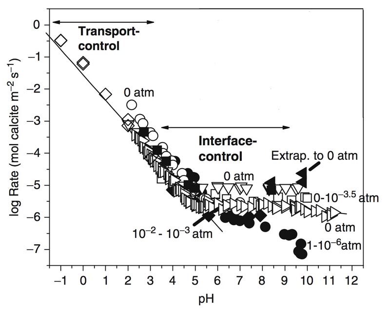
Generalized Transition State Theory (TST) Rate Law
A general TST rate law is as follows:
Here nk is the total number of parallel reactions, kj is the rate constant of the parallel reaction , the term describes the rate dependence on pH, and the term describes the rate dependence on other aqueous species that potentially accelerate or limit reactions. In Equation (4) for calcite dissolution rates, also accelerates calcite dissolution. The affinity term quantifies the distance of solution from the equilibrium state of the mineral reaction j. The exponents m1,j and m2,j describe the nonlinear rate dependency on the affinity term and are normally measured in experiments. Note that Equation (4) is a special case of the general reaction rate law in Equation (5).
Various factors affect reaction rates, including, for example, temperature, salinity, pH, organic ligands. Mineral dissolution rates are often accelerated by the presence of H+ or OH-. As a result, many minerals dissolve fast in acidic and alkaline conditions and slow down under neutral conditions. Figure 2 shows silicate dissolution rates as a function of pH.
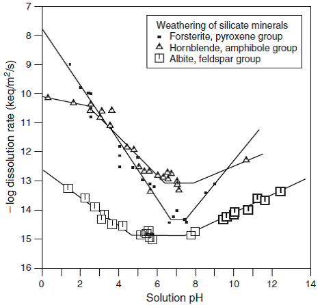
The intrinsic dissolution rates of minerals vary significantly. Calcite dissolution is in the fast end of dissolution rate spectrum, while quartz dissolves the slowest. Table 1 shows the lifetime of a 1mm crystal of different minerals, indicating more than 5 orders of magnitude difference in dissolution rates of silicates and quartz.
| Mineral | Lifetime |
|---|---|
| Quartz | 34,000,000 |
| Muscovite | 2,700,000 |
| Forsterite | 600,000 |
| K-feldspar | 520,000 |
| Albite | 80,000 |
| Enstatite | 8,800 |
| Diopside | 6,800 |
| Nepheline | 211 |
| Anorthite | 112 |
Rate Constant Dependence on Temperature
The Arrhenius equation is used to quantify the reaction rate dependence on temperature.
Here AF is the pre-exponential factor and is usually considered as a constant that is independent of temperature: the activation energy is always positive; here R is the ideal gas constant , T is the absolute temperature (K). If we take the logarithm of this equation, we obtain:
This means if we draw lnk versus , we get a straight line, as shown in Figure 2. For a particular reaction, if and at the temperature T1 is known, at another temperature T2 can be calculated by
Figure 3 shows the dependence of calcite rate constants on temperature under different CO2 partial pressure.
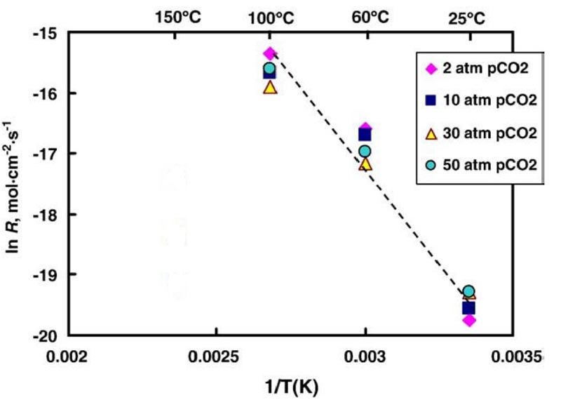
2.3 Set Up of mineral dissolution in a batch reactor in CrunchFlow
To model the mineral dissolution/precipitation, we need to inform the code both reaction thermodynamics and kinetics. Here we introduce how to set up simulations for mineral dissolution/precipitation in a well-mixed batch reactor, where the concentrations of all species and temperature are assumed to be spatially uniform. That is, the rate of mixing is faster than the rate of dissolution or precipitation, which is in general true for most minerals except carbonates under very low pH conditions. No transport processes and boundary conditions need to be defined because of the assumption of uniform concentration. The example 6 included in the CrunchFlow package is also a good reference for kinetic reaction setup.
Example 2.1: Calcite Dissolution
Calcite dissolution proceeds through three parallel pathways as shown in reactions (1)-(3). In addition, a series of fast aqueous complextion / speciation reactions occur simultaneously. These fast reactions are similar to those in the examples in the lesson on Aqueous Complexation.
In a batch reactor of 200 ml, the initial solution is at a pH of 5.0 with close to zero salinity. The initial total carbonate concentration is . The kinetic rate constant for three parallel reactions are , and respectively. The volume fraction of the calcite grains in the batch reactor is 0.5%, with a specific surface area (SSA) of 0.24 m2/g. Please set up the simulation and plot the following quantities as a function of time:
- Total Ca(II) and total inorganic carbon;
- Individual Ca-containing species and carbonate species;
- pH and the saturation index
Here is a light board video (12:44) of what equations the code solves for this system.
Mineral Dissolution & Precipitation
PRESENTER: So in this video we're going to talk about mineral dissolution and precipitation, the equation involved and interaction involved. This is different from the previous lesson, aqueous [INAUDIBLE], because the previous reaction only involved reaction [INAUDIBLE] dynamics. Meaning we care about the end point of the reaction.
When we have mineral dissolution precipitation, because reaction usually occur at the interface of solid phase and water, reaction occur much slower. So we often need to consider the kinetics of the reaction. Meaning we care about how long it takes for the reaction to occur to reach the end point.
So what I'm going to do today here is using the carbonate dissolution system in a battery reactor. So battery reactor, meaning it's closed while mixed, so that it does not have constitution gradient in different parts of reactor. So essentially you're solving for one constitution for each species for the whole reactor. So that's our systems.
If you think about if you want to draw something relevant to what you do in the lab, but you think about these water, and then you have these calcite grains, and you have these mixers that will keep the system well-mixed. And again, the reaction involving this system is similar to what we talked about last time for the aqueous speciation. The carbon and water-- for example, all these three reactions are the same as what I wrote before. Invest in one. But the key thing is we are adding this calcite dissolution, which is calcite dissolving out to become calcium and carbonate.
Calcite or carbonate in general is a very common type of rock or mineral fissure or surface. So it's a reaction. Compared to the aqueous speciation or [INAUDIBLE], it's much slower. But compared to other type of mineral dissolution, it's actually reactive fast.
So we have these four reactions here. You can think about the calcite dissolution essentially kind of releasing out the elements from the solid phase the water phase. So it dissolve as an add to the water with calcium species and carbonate species. But then once carbonate is released into water, it quickly goes through the speciation reaction to become either bicarbonate or carbonic acid, depending on the pH a system, as we talked about last time.
So if you think about the species in this system, now that the species we have, in addition to the five species, carbonic acid, bicarbonate, carbonate-- this is wrong. So it should be carbonate. And this should be two.
So you have these three carbonate species. You have hydrogen ion, which minus acid five, as before. But on top of that, you are adding calcium.
So essentially, now you have six species. You would have Ca2 plus carbonic acid carbonate, bicarbonate carbonate. And then you also have H plus or H minus. So that's six species.
So what does that mean, is that we essentially have six unknowns to solve for. And we will need six equations to solve for this, to solve for the species. But notice that one things that we need to pay attention to is that we have these three reactions that occur fast.
So you have these three equations already there. We can think about as one, two, three. That is as a three relationship. But we cannot use this one, because this is not a faster reaction. These are fast reaction.
This is a slow reaction, which means we need to care about its kinetics. Like how far it release as these chemical species over time. So when we solve these equations, we actually need to consider these time component.
In this case, we will need to think about the mass balance of system. So these calcite dissolving out and release out. For example, Ca2 plus, and releasing out CO3 bicarbonate. And then this will be exchanged into bicarbonate and exchange into carbonic acid. So these three specie are exchangeable.
So when we think about mass balance of system, you would think about the constitution of a single body calcium first. Volume-- this is a volume of the water in the system. And you have the constitution of calcium.
Ultimately, we are solving for contrition, not activity. So this will give you the mass. So contrition of the unit and mass per volume. And then we will need to solve for order and differential equation now because just time component here. So in this kind of system we don't really have fro transport so the only source of zinc of this calcium specie is through these reactions.
So let's say we have a rate constant of this reaction is Ksp. So that's the rate constant. And we talk about the tst rate, which is transition state rate theory in the online material. So you can go look this up.
So this Ksp and this is rate constant times a surface area of the mineral. And then times for example, how far away the reaction is from equilibrium, which will depends on the activity of Ca2 plus activity of carbonate, and then divided by Ksp, which is how far away this is from equilibrium. So this is Iap.
Now when we have dilute system-- if we have dilute system, then this activity would be equal to c. So you can replace every a is c for simplicity. So essentially, is this equation saying mass of calcium is added to system, to the water, by having this rate lower for calcium. But we also will have adding total carbon to the system. So similarly, you will have V, d, and then we call it total carbon cT, dt.
It will have the same expression here as Ksp A or minus activity ca. Because, essentially, it's through the same reaction. So this rack essentially adding calcium total carbonate-- this CT will be equals to again, constitution of carbonic acid plus concentration of bicarbonate and concentration of carbonate.
But then we need one more equation. One, two, three. And then this is four, this is five. We need a six equation, which would it be-- if you think about it, when this mineral dissolving out to form calcium and carbonate, it's actually changing the pH of the system. So the hydrogen ion-- or somehow we also call it's a measure of acidity of system will also change.
I'm not going through the detailed derivation of the whole process how we come up with. But let's call this dC, which is-- so this a constitutional cT-- concentration of hydrogen ion total dt. And by dissolving out calcite, actually decrease acidity of system. So it will actually have minus Ksp. And then activity one minus a Ca2 plus.
So again, it's the same rate law, but it do actually have the minus signs. That meaning it's decreasing the total acidity of a system. So the expression for the total acidity will be different if we define different to comnination primer specie.
But in general, if we define this carbonate as a primary species, we should have HT equal to hydrogen, concentration hydrogen ion. This should be CHt. Hydrogen ion plus concentration of H2CO3 minus concentration of bicarbonate and minus concentration of OH minus. You can actually derive this equation from the [INAUDIBLE] method. And these expressions is actually-- you can look at [INAUDIBLE] And by combining different terms, you come up with this. So essentially, we have six unknowns, and you have six equation to solve with that. But on top of that, one thing we need to pay attention is that these are OD equations.
So we call it ordinary differential equation. Differential equation, meaning we have one independent variable, which is time in this equation. So typically, the code will be solving these equation first using time stepping.
And then once we get the concentration calcium, concentration of CT, concentration of CHt, you have three kind of variable in particular time step. And then we solve for the algebraic and relationship with these numbers together with these three relationship. And by doing that, we essentially get the concentration of all the six species as a function time in these aqueous species. And what do you see? For example, your homework is essentially generated by solving these equations.
Here is a video demo in CrunchFlow on how to set up the simulation in CunchFlow (43:51 minutes).
Li Li: OK, so let's start. This is lesson 2 on mineral dissolution and precipitation. Now, with example 1, it's to set up as if you are doing a batch reactor experiment with some calcite grains in the solution. And you essentially will be running numerical experiments, imagining that your calcite dissolution rates are in these given numbers-- you have how much calcite grain in the system, et cetera.
So here-- let's see. For this lesson, the difference between this one and previous one in lesson 1 is, lesson 1 only have aqueous complexation. So it doesn't have any kinetics, it only has thermodynamics. The other one is zero-space dimensioning, and also, no-time dimensioning.
Now here, by introducing the reaction kinetics, we are essentially now looking at it as a time dimension. We'll still have a well-mixed system, which is a zero-dimensional system. We're not looking at things change in the functional space, so you have uniform contusion in the batch reactor.
So that's a major difference. Let's read the example question, and then I would explain a little bit, and we can try to set it up in CrunchFlow. OK, so example 1 is about a calcite dissolution. Calcite dissolution proceeds through parallel pathways, as shown in reaction 1 to 3. That's what we have-- we're seeing lesson 2.
In addition to these kinetic reactions, there are also a series of instantaneous aqueous complexation reactions, that occur at the same time. The three fast reactions should be the same as the ones in the example 2 of lesson 1. Also, that's for these fast reactions on the aqueous speciation reaction. So this essentially specify what aqueous speciation reaction you should include in this example.
Now, in a batch reactor, the initial solution is at a pH 5.0, with close to 0 salinity, meaning it is not a constituted solution. The initial total carbon concentration is 3.15 times 10 to the minus 4 mole per kilogram water. Kinetic rate constant for three parallel reactions are 1.00 times to 10 to the minus 2, 5.62 times 10 to the minus 6. And then the other number-- this is for the corresponding three reactions in 1, 2, 3.
And then the volume fraction of the calcite grains in the batch reactor is 0.5%. So if you have 100 milliliter, then you have 0.5 milliliter of calcite. You can convert that to how much mass is this with a specific surface area of 0.25 meters squared per gram. Please set up the simulation and plot the following quantities as a function of time.
So now we're looking at the time dimension, right? We're starting from the initial condition. So initially, you have some total carbon concentration there-- 3.15 times 10 to the minus 4 mole per kilogram. But essentially there, you don't have other species.
Now, the question it's asking you, first of all-- so total calcium concentration and total inorganic carbon. So you need to plot that as a function of time. Second was the individual calcium-containing species. And carbon is species. And so here, you want to see, essentially asking, which one the dominant species and everything. And then also, the pH and IAP over Keq, which is a saturation index. Maybe that-- make it more explicit.
OK, so let's do this. Let's go to that folder again. OK, again-- so I have four files here waiting for you. Let's open the input file. Oh, I hate it when-- let's do it in Notepad. I don't like all these red line and everything-- underlining all my words. Let's open it with Notepad. OK. Much better.
All right, so this is a template, essentially. And we need to fill in, OK? So this did not say TITLE will be "lesson 2-- calcite dissolution in a batch reactor." These runtime specifications are still there. Database-- make sure it's datacom.dbs and everything. OK.
So here, make sure you don't do speciate only, because when you do speciate only, the time is not going to be stamped, and you cannot do this calculation. Because this is for kinetic, and you want your time stamping Output file-- the output procure block. We need to specify what we want the system to output.
So first of all, we need to specify, what units are we using? Let's do seconds. We know calcite dissolution very fast-- or maybe minutes. Let's do minutes. And let's call it time. We need to specify time series. And let's call that calcite dissolution .out.
And for batch reactor, we should only have one group block. So let's just specify this as a group block 1. Time series print. So what time series print do is, you specify what species you want to print. So you can put a specific freedom-- calcium.
And this need to be the-- I'm just going to make it explain. Needs to be primary species. It cannot output times there for secondary species. So we can specify it's the calcium pH or bicarbonate. But it's very important that maybe we'll do all-- "all" meaning all primary species would be printed out.
Discretization-- we should only have one species, right? So first, we need to specify the units' distance-- units. Let's say it's meters. And then, when you need to specify kind of zones-- x-zones, y-zones. So you have x-zones should be 1.1. So you only have one group block.
Now, for the other dimensions-- if you only specify 1, so that essentially you have 1 meter, 1 meter, 1 meter. If you don't specify other, it will assume it's meter-- the same units-- and it's 1. Quantity is 1. So essentially, you have 1 meter cubed. Maybe we'll make it centimeters, just to be more realistic.
And you have 10.0. It shouldn't matter, because we are specifying volume fractioning, not a specific number. And so if I'm specifying-- maybe I will do 100. Because a typical batch or a flux or something, that you would do batch reacting as hundreds of milliliters. So I'm specifying here-- this is 200 centimeter cubed, essentially. The other two dimension-- y-direction and z-direction into it-- by default, it will be 1 centimeter, 1 centimeter. So it should be 200 centimeter cubed-- essentially 200 milliliter. That's the discretization.
Now, we actually also need-- in output, we need to specify how long we want this to run-- spatial profile. So maybe we'll do, let's say, 1 minute. And then, maybe 20 minutes? 10 minutes. OK. Maybe 10 minutes. It is out pretty fast. Let's see. It's 5.0, 10.0, 50.0. All right. So we run it for 100 minutes. So it's the end point time. So this submission would be run until 100 minutes.
Now, we don't have spatial discretization. We don't have. We only have one group block. It's a well-mixed system, so we don't need to specify-- we don't have something coming from the boundary. We should be fine. So let's specify-- initial conditions should be whatever condition we specified it. So let's do it later.
We don't have transport. We can safely delete that. We also don't have flow, we don't have porosity. We can now delete all of that. So the primary species you want to put in, we talked about before. You should have calcium. First of all, all we need-- H plus, actually. What else you need? I'm going to look at the question again.
Let's put a bit of sodium chloride there, just in case we need-- to make charge balanced, we can use sodium chloride. So usually, you use species that are not reactive to do charge balance. Otherwise, you would be changing the condition we put in the species.
What else? And we need bicarbonate speciates-- still use bicarbonate. That should be it for primary species. Second species-- again, OH minus would be the top one. Or the other carbonate species-- A, Q-- 0 3. Potentially with these, we could form COH plus-- that's another aqueous species.
You can check by doing speciation only-- by data sweeping or something-- to see which species will be dominating, if you would like. But that's your calcium. Carbon we also form-- aqueous calcium carbonate. And if you would have carbide, possibly you would also have that. OK, I think that's good for our second speciate, I believe.
OK. So for this one, we need initial condition. Because the system started with-- this is where t equal to 0. So let's call that condition initial. And you will need all the prime-- you need to specify all the primary species, so copy the list of primary species here.
So question says, initial pH is 5.0. So let's specify pH would be 5.0 first, instead of saying H plus. Let's do 5.0. So initial calcium concentration should be almost 0. Now usually, I try not to put directly zeroes there, because sometimes computers have problem with 0. And I always put a very small number there, just in case. So for the very small-- essentially none-- I'm putting very-- these 10 to minus 10 concentrations. All right.
Bicarbonate is a good-- the question said, initially, it's 3.15 times 10 to minus 4. OK, they say what you put in there. That's the total concentration saturate, not specific. And question says, total carbonate concentration. That's consistent.
Now here, we also have either-- in solution, we should also have calcite, because calcite need to dissolve out. So we need to have the calcite mineral. This is very important, because otherwise, there would be no representation calcite going in there. So let's put calcite. And it says, volume fraction is 0.05%.
So the first number should be the volume fractioning. And then, it also says, specific surface-- the key word is specific-- surface area is 0.25. So let me just comment on that. The first number, volume fractioning, is 0.05. This SSA is 0.24 meter squared per gram. So that's the unit.
You can also specify total surface area, I believe. Let me just search the manual. I believe you can do-- this should be similar. Oh, you can specify BICG surface area or specific surface area. If it's BICG surface, you'll be putting the absolute value. If it's specific surface area, it should be in the units meter squared per gram.
So it's the typical-- the way you're putting is, name of solid face, volume fractioning, surface area option, and value. BICG surface area. So you can look through these if you would like to have more details. Go into page 68, 69 in the manual. All right.
Now, we cannot put in the grain size. But the specific surface is more or less refracting the grain size you have. When you have small grains, you tend to have larger specific surface area. And when you have larger grain, you have small specific surface area. But also, of course, for different mineral, they're also different. OK. So the initial condition.
But one thing we're keeping-- we need to keep in mind is that the solid face need to be recognized by the mineral-- key word, block. This is where you're putting the kinetic information. Without that, you will either use the kinetic information grid block, or in the database-- which I usually prefer to putting input file, because then you have everything in the same place.
So here, you will need to put in the rate constants in the log 10 units. These rates should be in log 10 rates in units of mole per meter squared per second. All right? So the way you're putting is calcite, and then you have the label, if it splits it using default.
Then your rate is-- OK. Let me just check the three reaction pathways. We are saying, for calcite, you have these three reactions. So you have k1, k2, and k3. They all have the same-- so one is, k1 depends on each process. k2 depends on H2O CO3. k3-- there's no dependence. So let's just also check the database.
Let's save it, and let's look at database. Make sure it's a default in everything. Make sure we know what are the format for each label. Search for calcite. OK. So this said, T-S-T rates are-- default is-- OK. H plus 1 is one that depends on each process. That's the k1, right? So let's see, label. So you need to look back and forth a bit. So let's do H plus first.
And I said, the rate constant is what? 1 times 10 to minus 2, for the 3 or 4 k one. OK, for the H plus dependence once. So this one is-- in units of mole per meter squared per second. So this one should be minus 2. And then, you have the-- so second one is-- let's call it a CO2, so it's less confusing. Let's call it a CO2 dependence. And it's dependent on this with 1.0.
So this dependence need to specified in the database, but not the one-- so I probably should say H2O3. And then, the default is 1 without any dependence. OK, so if we specify the number here-- OK, so that will be CO2. And then rate.
So the second rate constant is 5.62 times 10 to the minus 6 in log unit. Let me just-- 5.62. OK, 10 to the minus 6-- minus 6. So it's 5.25. All right. And then, the default ones without dependence is 7.24 times 10 to the minus-- so 7 point. Minus 9-- minus 8.14. For the three parallel reactions-- 1, 2, and 3. OK.
So now, what-- so these rate constants should be override to whatever that is in the database. OK, you have condition-- let's just check it. You have a condition-- you have mineral specified with kinetics. You have primary and second species. OK, you need to specify what are the initial condition.
So you should have say, initial condition-- initial, we call it-- yeah. We called that initial. So this condition will be in the first code block. We only have one group block. This is specify the location and-- you can dig into manual for them-- search for this key word block, and the manual explain in detail what you can put in.
So here-- this initial condition is interesting. OK, I'm using this initial condition for this group block 1. Let's see if they run. I think you should. And so I made a mistake somewhere. So that's 2 lesson, example 1. Oh-- rate label. Cannot have enough on-- in database. Looking for calcite rate label CO2. Let's see. Hm. Interesting. Maybe I didn't save it.
OK, let's do it again and just save it 2 lesson example. Now it runs. There's something else coming up. So the other time I changed it, the to CO2, but I didn't save it. So the code doesn't recognize the CO2 label. So I save it to the database with the CO2. Then the code not recognize that label.
And then, now is speciation-- OK. So it-- speciation is finished. No aqueous kinetic block found. Retardation parameters not found. Both the number of cells and the grid block spacing should be-- oh, OK. Only one value provided. Yeah, I've seen the problem with discretization. So I need to provide-- let's go to-- just make sure we-- discretization key word block-- x-zone, y-zone, z-zone.
OK. At discretization, you can specify x-zone, z-zone, y-zone. So the syntax is-- it's supposed to say x-zone. And it's how many number of cells and spacing. OK, good. And number of cells should be integer, and spacing is a real number. So we are saying, we have one group block. And the spacing is-- it's 200 centimeter. I think that should make it work. Let's try it again. So I just look it up and do it again.
All right. So the runs is finished. That's good. OK. And suddenly, you discover there are a lot of output files. Each of these output file-- for each of these-- these are all out, right? So you have each of these every time. You have every 1, every 2, every 3, 4, 5. Each of these is corresponding to one of these times that you specified in the spatial profile. Remember, in spatial profile, I put 1 minute.
So it's spit out the output at 1 minutes, 5 minutes, 10 minutes, 50 minutes, and 100 minutes. So the 1 will be representing 1 minutes. 2 will be 5 in this. So each of these have 5. Right? I said 2, perhaps there is 5. Concentration have 5. Guess mineral percentage, because you have mineral. pH, porosity-- a lot of information.
OK, these are standard operations. Some of them are not useful for this example. But I want to-- let's go through. So you don't have to answer questions at these. You want to print-- plot everything in the function of time. All these other areas-- like, area 1 to 5-- because we only have one grid block. So the spatial profile is not really useful for us.
If we have 100 grid block, we want to see how this varies spatial rate. Now you only have one grid block. So it's not really interesting. It's more interesting to look at that as a function of time. And then we specified the breakthrough curve should be in-- OK. Calcite dissolution data out. So let's look at that file. This will be what you should look for for the breakthrough.
Calcite. This-- OK, this good. So as we said, essentially output everything, right? OK. So again, first it's time stepping varied with very tiny time steps. And then, later, it becomes more larger times then, because it's approaching to equilibrium.
Now look, and so you have pH, you have H plus, calcium, sodium chloride, always a function of time. We said "all," so it also spit out sodium chloride. But we actually don't really need that. But why-- OK, we also should have-- OK. Hm, interesting. Bicarbonate, H plus, CO2, AQ, 03, calcium. So it actually does spit out all the aqueous speciation, as well.
And these are inactive variables. These are in, actually, log units. For the primary species, it's an absolute value. It's not log. For the second species there, you log in log. So this, it would be 10 to the minus 8.99, 10 to the minus 3.52, 10 to minus 9.5, for example. So they should be increasing.
So you actually can directly read, if you want, to plotting. So you can either do Matlab, Excel, whichever ways are the easiest for you. Let me just show you how to open that in Excel, so if that's easiest for you. I'm opening up Excel. And I will say, Open. Hm. Why don't you-- oh. It's says no book. Sorry.
OK, let's do this one-- let's see how. OK. So you would say, so the code, I can actually fix the widths. It will space out for this. OK, it probably doesn't matter. OK, so you have all the different species-- pH, H plus, pH. So you can plot-- whichever that I asked for you can plot. Problem is species. Pay attention, there's this thing.
OK, so this also give the calcium in the log units. So these are individual species, and these are the total for the primary species. So if you want to plot a primary species, like the individual species, you do want to use these columns, starting from H plus here, when it has a log-- after it's already been log.
So this is how you can do, for example, getting all the time series and plot out the files. So that's an example. You can see all the change in the function of time, how the saturation changed the function of time. So here, I'm giving you the solution already, but you want to be able to generate that by yourself. I want to be able to see that.
And you shouldn't just-- before you do anything, you shouldn't look at this solution yet. But I'm still telling you, here-- these solutions, OK. For the individual concentrations, OK, these are total calcium, total bicarbonate. So it should be from the first several columns on primary species.
And you can see, the carbon is always higher than the calcium, because initially, there is some carbon in species there. So if you look carefully, the difference is actually exactly the initial concentration of carbonate. Because essentially, the calcium-- when the calcite dissolves, it should be dissolving calcium and total carbon in one-to-one stoichmetric coefficient.
When the calcite dissolves, pH increases over time, until it reach around 8, so it's concentration in which certain values stopped, because it reach equilibrium. IAP over Keq get to about 1, which is at equilibrium at about 120 or 130 minutes, which is similar to where concentration reached a plateau.
And looking at the individual concentrations-- so this is a bit hard to see. Total calcium should be the highest, and blue is-- so the free calcium is a dominant species. And then this light blue, you see it-- bicarbonate. So calcium bicarbonate is the second one. Red one is Ca CO3, and then you have COH plus, which is reasonable, because you have a lot of carbonate species in the system.
So that should give you a sense of how you would do with the mineral dissolution precipitation. And as an extension of the example 1, in the homework assignment, I asked you to do the carbon dissolution, changing several key parameters, essentially.
Example 1 did all this in one particular condition. But we all know, in the lessons, we discussed where the constant is important, surface area is important. Initial pH, salinity-- all these things are important. So how do they change the dissolution process, if we change these numbers? So in every question of these, it asks you to change your numbers, and compare three different cases, in term of how things are different with different sets of parameters.
And then, the question 1 is about feldspar dissolution. So in example 1, give you everything about calcite. In question 2, you are supposed to calculate to set a feldspar dissolution using the figure 7 in Blum and Stillings, with the rate dependence on H plus, OH minus, or the neutral one without any pH dependence. And you should be able to study that up to run these simulations.
All right, I think I'm going to stop here. And I hope you have fun playing with CrunchFlow in setting up mineral dissolution precipitation. Again, this is in batch reactor. So imagine that you are doing a numerical experiment of the batch reactor, and you're putting calcite grains-- different grain size.
So you have larger, smaller specific surface area, and all that. OK, I'm going to stop by, and hope you have fun here. And we can discuss later, if you have questions. OK.
Figure 4 below shows the evolution of aqueous chemistry during calcite dissolution. Total Ca(II) and carbonate increases over time and should follow the 1:1 stoichiometric ratio. However, total carbonate concentration is higher due to the initial presence of total carbonate at the concentration of . The individual speciation of Ca(II)-containing species are in D shows that Ca2+ is the dominant species. During the dissolution, pH and increase over time, until reaching close to 1 at about 100 minutes, after which the system stabilizes and no more dissolution occurred after that.
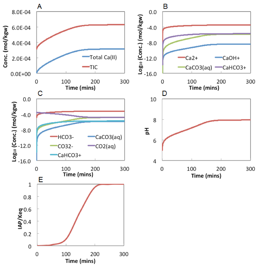
As can be seen from these figures, the dissolution reactions reach equilibrium at about 200 minutes, where pH increases to about 8. Total Ca(II) include Ca2+, CaOH+, CaCo3(aq), and CaHCO3+, with Ca2+ being the dominant species (shown in figure 4B). Total inorganic carbon includes CO2 (aq), HCO3-, CO3--, CaHCO3-, and CaCO3(aq). HCO3- is the dominant species at most of the time except very early time when pH is still at about 5, where CO2(aq) dominates.
2.4 Homework Assignment
1. Carbonate Dissolution (Example 1 extension) (Total 70 points, each sub question is 10 points):
Thermodynamics and kinetic parameters that affect mineral dissolution include specific surface area (SSA), kinetic rate constants (k), and equilibrium constants. In addition, geochemical conditions can also have a large impact on mineral dissolution rates, including salinity (e.g. NaCl) and pH. With the provided CrunchFlow template files in example 1 as a starting point, please do the following analysis comparing Ca(II) concentration evolution under different parameters and geochemical conditions. In each question, please only change the parameter that is discussed and keep all other parameters the same as those in Example 1.
1) Calcite specific surface area (SSA). In three different simulations, run the code using SSA being 0.024, 0.24, and 2.4 m2/g. Plot the total Ca(II) as a function of time under these surface area values in one figure. Discuss how SSA affects calcite dissolution kinetics.
2) Kinetic rate constant: increase and decrease the original three rate constant values in Example 1 by an order of magnitude. Compare the Ca(II) concentration evolution under the three k values in one figure. Also compare this figure here with the figure in 1) with the SSA of 0.24 m2/g. Do changing k and A have the same impact on dissolution rates?
3) Equilibrium constant Keq quantifies how much a mineral can dissolve in aqueous phase. Increase and decrease the equilibrium constant by an order of magnitude. Please plot the three curves (total Ca(II) ~ t) with different Keq values in one figure. What do the rate kinetics change with the total Ca(II) evolution figure?
4) Initial pH condition. Compare the base case with two more cases where you have the initial pH being 4.0 and 6.0.
5) The role of speciation. In this question you remove all secondary species such as CaOH+, CaCO3(aq), and CaHCO3+. Draw the same figures as those in Example 1 and solution from this question if the same figure. Compare and describe your observations. Does the reaction system evolve in the same way in these two systems? What do you think are the effects of speciation?
6) Salinity: in the base case scenario there is no NaCl in the solution. Simulate two more cases with NaCl at concentrations of 0.01 and 0.1 mol/kgw, respectively. Please compare total Ca(II) evolution under these three salinity conditions.
7) Go back to your answer to each question 1)-6). Summarize your observations in these questions. Which factors have the most significant control on calcite dissolution?
2. Feldspar Dissolution (optional, bonus points: 30, for students who develop clear solution and reasoning):
Feldspars dissolve following the TST rate law and have very different dissolution rates depending on their composition (figure 7 in [Blum and Stillings, 1995]). Pick a feldspar mineral from the paper and/or the cited reference that has a complete TST rate law from acidic to alkaline conditions. Set it up in CrunchFlow to simulate its dissolution with initial pH conditions varying from acidic (for example, pH =4.0), to neutral (pH = 7), and to alkaline condition (pH = 10.0). Compare the reaction production evolution under these three conditions. Please make sure that you use reasonable rate constant and specific surface area values from literature.
2.5 Summary and Final Tasks
Summary
In this lesson, we learned about mineral dissolution and precipitation reactions. We discussed two aspects of the reactions: 1) reaction thermodynamics that control how much minerals can dissolve in aqueous solutions; 2) mineral reaction kinetics (TST rate law) and parameters that control the rates of mineral dissolution and precipitation. We also learned how to set up running simulations in CrunchFlow for mineral dissolution in well-mixed reactors.
Reminder - Complete all of the Lesson 2 tasks!
You have reached the end of Lesson 2! Double-check the to-do list on the Lesson 2 Overview page to make sure you have completed all of the activities listed there before you begin Lesson 3.
Homework assignments for lesson 2 is due on Tuesday before midnight.
References
Appelo, C. A. J., and D. Pstma (2005), Geochemistry, groundwater, and pollution, 2nd ed., 649 pp., CRC Press, Taylor and Francis group, Boca Raton, FL.
Blum, A. E., and L. L. Stillings (1995), Feldspar dissolution kinetics, in Chemical Weathering Rates of Silicate Minerals, edited by A. F. White and S. L. Brantley, pp. 291-351, Mineralogical Soc America, Washington, D. C.
Brantley, S. L. (2008), Kinetics of mineral dissolution, in Kinetics of water-rock interaction, edited, pp. 151-210, Springer.
Chou, L., R. M. Garrels, and R. Wollast (1989), Comparative study of the kinetics and mechanisms of dissolution of carbonate minerals, Chem Geol, 78(3), 269-282.
Lasaga, A. C. (1984), Chemical kinetics of water-rock interactions, Journal of Geophysical Research, 89(B6), 4009-4025.
Plummer, L., T. Wigley, and D. Parkhurst (1978), The kinetics of calcite dissolution in CO 2-water systems at 5 degrees to 60 degrees C and 0.0 to 1.0 atm CO 2, Am J Sci, 278(2), 179-216.
Pokrovsky, O. S., S. V. Golubev, J. Schott, and A. Castillo (2009), Calcite, dolomite and magnesite dissolution kinetics in aqueous solutions at acid to ciarcumneutral pH, 25 to 150° C and 1 to 55 atm p CO2: New constraints on CO2 sequestration in sedimentary basins, Chem Geol, 265(1), 20-32.
Lesson 3: Surface Complexation
Overview
This lesson introduces general principles of surface complexation reactions, as well as how to set up surface complexation models in well-mixed batch reactors in CrunchFlow.
Learning Outcomes
By the end of this lesson, you should be able to:
- Understand what are surface complexation reactions;
- Comprehend thermodynamic controls of and important parameters for surface complexation.
- Simulate surface complexation reactions in well-mixed batch reactors in CrunchFlow
Lesson Roadmap
| To Read |
|
|---|---|
| To Do |
|
Questions?
If you have any questions, please post them to our Questions? discussion forum (not e-mail), located in Canvas. The TA and I will check that discussion forum daily to respond. While you are there, feel free to post your own responses if you, too, are able to help out a classmate.
3.1 Background
Sorption is the adhesion of chemicals to solid surfaces. Adsorption process occurs in many natural and engineered systems. Studies of contaminated systems have shown that sorption–desorption is an important geochemical process that regulates transport and fate of inorganic and organic contaminants in natural subsurface systems. For example, metals (Cd2+, Cr3+, Co2+, Cu2+, Fe3+, Pb2+ or Zn2+) can become immobilized by sorbing on sediments and soils. They can also become mobilized through desorption from the solid surface and re-enter the aqueous phase when geochemical conditions allow. Sorption-desorption is widely used in industrial applications including charcoal activation, air conditioning, water purification, among others.
Sorption can occur either specifically or non-specifically as shown in Figure 1. Chemical sorption (Specific adsorption) is highly selective and occurs only between certain adsorptive and adsorbent species. A chemical bond involves sharing of electrons between the adsorbate and adsorbent and may be regarded as the formation of inner-sphere surface complexes. Chemical adsorption is difficult to reverse because of the strength of the formed bond. Physical adsorption (nonspecific adsorption). A physical attraction resulting from nonspecific, relatively weak Van der Waal's forces. Being only weakly bound, physical adsorption is easily reversed. Multiple layers form through outer-sphere surface complexes during physical adsorption [Goldberg 1991; Webb, 2003].
Sorption via surface complexation has been extensively studied. Surface complexation is the process where species in the aqueous phase form complexes with functional groups on solid surfaces, similar to aqueous complexation in lesson 1. Surface complexation function occurs between aqueous species and functional groups on solid surface, instead of the formation of complexes between aqueous species in aqueous complexation reactions. Surface complexation models use mass action laws that are analogous to aqueous geochemical conditions and solid phase properties.
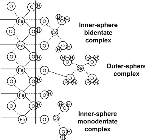
3.2 Surface Complexation Models (SCMs)
Surface complexation models describe sorption based on surface reaction equilibrium. Similar to aqueous complexation, surface complexation reactions are considered fast reactions and are controlled by reaction thermodynamics.
Surface Configuration of the Solid–Solution Interface
There are three commonly used SCMs, the constant capacitance model (CCM), the diffuse layer model (DLM), and the triple layer model (TLM). These models differ in complexity from the simplest CCM that has three adjustable model parameters, to the most complex TLM that has seven adjustable parameters [Hayes et al., 1991]. The double layers exist in practically all heterogeneous fluid-based systems. Here we introduce the principle and thermodynamics of DLM.
The double layer refers to two parallel layers of charge surrounding the solid surface. The first layer, the surface charge (either positive or negative), comprises ions sorbed onto the solid due to chemical interactions. The second layer (“diffuse” layer) is composed of counter ions attracted to the surface charges via the coulomb force, electrically screening the first layer. The schematic of double layer is shown in Figure 2.
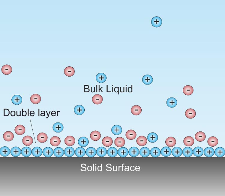
Surface Complexation Reactions
In traditional SCM models, all reactions are considered as at equilibrium. As an example, the surface protolysis reactions, where H+ transfers among chemicals, are given by:
Here the $\equiv S O H$ represents a species or functional group on solid surface. In the first reaction, $\equiv S O H$ gains an H+ and becomes positively charged. In the second reaction, $\equiv S O H$ loses an H+ and becomes negatively charged. The apparent equilibrium constants Kapp describe the relationship between activities of different species, written in the same format as we do for aqueous complexations except now we include activities of solid species.
Similarly, for a metal ion M with a positive charge m, the reactions are represented by:
For an anionic ligand L with a negative charge of l, the reactions are represented by:
In these reactions, $\equiv S O H$ represents a surface site for the sorbent functional group, $\equiv S O H_{2}^{+}, \equiv S O^{-}, \equiv S O M^{(\mathrm{m}-1)}, \equiv(S O)_{2} M^{(\mathrm{m}-2)}, \equiv S O H_{2}^{+}-L^{l-} \text { and } \equiv S O H_{2}^{+}-L H^{(l-1)-}$ are surface complexes, [ ] represents the activity of each species or surface complex, $Mm+$ represents a metal ion of charge m+ and Ll- represents an anionic ligand of charge l−.
Apparent (Kapp) and Intrinsic (Kintr) Equilibrium Constants
The apparent equilibrium constant of surface complexation reactions, Kapp, is an important parameter because it determines the ion partition between aqueous and solid phases. Large Kapp values indicate high affinity of the ions to the solid surface. The relationship between total Gibbs free energy $\Delta G_{\text {tot }}$ and Kapp is as follows:
Here the total Gibbs free energy $\Delta G_{\text {tot }}$ can be further expressed as follows:
Here $\Delta G_{c h e m}^{0}$ is the intrinsic free energy of the chemical reactions at the surface; $\Delta G_{\text {coul }}^{0}$ is the electrostatic or Coulombic term that accounts for the electrostatic interactions:
Here Z is the charge of the ion, F is the Faraday constant (96485 C/mol), $\psi_{0}$ is the average potential of the surface plane (V). Therefore,
Where $K^{\mathrm{int} r}=\exp \left(-\frac{\Delta G_{c h e m}^{0}}{R T}\right)$, R is ideal gas constant $(1.987 \mathrm{cal} /(\mathrm{mol} \cdot \mathrm{K}))$; T is the absolute temperature (K). Take equation (1) as an example,
Where $K_{1}^{\mathrm{int} r}=\frac{\left[\equiv \mathrm{SOH}_{2}^{+}\right]}{[\equiv \mathrm{SOH}]\left[\mathrm{H}_{s}^{+}\right]}$ , Z is the charge of the ion (1 in the case of H+); $\left[H_{s}^{+}\right]$ is H+ activity on the solid surface.
The electrostatic or coulombic effect can be quantified as:
From equation (10), we know that $K_{1}^{\text {int } r}$ and $\psi_{0}$ are needed in order to calculate $K_{1}^{a p p}$. The $K_{1}^{\text {int } r}$ is typically estimated using zero charge extrapolation or using the double extrapolation method as discussed in literature. Under low ionic strength conditions where $\psi_{0} \cong 0$, the intrinsic and apparent constants are equivalent.
Surface sorption site
For different minerals, the number of surface sites differs significantly, depending on their surface properties. The abundance of surface sites is important in determining the total sorption capacity. The concentration of surface sites can be calculated as follows:
Here Csite is the concentration of surface sites (mol/g mineral), ρsites is the surface density of surface hydroxyl sites (mol/m2), Aspecific is the specific surface area (SSA)(m2/g). This equation says that surface site concentration depends on the surface site density and specific surface area. Please note that if you are working with porous media, you will need to calculate the total gram of minerals for surface complexation to get the total number of available sites.
Specific surface area (SSA) and site density values can be determined experimentally from Brunauer -Emmett-Teller (BET) surface area and tritium exchange measurements, respectively. The units of site/nm is often used in literature, where 1 site/nm = 1.66x10⁻⁶ mol/m2. Typical values of specific surface area (SSA) and site densities for different types of minerals are listed in Table 1. The total number of surface sites for a particular system (mol) can be calculated by multiplying site density (mol/m2) with SSA (m2/g) and the mineral mass (g). Minerals such as clays tend to have a large surface area and have a large capacity to sorb chemicals.
| Absorbent | SAA (m2/g) | Site density (mol/m2) Strong Site |
Site density (mol/m2) Weak Site |
Reference |
|---|---|---|---|---|
| Goethite | 14.7 | 1.76×10⁻⁶ | 3.22×10⁻⁶ | (Müller and Sigg, 1992) |
| Kaolinite | 19.5 | 2.20x10⁻⁶ | 3.00×10⁻⁶ | (Lackovic et al., 2003) |
| Illite | 66.8 | 1.30x10⁻⁶ | 2.27x10⁻⁶ | (Gu and Evans, 2007) |
| Smectite | 56.4 | 4.77x10⁻⁸ | 9.54x10⁻⁷ | (Bradbury and Baeyens, 2005) |
Different types of surface sites
Organic and inorganic chemicals are usually sorbed at hydroxyl surface functional groups that are located at the broken bonds and edge sites on minerals with excess negative charges [Baeyens and Bradbury, 1997]. We often classify two kinds of sorption sites: "strong" sites $\left(\equiv \mathrm{S}^{\mathrm{S}} \mathrm{OH}\right)$ and "weak" sites$\left(\equiv \mathrm{S}^{\mathrm{W}} \mathrm{OH}\right)$. "Strong" sites have a low capacity and a high sorption affinity and dominate the uptake of adsorbate at low concentrations. "Weak" sites have a considerably larger capacity however much lower sorption affinity. Table 2 shows reactions and equilibrium constants for U(VI) sorption on ferrihydrite, where FesOH represents strong site with orders of magnitude higher intrinsic equilibrium constants than those of the weak sites $\left(\equiv \mathrm{FE}^{\mathrm{W}} \mathrm{OH}\right)$ (Zheng et al., 2003). In this soil with the presence of ferryhdrate, the site density ratio of weak to strong site is 476:1 (i.e., 0.21% of the total surface sites, 99.79% for the weak sites).
| Reactions | LogKintr |
|---|---|
| $2 \equiv \mathrm{Fe}^{S} \mathrm{OH}+\mathrm{UO}_{2}^{2+} \Leftrightarrow \equiv\left(\mathrm{Fe}^{S} \mathrm{O}\right)_{2} \mathrm{UO}_{2}+2 H^{+}$ | -2.35 |
| $2 \equiv \mathrm{Fe}^{W} \mathrm{OH}+\mathrm{UO}_{2}^{2+} \Leftrightarrow \equiv\left(\mathrm{Fe}^{W} \mathrm{O}\right)_{2} \mathrm{UO}_{2}+2 H^{+}$ | -6.06 |
| $2 \equiv \mathrm{Fe}^{S} \mathrm{OH}+\mathrm{UO}_{2}^{2+}+\mathrm{CO}_{3}^{2-} \Leftrightarrow \equiv\left(\mathrm{Fe}^{S} \mathrm{O}\right)_{2} \mathrm{UO}_{2} \mathrm{CO}_{3}^{2-}+2 \mathrm{H}^{+}$ | 4.33 |
| $2 \equiv \mathrm{Fe}^{\mathrm{W}} \mathrm{OH}+\mathrm{UO}_{2}^{2+}+\mathrm{CO}_{3}^{2-} \Leftrightarrow \equiv\left(\mathrm{Fe}^{W} \mathrm{O}\right)_{2} \mathrm{UO}_{2} \mathrm{CO}_{3}^{2-}+2 H^{+}$ | -0.24 |
Surface charge and point of zero charge (PZC)
Surface complexation leads to surface-charged solid surfaces. Electric surface charges govern characteristic chemical and physical phenomena such as ion exchange, adsorption, swelling, colloidal stability, and flow behavior (Sposito, 1981). It is well known that the surface charges on layered silicates and insoluble oxides depend on the pH of aqueous solutions The pH of the point of zero charge (PZC), where the net total particle charge is zero, is a convenient reference for describing the pH dependence of surface charges. (Appel et al., 2003). When solution pH is above PZC, the solid surface has a negative charge and predominantly exhibits an ability to exchange cations, while the solid surface retains anions (electrostatically) if pH is below its PZC. A list of common substances and their associated PCZs is shown in Table 3.
| Chemical Formula | pHPZC |
|---|---|
| $\text { Kaolinite }$ | 4.6 |
| $\text { Montmorillonite }$ | < 2.5 |
| $\text { Corundum, } \alpha-\mathrm{Al}_{2} \mathrm{O}_{3}$ | 9.1 |
| $\gamma-\mathrm{Al}_{2} \mathrm{O}_{3}$ | 8.5 |
| $\text { alpha- } \mathrm{Al}(\mathrm{OH})_{3}$ | 5.0 |
| $\text { Hematite, } \alpha-\mathrm{Fe}_{2} \mathrm{O}_{3}$ | 8.5 |
| $\text { Goethite, } \alpha \text {-FeOOH }$ | 9.3 |
| $\text { Birnessite, } \delta-\mathrm{MnO}_{2}$ | 2.2 |
| $\mathrm{Fe}(\mathrm{OH})_{3}$ | 8.5 |
| $\text { Quartz, } \mathrm{SiO}_{2}$ | 2.9 |
| $\text { Calcite, } \mathrm{CaCO}_{3}$ | 9.5 |
3.3 Example 3.1
Cr(VI) sorption on illite in a batch reactor: Math formulation and CrunchFlow Setup
Example 3.1: Cr(VI) surface complexation on illite. Chromium is a common containment in natural subsurface due to its natural occurrence and wide industrial usage, including electroplating, pigmenting, and dye synthesis. Anionic Cr (VI) is highly mobile and poses a tremendous risk to human and ecosystem health. Clay minerals such as illite are important in controlling Cr(VI) sorption and natural attenuation due to its large surface area and ubiquitous presence (Wang and Li, 2015).
We have an initial solution listed in Table 4. The illite grains in the solution have specified surface area and site density of $\equiv \mathrm{SiOH}$. The surface site $\equiv \mathrm{SiOH}$ goes through several surface complexation reactions as listed in Table 4. Please calculate:
- At the pH = 8.0, calculate the concentrations of different surface complexes on the surface sites; what is the pH value after the system reaches equilibrium?
- If the initial pH is 4.0, calculate the concentration of different surface complexes on the surface sites; what is the pH value after the system reaches equilibrium?
| Initial conditions (total concentrations) | Value |
|---|---|
| Temperature | 25oC |
| Solution volume | 250 mL |
| pH | 8.0 |
| CrO42- | 9.61x10⁻⁵mol/L |
| Na+ | 0.01 mol/L |
| Cl- | 0.01 mol/L |
| K+ | 1.93x10⁻⁴mol/L |
| Al3+ | 1.00× 10⁻⁶ mol/L |
| Mg2+ | 1.00× 10⁻⁶mol/L |
| SiO2(aq) | 1.00× 10⁻⁵mol/L |
| Site density $\equiv \mathrm{SiOH}$ | 1.00× 10⁻⁶mol/L |
| Illite specific surface area | 15.36 m2/g |
| Illite volume fraction | 0.003 |
| Reactions | Log Kapp |
| $\equiv \mathrm{SiOH}+\mathrm{H}^{+} \Leftrightarrow \equiv \mathrm{SiOH}_{2}^{+}$ | 0.95 |
| $\equiv \mathrm{SiOH} \Leftrightarrow \mathrm{SiO}^{-}+\mathrm{H}^{+}$ | -6.59 |
| $\equiv \mathrm{SiOH}+\mathrm{Na}^{+} \Leftrightarrow \equiv \mathrm{SiONa}+\mathrm{H}^{+}$ | -6.60 |
| $\equiv \mathrm{SiOH}+\mathrm{CrO}_{4}^{2-}+2 H^{+} \Leftrightarrow\left(\equiv \mathrm{SiOH}^{0}-\mathrm{H}_{2} \mathrm{Cr} O_{4}^{0}\right)^{0}$ | 14.50 |
Mathematical Representation:
Before setting up the simulations in CrunchFlow, let's think about how to represent this sytem, a well-mixed reactor, in a mathematical form, how many chemical species do we have, how many algebraic relationships that we have, and how many equations we need to solve. Please watch the following video (13:12).
Click for a transcript of the surface complexation video.
Surface Complexation
Presenter: We are going to show an example of Surface Complexation reaction today. This is somewhat similar to one of the previous lessons on Aqueous Complexation. But the difference is really, now we have solid phase and complexations are being formed between aqueous species and the species on a solid phase. So what I have here is example 3.1. You also have that in the online material. So this is the example, if we think about a system that you have well-mixed again a batch reactor.
So well-mixed meaning all the concentration in the water phase will remain the same. It's uniform. So we don't really solve for concentration difference in different parts of the batch reactor. Now in this system we have Illite grains, which is a very common type of clay. And then we have the water that has this chromium 6 (CrVI) on it. And we know that this species will solve our surface complexes with species on Illite. So what we have here is these grains and then this water.
But also there's some background species, like sodium chloride, that's providing some salinity. And Illite itself will be slowly dissolving up. So there are some other species, for example, magnesium silica. We'll talk about that later. So in order for solve for system, we think about this system again. Surface complexation is usually considered also a very fast reaction, similar to aqueous complexation. So we can usually think about the thermodynamics of these reactions instead of kinetics of these reactions.
So let's just go over the chemistry of the system. So first of all, we have these reactions, right? And we think about this as there's both reactions happening in water phase and also at the interface of water and solid. So in the water phase we actually will simplify the system to only include, for example, the water dissociation to become hydrogen ion (H+) and hydroxide (OH-). This is a reaction that must be there. But also it includes a chromium related reaction.
Chromium 6 can have three different forms. You have H2CrO4 (aq) can become H+ and then this species $$HCrO_4^-$$. And this can further dissociate to have hydrogen ion (H+) and this $CrO_4^-$ form. So in the water phase we are actually, there could be a lot of other reaction happening. But for simplicity we would only include these three.
So that's for the water phase reactions. And also at the water and solid interface, we're really talking about water and Illite interfaces. We have these solid species, like surface species, right? So this, if you look at the form, we are kind of using this to represent a solid surface. And then you have the SiOH as a functional group on the solid surface.
So this surface specie can react with hydrogen ion (H+) to form this. And also dissociate, the hydrogen ion comes out to become this. $\equiv \mathrm{SiOH}_{2}^{+} / \equiv \mathrm{SiOH} +\mathrm{H}^{+}=$, But also there's, for example, when there's sodium in the water and chromium in the water, they can also form these surface complexes. So you probably notice that in the different reactions here, these reactions, we write, for example, the same type of laws of mass action like in aqueous complexation.
So we had this activity of hydrogen ion, activity OH- is timed together, equal to Kw. And similar for chromium A1, A2, right? I'm not writing everything out. Because this is all in similar form. You write activity of species in the right side of the reaction divided by activity of species in the left side of the reaction. So obviously the K's are constants. So again, we have these three reactions. But also then we have 4, 5, 6, 7. So we have three aqueous phase reactions and a another four reactions that occur at the water and solid interface.
And each of them you can have these expressions of laws of mass action, which I'm not detailing out. But also, as I mentioned, the Illite itself would dissolve slowly. So in control we actually also have this reaction in the background, except that it occurs so slowly it doesn't change much of the chemistry of the system. But when we set up the control, to input a file, we do need to have these reactions, these chemical species there. That is actually part of the Illite. But it's not really explicitly talked about in this aqueous phase.
So these are the chemical components of Illite that we have to put these there as primary species. Now, if we think about this sort of system, so we have this many reactions. And we think about how many different chemical species, we have, if we just list them out, you have H, of course, hydrogen ion, OH-.
And then you have three chromium related species, which was different hydrogen ion there, $CrO_4^-$. And then you have these solid. We also need to solve the concentration for the solid species as well, right? So you have these $\equiv \mathrm{SiOH}_{2}^{+}$, SiOH self, SiO-. And then this forms complexly to have SiOHNa or SiO. And then you also have these OH with $\mathrm{H}_{2} \mathrm{CrO}_{4}^{0}$. So these are the five possible or potential surface complexes that can be formed. Now on top of that, you also have, for example, sodium chloride Na+,Cl-. And then the chemical composition of these Illites, right? So you have Mg2+, potassium K+, aluminum, SiO2, aqueous.
OK, so let's count. We need to solve for all these different species, right? So let's count this, 1, 2, 3, 4, 5, 6, 7, 8, 9, 10. And then you have another 6. So in total we have 16 species, including all the possible aqueous species and solid species or surface species. So we have 16 species. That means that we are going to solve for 16 unknowns. And we already have 16 unknowns. Because we have 16 species.
Now we already know we have seven different relationships, 1, 2, 3, 4, 5, 6, 7, right? So these are the reaction we specify. And we know every time we specify one reaction, there's an algebraic relationship relative to that. So we have 16 minus 7 equal to 9. So we have 16 unknowns. 7 we know the relationship meaning these concentrations, all activity are dependent on each other, this relationship. That would mean we need to specify 9 additional conditions for completely solving these reactions.
So what we can do here is, for example, a lot of times we know PH. So these conditions should be already given to you. And what we have, for example, typically, let's say, we know PH. Then we should know the activity of hydrogen ion. Or we know the question should give the total concentration of chromium 6. And this would be equal to, for example, concentration of CrO42- plus concentration of $\mathrm{H}_2\mathrm{CrO}_4^{ }$ plus concentration of $\mathrm{H}_{2} \mathrm{CrO}_{4}^{0}$ aqueous, right? And this together should be equal to whatever constant they gave to you. Which, I'm not writing those.
And you also should know, it should also give you a concentration of sodium, give the concentration of chloride, and give you a concentration of potassium, aluminum, magnesium, and SiO2(aq). Another condition they should give you is also, how much total site you have. So this would be something like so this is a total site on the solid surface should be the concentration of all these five potential species adding together, right?
So you can think about this as total sites, C sites. And this would be adding all the surface complex species. For example, $\mathrm{SiOH}_{2}^{+}$ plus CSiOH plus CSiO- and then the Csi of sodium plus CsiOHH2CrO4. So these are the five different surface complexes that can be formed. And this should be equal to a constant total concentration of sites on the Illite grain. And the total concentration of sites should be equal to, for example, how much Illite grain you have, how many grams. And also the site density, times the site density times the surface area.
So these should be conditions you should have. So if you look at this, you have 7, and then 8, 9, 10, 11, 12, 13, 14, 15, 16. So this is close to form, right? You have 16 unknowns. You have 16 relationships to-- You have seven relationships, but you also know nine conditions that specify the system that you can solve for the whole system.
Now what you end up with is the concentration of each species, both aqueous and solid at equilibrium. Because the system reaches equilibrium really quickly. So essentially you have 7 relationships and then 9 conditions to completely solve the concentration of all species involved in the system.
Here are the equations and key points.
Setting up a simulation for surface complexation involves both input and database file. Relevant reading materials on surface complexation in CrunchFlow includes keywords on pages 63, 64, 69.
In the input file, the keyword block for surface complexation is the SURFACE_COMPLEXATION block. Complexation must occur on a specific mineral, so a valid mineral name (listed in the MINERALS keyword block) must be given in the MINERAL keyword block as well. An example:
SURFACE_COMPLEXATION
$\equiv \mathrm{SiOH}$ on Illite
END
Here the $\equiv \mathrm{SiOH}$ is a surface site on the mineral Illite. The mineral must be present in the database. To specify a non-electrostatic model, the mineral name should be followed by the keyword –no_edl. For example:
$\equiv \mathrm{SiOH}$ on Illite -no_edl
The term “-no_edl” means no electrical double layer.
In the database file, you need to specify the surface complexation reactions in Table 4 in the “Begin Surface Complexation” section. In addition, you need to specify charges of the surface species in “Begin Surface Complexation parameters” section.
The exercise 4 in the CrunchFlowExampleExercise is also for surface complexation.
If you try to set up in Phreeqc, Phreeqc manual includes the introduction of surface complexation calculation and the key words such as SURFACE, SURFACE_MASTER_SPECIES, SURFACE_SPECIES. Example 8 in Phreeqc is a good reference for setting up surface complexation reactions.
Li Li: All right. Let's get started on Lesson 3. I suppose everyone has read through the online material. So at this point, you are ready to start the example. Hopefully, you have appreciated the importance of surface complexation and how common they occur and what are the applications as well as what governs surface complexation on clays and different type of material.
So in this video, we are going to go through the example 3.1, which essentially is about setting up a batch reactor for chromium absorption on illite. And we know chromium is a very common contaminant. It can occur in terms of natural occurrence. There are processes in natural system that actually would generate chromium.
It's also why they use it in industry for different type of applications. So chromium can be a tremendous risk to both human and ecosystem health. So clay in natural system usually has the capacity to absorb chromium. So what we are going through here in this example, I'm giving you Table 4 which is the initial conditions for the system.
And essentially, we are really kind of looking at a batch reactor at 25 degrees C. And let's say you have a beaker, 250 milliliters as the volume. And essentially we're adding. So you have this amount of water. This beaker is filled with 250 milliliters of water. And then imagine in that beaker, you have some amount of illite grains.
And I put here illite volume fraction is 0.003, which is 0.3% of the total volume. You can actually calculate what it is. Because we have a 250 milliliters as the total volume. And you also are given the illite-specific surface area, which is 15.36 meters squared per gram.
Now illite is a very common clay material. Some other common clay material like smectite, chlorite, the various type of clay minerals. Clay tend to be very complex its chemical compositions and all kinds of different type of So we pick illite as a representative one, essentially.
Now, so imagine you have all these. And then in the water, you are putting a pH 8.0 and this chromium. What I'm putting here is this concentration, it's before the speciation. So really, it's a total concentration of chromium 6. And then you have sodium chloride, potassium in the background.
So these are what's happened, what's the solution. And that means the second half of the table I'm telling you that there's this surface site SiOH. And this surface site can go through four different surface reactions. One is complexity with H plus to becomes this SiOH2 plus. And then it's log K, its apparent equivalent constant is listed in the right hand side.
Anyway, you have these four different reactions for the surface reaction part. But imagine you would also have all kinds of aqueous complexation reaction happening at the same time. You are not going to just have these surface reactions. So keep that in mind.
So what I'm asking, we went through this Table 4. And what I'm asking here is that, first of all, at the pH of 8.0, I'm asking you to calculate the concentration of the different surface complexes on the surface sites. And what is the pH value of the system which is equivalent?
And these are all equivalent reactions, so you would get a direct number after running the simulation. And if you have initial pH of 4.0, you would do the same thing. And how much difference do you see? So essentially, it's really trying to look at-- by comparing Question 1 and Question 2, you're looking at how much difference does pH make in terms of how much chromium absorbed on the surface.
So let's go through this. There's two things that you actually would need to set up. I talk briefly in the online material texts. One is the database. In order to set up the reactions, you would need the surface reaction. You would need to go through the database.
And in the database, let's see if we start from the beginning. And before that, from previous lessons, you have all the different blocks. We have touched through primary species block, second species block. And then mineral reaction kinetics in the previous lessons.
Here, let's go through the surface complexation. So there's a block listing all these minerals as a surface complexation block. So let's do Control-F to search for surface complexation. And it directly come to me with the beginning surface complexation reaction.
So I already, what I did different in this lecture, a little bit different from previous. Previous one, I tend to start from beginning and we go kind of one-by-one step. Here, I'm already putting in these reactions. Because that will save us a little bit of time. I don't want the video to be too long. Because at some point, it gets boring.
So in this, so what you will need to do in the beginnings of the complexation part you will be putting all the different reactions listed in table. You have four reactions. So you would need four different surface reactions included here.
Now the way I load it is using the products, the absorbed species. So if you observe, for example, the first one here, it's SiOH2 plus. It's actually this one, SiOH2 plus.
Whether you use this like three line equal or you use this larger It doesn't really matter. Because the code we're reading essentially is a text file. And as long as you have consistent representation in the input file and in the database, it can recognize it. It doesn't matter if you use this larger than or if you use this triple equal sign. But the problem will come if you are not consistent between input file and database.
So anyway here, in the input file, I write this way. So essentially, you can see it's this species, similar to the aqueous complexation. So you have this species and equals to 1.0 H plus press 1.0 this SiOH species.
Now it's opposite way of writing as in this table. And this apparent K is written in terms of the reaction in this form. So when we do this form, since it needs to be negative now, so it's minus 0.95. Again, we are looking at 25 degrees C.
This, as a whole form, it is very similar. It's essentially the same as what you see before for the aqueous complexation. So you can see think about surface mixing as really almost like aqueous complexation, except that you are having a reaction with species on the surface. And so, all these different reactions are written similarly.
So this first item is for the first reaction. And then the second one, you have SiO minus as on the surface. And this is equal to essentially minus 1 from this SiOH. So this is another reaction. Now again, in the table, you have minus 6.59. And it's because the reaction is in opposite directions. This needs to be 6.59.
And all these other 500.0's as I mentioned, these are for-- you could have a constant at a different temperature. And you can really ignore them. But you do need to have eight items to represent the eight temperature points. And similarly, you have SiO sodium and SiOH and H2 chromium species. So as long as you pay attention to the sign of the log K values, be consistent with how these terms in terms of reaction are written, it's in the opposite way that is listed in the table, you should be fine.
So this is for the surface complexation block in the database. And then a second item in the database for surface complexation is giving the charge for each of these surface complexes. What is the charge of each of these species? So for example, SiOH is zero. SiOH2 plus is 1.0. Minus is minus 1.0. And you have all these other species. So your list is there. So essentially, two items in the database block.
And then in the input file block, let's look at this. Again, I already put everything in. But we walk through and you kind of need to know. So all these ones we talked about before, these are kind of computation long time
And then, the discretization is for, essentially, total volume. So we have 250 milliliters. I'm putting centimeters as units. This is essentially OK. We only input 250 for x zone as one cell. But essentially, the default is the y zones. And z zones is 1.
So it's like one group block in each direction, so giving you a well-mixed one group block, essentially. If you want to specifically put in y zones, 1 1 and then z zones 1, that's fine too. You can look up the discretization in the Crunch menu.
And then you do need to put in illite. The reason is that because in CrunchFlow, all the surface sites, you need to specify which mineral is this on. So here, this SiOH site is on illite. So you have to have illite there. So in the mineral, you would need to put illite as a mineral.
For systems that you have, for example, you have mineral dissolution precipitation and you also have surface complex. So you might have multiple minerals there. And you might have multiple minerals that have surface complexation sites. And you can put more than these when you have more complex systems.
So this is for surface complexation. And then we go to the condition. Now in the condition, we set up the initial. Because this unit should be really mole per liter. I think in the table, we put mole per liter. So this is mole per liter. Temperature, 25. And then you have pH 8.0. Chromium, sodium, chloride, potassium, they are all listed in the Table 4 in the online material.
Now I do have a few more primary species than what you have in what I have in the table. And the reason, why do I need to do that? The reasoning is that we have illite. So as long as you have-- let's go through what is illite into mineral dissolution reaction. We don't really put mineral dissolution reaction. But as long as you put illite, then you need all the building blocks in aqueous phase, essentially.
So let's search in the database, how does illite-- what is the composition of illite of terms of different chemical species. So I do F for illite. So you have illite. Look at here. So this illite, imagine you will be writing illite as a solid phase dissolving at-- actually plus H plus, 8H plus, and then dissolving to become 0.25 magnesium, 0.6 potassium, 2.3 aluminum, 3.5 silica, and water. And then the rest of these are the eight equivalent constants in different temperature.
And then you have the molecular weight or whatever. And in any case, you can see is that in the illite block, illite is composed of these different cations. So although in the table, I only give you chromium, sodium, chloride, and other species, because illite as a mineral contains magnesium, silica, aluminum as additional species. So we do need to put in the input of five for this species as part of the primary species. So that's what you actually would do.
So these species are already given, essentially, right in the table. And these species are additional because of the inclusion of illite as a mineral. And you need all the building blocks for illite. Otherwise, the code is not going to recognize it.
So all these species are, for example, pH chromium, sodium, chloride according to the concentrations that are given to you in the table. And then SiO2 aluminum magnesium, let's assume that, for example, illite dissolution would be very slow. Let's say you have this. You are doing an absorption experiment. Usually, you want to look at how much does chromium absorb on the solid phase. Usually you do it using a very short period of time. And illite dissolution is relatively slow. So it wouldn't dissolve that much in the solution.
So let's imagine your solution doesn't have much of these species. I could put zero. But usually, I prefer to put this small number instead of zero. A lot of time, computers have some problem with zeros. Try to avoid zero if you can.
So these are the primary species. And then you have the site name. This is a name of site that you put in the database. Now, as I mentioned, if you use this three line equals sign in here, then when you put in database, you also need to put three line equal sign.
So here, this is a site density, which the unit is mole per liter squared. It's 1.0 times 10 to minus 6, which is given in the table. And then you have this illite. 0.003 with a specific surface area of 15.36 meters squared per gram.
So that's a condition block. You not only should put in all the species that are given to you in the table, but also the species that are part of building block of the illite, the mineral that the surface site is on. And then, actually, this probably should be in earlier. But anyway, the order doesn't really matter in the input file.
But just look at the secondary species. You have these. I put these secondary species. But some of them may not be important. We can buy it and go through it in the output file. So once you have this, let's look at this folder that we are going to run the simulation for this example 3.1.
So I click on this one, I get see our example 3.1 dot [INAUDIBLE]. So it went through. It just spit all the output file. But the key ones that you will be looking at would be-- so see our example output file. This one. Maybe this one. So let's look through this example.
Again, so at the early part of this, it'll be walking through your input file and database. Look for everything, for example, number of components, number of secondary species, number of kinetic minerals, and goes through all the K value matrix, essentially.
And if you want, some time when you debug, for example, if something went wrong and you don't know what was wrong with it, it's also hard to look through the early part of this. For example, you might be not putting the right log K values in these two problems when you do the calculations.
So again, these are the condition input, condition initial. We didn't really put a charge balance here. But right now it's a total charge of negative. So probably we should, if we want charge balance, it should be really, the sodium species would need to be put charge balanced.
Now, here. Let's look through. So this, essentially, is a table that is giving you all the concentration of different species, log molality, log activity, and everything. Let's look in log molalities concentration you get.
So the first several line for all the surface species. And then you have H plus, sodium, all the aqueous species here. So let's look at chromium. We are looking at chromium absorption. So it'll be interesting to see what are the dominant species. In the table, you're given a total concentration of chromium 9.6 times 10 to minus 5 mole per liter.
When you look at this, it's H chromium O4 minus H2 chromium O4 and then chromium O4 These are in orders 10 to minus 4, 10 to the minus 5, 10 to the minus 15. And then on the surface, we are supposed to have the surface species of this. But it's very, very small. It's 10 to minus 10, essentially. Very small numbers.
So that means-- what does that mean? You have this 10 to minus 10. And then you also have chromium CrO4 2 minus is 10 to minus 4. 10 to minus 4. And then these are 10 to the minus 5, 10 to minus 15. So what does that mean?
Do you think chromium absorbed on a solid phase or not? If you think about it, comparing the different species, on the solid phase, you are supposed to have this surface species, you have very low concentration of 10 minus 10. And chromium is-- chromium O4 is 2 minus.
So then if you compare this, you know this is, essentially, actually most of chromium is still in the aqueous phase. It's not absorbing much at all at this pH. Solution pH is still 8.0. So it's not really reacting much. Because the absorption reaction doesn't at these high pH values.
All right. So you can pull out these numbers and answer the question, get a table, answer the question. What's the concentrations of different surface complexes on this and the pH value.
And then second question is pH is 4.0. So let's change a condition here. If I change this condition to 4.0, just change the pH to 4, what happens? So I changed it to 4.0. And let's rerun it.
So what happens, I might have mentioned this before, when you run this you can delete all the odd profiles if you want. But you can also just leave it there. Or you can build another folder, if you want, to keep all the odd profiles.
But if you run it in the same folder, the new simulation would overwrite the old file. So you will get the new file with pH at 4. So let's just try this. I need to save this so it will actually reflect. So let's run it again.
OK, because I changed the concentration. This is a solution that is relatively-- I guess it doesn't take-- you would still need to take mole per kilogram. It doesn't really matter when you have relatively dilute solution like we have here. So we have mole per kilogram. Let's re-write. It doesn't recognize mole per liter. Let's do it again.
It's done. Hopefully, it's giving me-- I'm just trying to update it like go to our folder and then we open, make sure all these files are the new updated files. You can look at the time to estimation. It needs to be the latest time.
Anyway, so you have things-- So the output file should be this one. Looks like it's still organizing. It's still not green yet. It's actually ready. So it's full. Every thing else is the same. We can just go down and look at the last block that lists all the concentrations. So now it's pH 4.0.
So we can look at the same, for example, different species for chromium. Chromium, so HCrO4 is still pretty high, minus 4. And then this is H2. It's minus 9. Now in chromium, CrO4 is 10 to minus-- so the aqueous species dominant one is HClO4 now because you have much more hydrogen now. It's a much acidic condition.
Now here you also observe that SiOH, this surface species, before it was in the order of 10 to the minus 10. Now it's 10 minus to minus 4.8 essentially. So increased by about five orders of magnitude, which means you absorbed much more chromium on solid than what do you had before. So pH has a huge impact on how much you can absorb on solid phase.
Let's see if I try pH equal to 3.0, what happens? Let's try it again. Let's close this. And change this to 3.0. So it's updating. Going back. Let's look at the output file.
It's here. Now here with pH 3, we increased more on the solid phase. So essentially, you would have absorbed species this much. So it's in the order of 10 to minus 4.5. So between pH 4 and 3, they all already have a lot of different hydrogen ions in the system. So it doesn't change much as when you change from pH 8 to 4.
Now the reason, here's why. Chromium 6 with a pH 8.0, the dominant species, it's an active charge species. So it tends to absorb when the system, when the surface site, has a lot of positive sites.
Now at high pH condition, the aqueous solution have a lot of OH minus instead of H plus. So the illite surface tend to be negative. And because it's negative, it wouldn't attract much of the negative chromium on the solid surface.
Now when you increase acidity or decrease pH to 3 or to 4, you have a lot of H plus in the system. And this H plus will go through these reactions with the surface site to form SiOH2 plus. So you would have a lot of positive charges on the surface. Now, in that case, chromium would be attracted to the positive charges surface. So that's why under low pH condition, you can absorb much more chromium than the situation of high pH.
So now imagine, this is for chromium and it's a negative charged species. What if you have, for example, cadmium or zinc or other species that these cations that are positively charged, they tend to be attracted by negative charged surfaces.
So think about what condition, under what condition you tend to have more surface complexation for these cations. The answer would be opposite to what you have here. So for example, these heavy metal cations, you tend to see more absorption under high pH conditions.
I think we can end now, I believe. I talked about everything I need to discuss. And just as a reminder, if you're not clear about what you are going to do and you want a bit more detailed information from the manual or everything, I listed in the online materials that for surface complexation examples, the menu, CrunchFlow menu page 6-3, 6-4, and 6-9, they are going through different blocks in Crunch.
And we uploaded a set of exercises with input file and documents that explain what each exercise do. So these are good resources again, good example files for you if you need something to look up. So in that exercise folder, let me just pull it up so you can see it.
In CrunchFlow related, I added a CrunchFlow example exercises. So in that photo, we have photos for different exercises. And in Exercise 4 is for a surface complexation example, if you would like to look up.
Let's stop here. And I hope you had fun working on this and the rest of the homework. For question one homework, which is an extension of example 3.1, you have total chromium. This is essentially the same. But essentially, I added one more surface species, which is aluminum.
And with that, you would need to set up in your database with this species like the site density would be in the input file. And also, all the reactions that are associated with the database, you need these reactions. You also need to put in the beginning surface complexation block to define it. And then you can run the simulation.
So remember, you need to update database. You need to update that input file to run the whole suite of thing. All right. I will stop here and have fun.
Solution 1
| Species | Moles/BuldVolume(m3) | Mole Fraction (%) |
|---|---|---|
| SiOH2+ | 6.335E-08 | 0.000179 |
| SiOH | 1.871E-02 | 52.9 |
| SiO- | 1.265E-02 | 35.8 |
| SiONa | 4.000E-03 | 11.3 |
| $\left(\equiv\mathrm{SiOH^0}-\mathrm{H}_2\mathrm{CrO}_4^0\right)^0$ | 4.099E-08 | 0.000116 |
* Note that pH is fixed here with given pH values; mole fraction in the third column is calculated by the molality of each surface species divided by the summation of all surface species.
Solution 2
| Species | Moles/BuldVolume(m3) | Mole Fraction (%) |
|---|---|---|
| SiOH2+ | 4.257E-06 | 0.101 |
| SiOH | 3.118E-05 | 0.740 |
| SiO- | 5.201E-04 | 12.3 |
| SiONa | 5.808E-06 | 0.138 |
| $\left(\equiv\mathrm{SiOH^0}-\mathrm{H}_2\mathrm{CrO}_4^0\right)^0$ | 3.653E-03 | 86.7 |
Discussion
Note that pH exhibits a strong control on the chromium surface complexation. With C r O 4-- Being a negatively charged species, the mole fraction of $$\left(\equiv\mathrm{SiOH^0}-\mathrm{H}_2\mathrm{CrO}_4^0\right)^0$$ increases remarkably from 0.000116% to 86.7% when pH decreases from 8 to 4. The total $\equiv\mathrm{SiOH}$ partition in to the 5 surface species. Different species dominate under different conditions. The concentration of different surface complexes on the surface sites depend on both intrinsic equilibrium constants and initial solution conditions.
3.4 Homework assignment
Homework Question 1: extension of example 3.1 (total 90 points):
If instead we have two types of surface sites on illite surface with the reactions and parameters shown in Tables 5. All other conditions remain the same as in example 3.1.
- (10 points) At the pH of 8.0, calculate the concentrations of surface complexes on the surface sites; what is the pH at equilibrium?
- (10 points) At the pH = 4.0, calculate the concentrations of surface complexes on the surface sites; what is the pH value at equilibrium?
- (30 points) Change pH also to 2.0, 6.0, and 10.0 and run simulations. Combining simulation results from 1) – 3), plot total sorbed Cr(VI) and Na(I) as a function of pH. How does pH change the sorbed concentration for Na(I) and Cr(VI)?
- (40 points) At the pH of 8.0, run the simulation using the specific surface area of 1, 5, 25, 50 m2/g. Combining simulation results from 1), plot total sorbed Cr(VI) and Na(I) as a function of specific surface area. How does specific surface area change the sorbed concentration for Na(I) and Cr(VI)?
| Initial conditions | Value |
|---|---|
| Temperature | 25oC |
| Solution volume | 250 mL |
| pH | 8.0 |
| Total CrO4-- | $9.61 \times 10^{-5} \mathrm{~mol} / \mathrm{L}$ |
| Na+ | 0.01 mol/L |
| Cl- | 0.01 mol/L |
| K+ | $18.5 \times 10^{-5} \mathrm{~mol} / \mathrm{L}$ |
| Site density $\equiv \mathrm{SiOH}$ | $1.0 \times 10^{-6} \mathrm{~mol} / \mathrm{m}^{2}$ |
| Site density $\equiv A l O H$ | 0.1 10-6 mol/m2 |
| Illite specific surface area | 15.36 m2/g |
| Illite volume fraction | 0.003 |
| Reactions | Log K |
|---|---|
| $\equiv\mathrm{SiOH}+\mathrm{H}^+\Leftrightarrow\ \equiv\mathrm{SiOH}_2^+$ | 0.95 |
| $\equiv\mathrm{SiOH}\quad\Leftrightarrow\ \equiv\mathrm{SiO}^-+\mathrm{H}^+$ | -6.59 |
| $\equiv\mathrm{SiOH}+\mathrm{Na}^+\Leftrightarrow\ \equiv\mathrm{SiONa}+\mathrm{H}^+$ | -6.60 |
| $\equiv \mathrm{SiOH}+\mathrm{CrO}_{4}^{2-}+2 \mathrm{H}^{+} \Leftrightarrow\left(\equiv \mathrm{SiOH}^{0}-\mathrm{H}_{2} \mathrm{CrO}_{4}^{0}\right)^{0}$ | 14.50 |
| $\equiv\mathrm{AlOH}+\mathrm{H}^+\Leftrightarrow\ \equiv\mathrm{AlOH}_2^+$ | 5.70 |
| $\equiv AlOH\quad\Leftrightarrow\ \equiv AlO^-+H^+$ | -11.40 |
| $\equiv AlOH+Na^+\Leftrightarrow\ \equiv AlONa+H^+$ | -9.15 |
| $\equiv\mathrm{AlOH}+\mathrm{Cl}^-+\mathrm{H}^+\Leftrightarrow\ \equiv\mathrm{AlOH}_2\mathrm{Cl}$ | 7.90 |
| $\equiv \mathrm{AlOH}+\mathrm{CrO}_{4}^{2-}+\mathrm{H}^{+} \Leftrightarrow\left(\equiv \mathrm{AlOH}_{2}^{+}-\mathrm{CrO}_{4}^{2-}\right)^{-}$ | 9.42 |
| $\equiv \mathrm{AlOH}+\mathrm{CrO}_{4}^{2-}+2 \mathrm{H}^{+} \Leftrightarrow\left(\equiv \mathrm{AlOH}_{2}^{+}-\mathrm{HCrO}_{4}^{-}\right)^{0}$ | 16.30 |
3.5 Homework Assignment 2 (Optional)
Homework Question 2 (Optional) (total 30 bonus points for students who do the work and develop a neat solution)
Set up a batch reactor model for AsO43- sorption on Fe(OH)3 given initial conditions and parameters in Tables 6. Run the simulation to understand how sorbed concentrations are affected by different parameters and geochemical conditions.
- Effects of initial pH: Compare the surface concentration of AsO43-, PO43- and Na+ at the initial pH at 2, 4, 6, 7, 8 and 10, respectively. Plot the concentrations of the three ions as a function of pH. Describe the differences and explain your observations.
- Effects of Na+ concentration: compare the surface concentrations of AsO43-, PO43- and Na+ by setting the Na+ conc. at 10-4, 10-3, 10-2, 10-1 and 100 mol/L, respectively. Plot the sorbed concentration of the three ions as a function of Na+ conc. Describe the difference and explain your observations.
- Effect of equilibrium constants: compare the surface concentrations of AsO43-, PO43- and Na+ by setting the LogKapp for $A s 0_{4}^{3-}$ surface complexation reaction at 15.6, 16.6, 17.6, respectively. Plot the sorption amount of the three ions as a function of LogKapp. Describe the observations and explain why.
| Initial conditions | Value |
|---|---|
| Temperature | 25oC |
| pH | 7.0 |
| AsO4--- | 0.005 mol/L |
| Na+ | 0.001 mol/L |
| Fe+++ | 0 |
| PO4--- | 0.001 mol/L |
| Site density $\equiv \mathrm{FeOH}$ | $1.0 \times 10^{-6} \mathrm{~mol} / \mathrm{m}^{2}$ |
| Specific surface area | 50 m2/g |
| Fe(OH)3 volume fraction | 0.2 |
| Reactions | Log K |
|---|---|
| $\equiv\mathrm{FeOH}+\mathrm{H}^+\Leftrightarrow\ \equiv\mathrm{FeOH}_2^+$ | 5.10 |
| $\equiv \mathrm{FeOH} \Leftrightarrow \quad \equiv \mathrm{FeO}^{-}+\mathrm{H}^{+}$ | -10.70 |
| $\equiv\mathrm{FeOH}+\mathrm{Na}^+\Leftrightarrow\ \equiv\mathrm{FeO}-\mathrm{Na}+\mathrm{H}^+$ | -9.00 |
| $\equiv \mathrm{FeOH}+\mathrm{AsO}_{4}^{3-}+\mathrm{H}^{+} \Leftrightarrow\left(\equiv \mathrm{FeOAsO}_{3}\right)^{2-}+\mathrm{H}_{2} \mathrm{O}$ | 16.6 |
| $\equiv \mathrm{FeOH}+\mathrm{PO}_{4}^{3-}+\mathrm{H}^{+} \Leftrightarrow\left(\equiv \mathrm{FeOPO}_{3}\right)^{2-}+\mathrm{H}_{2} \mathrm{O}$ | 16.9 |
3.6 Summary & Assignments
Summary
Surface complexation occurs ubiquitously in natural and engineered systems. Understanding surface complexation reaction is important to understand and predict reactive transport and fate of chemicals (such as Cr, As, Cd , Cu, Pb) in natural waters, soils, and sediments. Here we introduce the mechanisms and importance, and controlling parameters of surface complexation reactions, and how to set up the model for ion exchange reactions in CrunchFlow.
Other reference books
Competitive Sorption and Transport of Heavy Metals in Soils and Geological Media.by H. M. Selim, 2012. Chapter 2. Equilibrium and kinetic modeling of competitive heavy metals sorption and transport in soils.
Kinetics of Water-Rock Interaction. Brantley, Susan, Kubicki, James, White, Art. 2008. Chapter 4. Kinetics of sorption-desorption.
Aquatic surface chemistry: chemical processes at the particle-water interface. Stumm, Werner. New York : Wiley 1987.
Reminder - Complete all of the Lesson 3 tasks!
You have reached the end of Lesson 3! Double-check the to-do list on the Lesson 3 Overview page to make sure you have completed all of the activities listed there before you begin Lesson 4. [35]
References
Appel, C., Ma, L.Q., Dean Rhue, R. and Kennelley, E. (2003) Point of zero charge determination in soils and minerals via traditional methods and detection of electroacoustic mobility. Geoderma 113, 77-93.
Appelo, C.A.J. and Pstma, D. (2005) Geochemistry, groundwater, and pollution, 2nd ed. CRC Press, Taylor and Francis group, Boca Raton, FL.
Baeyens, B. and Bradbury, M.H. (1997) A mechanistic description of Ni and Zn sorption on Na-montmorillonite Part I: Titration and sorption measurements. Journal of Contaminant Hydrology 27, 199-222.
Bradbury, M.H. and Baeyens, B. (2005) Modelling the sorption of Mn(II), Co(II), Ni(II), Zn(II), Cd(II), Eu(III), Am(III), Sn(IV), Th(IV), Np(V) and U(VI) on montmorillonite: Linear free energy relationships and estimates of surface binding constants for some selected heavy metals and actinides. Geochimica et Cosmochimica Acta 69, 875-892.
Goldberg, S. (1991) Sensitivity of surface complexation modeling to the surface site density parameter. Journal of Colloid and Interface Science 145, 1-9.
Goldberg, S., Criscenti, L.J., Turner, D.R., Davis, J.A. and Cantrell, K.J. (2007) Adsorption - Desorption processes in subsurface reactive transport modeling. Vadose Zone Journal 6, 407-435.
Gu, X. and Evans, L.J. (2007) Modelling the adsorption of Cd(II), Cu(II), Ni(II), Pb(II), and Zn(II) onto Fithian illite. Journal of Colloid and Interface Science 307, 317-325.
Guswa, A.J., Celia, M.A. and Rodriguez-Iturbe, I. (2002) Models of soil moisture dynamics in ecohydrology: A comparative study. Water Resour. Res. 38, 1166.
Hayes, K.F., Redden, G., Ela, W. and Leckie, J.O. (1991) SURFACE COMPLEXATION MODELS - AN EVALUATION OF MODEL PARAMETER-ESTIMATION USING FITEQL AND OXIDE MINERAL TITRATION DATA. Journal of Colloid and Interface Science 142, 448-469.
Huang, Y., Ma, X.Y., Liang, G.Z., Yan, Y.X. and Wang, S.H. (2008) Adsorption behavior of Cr(VI) on organic-modified rectorite. Chem. Eng. J. 138, 187-193.
Lackovic, K., Angove, M.J., Wells, J.D. and Johnson, B.B. (2003) Modeling the adsorption of Cd(II) onto Muloorina illite and related clay minerals. Journal of Colloid and Interface Science 257, 31-40.
Li, W., Tang, Y.K., Zeng, Y.T., Tong, Z.F., Liang, D.W. and Cui, W.W. (2012) Adsorption behavior of Cr(VI) ions on tannin-immobilized activated clay. Chemical Engineering Journal 193, 88-95.
Müller, B. and Sigg, L. (1992) Adsorption of lead(II) on the goethite surface: Voltammetric evaluation of surface complexation parameters. Journal of Colloid and Interface Science 148, 517-532.
Riese, A.C. (1982) Adsorption of Radium and Thorium onto Quartz and Kaolinite: A Comparison of Solution/Surface Equilibria Model. Ph.D. Dissertation, Colorado School of Mines 292p.
Serrano, S., O'Day, P.A., Vlassopoulos, D., Garcia-Gonzalez, M.T. and Garrido, F. (2009) A surface complexation and ion exchange model of Pb and Cd competitive sorption on natural soils. Geochimica Et Cosmochimica Acta 73, 543-558.
Sposito, G. (1981) THE OPERATIONAL DEFINITION OF THE ZERO-POINT OF CHARGE IN SOILS. Soil Sci Soc Am J 45, 292-297.
Um, W., Serne, R.J., Brown, C.F. and Rod, K.A. (2008) Uranium(VI) sorption on iron oxides in Hanford Site sediment: Application of a surface complexation model. Applied Geochemistry 23, 2649-2657.
Wang, L. and Li, L. (2015) Illite Spatial Distribution Patterns Dictate Cr(VI) Sorption Macrocapacity and Macrokinetics. Environmental Science & Technology 49, 1374-1383.
Webb, P.A. (2003 ) Introduction to Chemical Adsorption Analytical Techniques and their Applications to Catalysis. MIC Technical Publications.
Zachara, J.M., Cowan, C.E., Schmidt, R.L. and Ainsworth, C.C. (1988) Chromate adsorption by kaolinite. Clay Clay Miner 36, 317-326.
Zeng, H., Fisher, B. and Giammar, D.E. (2008) Individual and competitive adsorption of arsenate and phosphate to a high-surface-area iron oxide-based sorbent. Environmental Science & Technology 42, 147-152.
Zheng, Z.P., Tokunaga, T.K. and Wan, J.M. (2003) Influence of calcium carbonate on U(VI) sorption to soils. Environmental Science & Technology 37, 5603-5608.
Lesson 4: Ion exchange reactions
Overview
This lesson introduces general principles of ion exchange reactions and setup simulations for ion exchange reactions in well-mixed batch reactors using CrunchFlow.
Learning Outcomes
By the end of this lesson, you should be able to:
- Understand the importance of ion exchange reactions;
- Understand the important controls of ion exchange reactions;
- Simulate ion exchange reactions in well-mixed batch reactors using CrunchFlow.
Lesson Roadmap
| Recommended Readings |
|
|
|---|---|---|
| To Do |
|
|
Questions?
If you have any questions, please post them to our Questions? discussion forum (not e-mail), located in Canvas. The TA and I will check that discussion forum daily to respond. While you are there, feel free to post your own responses if you, too, are able to help out a classmate.
4.1 Ion Exchange Reactions
Ion exchange reactions occur when ions in water exchange with those electrostatically bound to the solid phase. They occur commonly in the presence of iron oxides, organic matters, and clay minerals with large surface area. Ion exchange reactions are important in determining natural composition in surface waters (e.g., rivers, lakes) and ground water. They can alter water composition and trigger other reactions including mineral dissolution and precipitation. For example, in the coastal freshwater aquifer, Na+ in seawater displaces presorbed Ca2+ from solid phase (Figure 1). In this reaction, Ca2+ is replaced by Na+ and the water changes from Na-rich to Ca-rich (Appelo and Willemsen, 1987; G., 2008; Slomp and Van Cappellen, 2004) while the solid surface change from Ca-rich to Na-rich. In northeastern United States, the use of road salt as deicer increases the salinity of fresh water and mobilize metals through ion exchange reactions (Kaushal et al., 2005).
Applications of ion exchange reactions in industry include drinking water softening (Figure 2), desalination, ultra-pure water production (Rodrigues, 1986), and chromatography. In petroleum refining processes, ion exchange reactions are often used to purify, separate, and dry natural gases (Marinsky and Marcus, 1995). Natural gas extraction in the Marcellus shale has led to the production of large quantity of wastewater with high metal concentrations. Ion exchange is commonly used to remove metals such as Ba2+ and Sr2+ (Gregory et al., 2011).
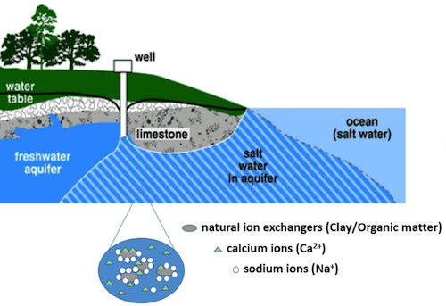
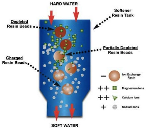
4.2 Reaction Thermodynamics and Important Parameters
Cation exchange reactions
Ion exchange reactions occur when ions exchange their positions at the soid-surface – water interface. These reactions are typically assumed reversible and occur instantaneously at time scales ranging from microseconds to hours. Ion exchange is typically represented in the following form:
Here (s) and (aq) refer to solid and aqueous phases, respectively; X- denotes the negatively charged surface sites that bound cations Au+ and Bv+, with u and v being the charges of A and B, respectively. In this reaction, A and B are cations that compete for sorption sites (Appelo and Postma, 1993; Sposito et al., 1981; Vanselow, 1932). The equilibrium constant Keq of reaction (1) can be expressed as
Here the parentheses [ ] represent activities. Aqueous concentrations are easily related to activities through concentration and activity coefficients. Activities of ions on solid phases are typically expressed as a fraction of the total, either as molar fraction or as equivalent fractions. The total number can be based on the number of exchange sites or as the number of exchangeable cations.
The units meq is often used in ion exchange calculations. An meq is the number of ions that sums a specific quantity of electrical charges. For example, an meq of K+ is about 6.02 x 10²⁰ positive charges. On the other hand, an meq of Ca2+ is also 6.02 x 10²⁰ positive charges, however only 3.01 x 10²⁰ ions because Ca2+ has two positive charges. For an ion Ii+ with a charge of i, the equivalent fraction bI is calculated as:
where I, J, K are exchangeable cation with charges i, j, k, respectively. A molar fraction $\beta_{I}^{M}$ is obtained by the following form:
Here TEC is the total exchangeable cations in mmol/kg sediment, not cation exchange capacity. The use of fractions should give the summation of fractions being 1, that is, .
Three common conventions used in writing ion exchange equilibrium constants are Gaines-Thomas convention, Gapon convention, and Vanselow convention. If the ion exchange is between cations of the same valence (homovalent exchange), the convention does not make a difference. If the exchange is between cations of different valences (heterovalent), the convention makes a difference. For example, the ion exchange reaction between Na and Ca can be written as follows:
With
Here if the equivalent fraction of the exchangeable cations is used for $β$ values, the Gaines-Thomas convention is followed (Graines and Thomas, 1953). If we use molar fractions for $β$ values, we follow the Vanselow convention (Vanselow, 1932). If the activities of cations on exchange sites are expressed as a fraction of the number of exchange sites (X-), we follow the Gapon convention, the reaction will be written as follows:
Where
Here the activities are expressed in terms of the mole fraction of the total number of exchangeable sites. To fully understand the difference between different conventions and calculation, please go over Example 6.3 in chapter 6 of Appelo and Postma (2005).
Selectivity coefficient
The capabilities of ions to compete for exchange sites are governed by their affinity to the surface of the exchangers. Selectivity coefficients have been reported in literature for common ions including Na+, K+, Ca2+, and Mg2+, however rarely for trace metals. The larger the selectivity coefficient, the higher affinity of the ion to the solid phase and the more competitive for exchange. In general, ions have high affinity to exchange sites when they have higher valence, are less solvated with water molecules, and react strongly with the surface sites. The following Table 1 lists selectivity coefficients reported in literatures for ion exchange on kaolinite (Appelo and Postma, 2005; Bundschuh and Zilberbrand, 2011).
| No. | Ion exchange reaction | log K |
|---|---|---|
| 1 | $2 \mathrm{Na}-X+\mathrm{Mg}^{2+} \Leftrightarrow \mathrm{Na}^{+}+\mathrm{Mg}-X_{2}$ | 0.60 (0.44 ~ 0.78) |
| 2 | $2 \mathrm{Na}-\mathrm{X}+\mathrm{Ca}^{2+} \Leftrightarrow \mathrm{Na}^{+}+\mathrm{Ca}-X_{2}$ | 0.80 (0.44 ~ 0.104) |
| 3 | $2 \mathrm{Na}-X+\mathrm{Ba}^{2+} \Leftrightarrow \mathrm{Na}^{+}+\mathrm{Ba}-X_{2}$ | 0.91 (0.44 ~ 0.104) |
| 4 | $2 \mathrm{Na}-X+\mathrm{Sr}^{2+} \Leftrightarrow \mathrm{Na}^{+}+\mathrm{Sr}-X_{2}$ | 0.91 (0.44 ~ 0.104) |
For typical ion exchangers, the sequence of affinity is as follows: Ba2+> Pb2+ > Sr2+ > Ca2+ > Ni2+ > Cd2+ > Cu2+ > Co2+> Zn2+ > Mg2+ > Ag+> Cs+ > K+ >NH4+ >Na+ >H+. When there are multiple cations co-exist in the solution, the surface exchange site composition is largely determined by the cation aqueous concentration and their affinity to the exchange sites. To calculate the exchange site composition, that is, the mole fraction of each cation on the exchange site, please follow the example 6.4 in chapter 6 of Appelo and Postma (2005).
Cation exchange capacity
The cation exchange capacity (CEC, meq/kg solid) is a measure of the solid phase capacity for ion exchange reactions (Meunier, 2005). The CEC of different porous media are very much associated with their clay content, organic carbon, and grain size. Different materials have different CEC values. CEC values of clay minerals such as muscovite, illite, kaolinite, and chlorite are high for their grain sizes smaller than 2 μm (Drever, 1982). In general, organic matter has the highest CEC values (1500 - 4000 meq/kg). Iron oxides play a vital role in natural processes and controls nutrient availability and heavy-metal mobility (Houben and Kaufhold, 2011). Iron oxides, such as goethite and hematite, have CEC values from 40 to 1000 meq/kg. Many solid materials have iron oxides or organic matters coated on their surface and therefore have large CEC values. For soils, CEC value is a function of solution pH depending on hydrolysis reactions of surface sites. In general, cation exchange occurs due to the broken bonds around the crystal edges, the substitutions within the lattice, and the hydrogen of exposed surface hydroxyls that may be exchanged. Higher pH values give rise to more negative charges on clay, resulting in higher CEC. CEC values increase as the grain size decreases due to the large surface area associated with smaller grains.
| Minerals | Grain size (μm) | Surface area (m2/g) | CEC (meq/kg) |
|---|---|---|---|
| Kaolinite | 0.1-5.0 | 5-20 | 30-150 |
| Illite | 0.1-2.0 | 15-40 | 150-400 |
| Montmorillonite | 0.01-1.0 | 600-800 | 800-1200 |
4.3 Setting up Ion exchange simulation in CrunchFlow
Example 4.1.
Marcellus Shale flow back and produced waters typically contains high concentrations of metals, including Na(I), Ca(II), Mg(II), Sr(II), and Ba(II) (Chapman et al., 2012). The release of Marcellus Shale waste water into natural soils and sediment can lead to ion exchange reactions and partition of surface sites between major cations. Here we set up a batch experiment in CrunchFlow to model the major cations exchange on clay surface from Marcellus shale produced water.
Assume that we have the following Marcellus water in a 300 ml batch reactor. The water is in equilibrium with partial pressure of CO2 at 3.15×10⁻⁴ atmosphere. Please note that the concentrations are in ppm and in mol/kgw. Both can be used directly in CrunchFlow.
| Component | Conc. (ppm) | Molar (mol/kgw) |
|---|---|---|
| pH | 7.02 | |
| Co2 (aq) | Co2(g), 3.15e-4 atm | |
| Na(I) | 7900.0 | 3.43e-1 |
| Ca(II) | 2774.0 | 6.94e-2 |
| K(I) | 82.5 | 2.11e-3 |
| Mg(II) | 239.0 | 9.83e-3 |
| Ba(II) | 183.0 | 1.34e-3 |
| Sr(II) | 6.5 | 7.38e-5 |
| C1(-I) | charge |
“Charge” means that the ion concentration is calculated from charge balance.
The water is in equilibrium with a sediment with kaolinite being the major clay with a specific surface area of 13.9 m2/g and a CEC value is 100.0 meq/kg (the units in CrunchFlow is eq/g). The kaolinite occupies 0.005 of the total volume.
The selectivity coefficient of the cations are as follows in the database (values from (Appelo and Postma, 1993; Li et al., 2010)):
| No. | Ion exchange reaction | log K |
|---|---|---|
| 1 | $\mathrm{Na}X\Leftrightarrow\mathrm{Na}^++X^-$ | 0.0 |
| 2 | $\mathrm{K} X \Leftrightarrow \mathrm{K}^{+}+X^{-}$ | -0.69 |
| 3 | $\mathrm{Ca} X_{2} \Leftrightarrow \mathrm{Ca}^{2+}+2 X^{-}$ | -0.39 |
| 4 | $\mathrm{Mg} X_{2} \Leftrightarrow \mathrm{Mg}^{2+}+2 X^{-}$ | -0.30 |
| 5 | $\mathrm{Ba} X_{2} \Leftrightarrow \mathrm{Ba}^{2+}+2 X^{-}$ | -0.45 |
| 6 | $\operatorname{Sr} X_{2} \Leftrightarrow \mathrm{Sr}^{2+}+2 X^{-}$ | -0.45 |
Questions
- Without having any aqueous complexation reactions for the cations, what are their concentrations in water and on the exchange site? i.e., mole fraction of each species on the exchange site. Compared to its own original total aqueous concentration, what is the mole fraction of each cation on its exchange sites? Please make a table and a figure comparing different species. Which one has the largest percentage of its own mass on exchange sites? Why?
- Rerun the simulation with the cations have some major aqueous speciation reactions that lead to the formation of the following aqueous complexes: Cl species (CaCl+, MgCl+, BaCl+, NaCl(aq), SrCl+), and OH- speices (CaOH+, MgOH+, BaOH+, NaOH(aq), SrOH+). Answer the same sets of questions as in question 1.
- Compare the answers in question 1 and 2, does aqueous speciation make a difference in ion exchange reactions? What is the major difference?
CrunchFlow setup summary:
To set up CrunchFlow simulation please read CrunchFlow manual page 62 – 63 for details. Please also refer to the Exercise 5: Cs exchange on Hanford sediments.
You will need to set up the ION_EXCHANGE key word block in the input file to define the name of the exchange site and give parameters related to ion exchange in the CONDITION block. In addition, you will also need to define exchange reactions and equilibrium constants in the “Begin Exchange” block. For example, if you call your exchange site “XKao”, then you have the following block:
ION_EXCHANGE
exchange XKao- on Kaolinite
convention Vanselow
END
The first line specifies name of the exchange site and the mineral that the exchange is on. The second line specify the calculation convention that is used.
Li Li: All right. Let's start the lesson on ion exchange. I discussed in the text that ion exchange is somewhat similar to surface complexation. But then you have multiple cations. And these cations have different affinity to the solid surface. So essentially, they are competing with each other. As one with high affinity and high concentration in the water phase, it ends up to have more on the solid phase.
So if you look at the Keq values of the different-- you can get more or less a sense of their relative affinity. But also, if one particular species has high concentration in the water, it also ends up to be more on the solid phase because it has high concentration if you write a Keq values. In order to get the Keq, you need higher corresponding solid phase concentration.
So let's look at the example. Actually, this really should be 4.1. And that's 3.1 So let's go through this example. And we'll talk about how to set it up. This example, I'm kind of thinking about Marcellus Shale water, produced water or flowback water. And you have some concentration. We know there are a lot of different cations in this type of water.
So I'm giving you a typical composition of Marcellus Shale water, with high sodium, chloride, calcium. But you also have barium, strontium. Actually, the barium, strontium concentration is relatively low in what you have here. So we are here.
And I'm giving you both PPM and mole per kilogram water. Actually both of them, you can put in directly. So it's your choice. Now, I'm saying you have 3,000 milliliter of batch reactives. And water is equivalent with partial pressure of CO2, which is this is atmospheric concentration of CO2, try to simulate condition in soil.
And then, I'm giving you this table that essentially can document the K value for each reaction process. And the question I'm asking you, the first is, without any aqueous complexation reaction. So you are not going to put-- you're still going to put OH minus, carbonate, and all that. But you are not going to put, for example, calcium chloride, calcium OH plus, and all these secondary species.
I'm asking you to see, how much is absorbed on the exchange site. And what is the percentage of the absorption on the exchange sites compared to its original total concentration. Essentially, I'm asking you to make a table for each major cation and list aqueous concentration column and list another exchange site column, and compare different species.
But also calculate the percentage of the ones that are on the exchange site. Because they all start with aqueous concentration. So comparing the absolute value sometimes does not tell a lot of things. So you need to normalize them to the original total concentration.
But then I also want you to look at, on the exchange site, how much is occupied by each of these cations? How much is sodium? How much calcium? How much is barium, strontium, et cetera. So that's the first question.
And then second question is, running the simulation with speciation or complexation reactions. List the formation of chloride species and OH minus species, all these listed here. And then I'm asking you to answer the same question. So comparing one to, essentially, you getting some information about how important are these aqueous complexation. Does aqueous complexation help or not help these cations to go on the service site?
So let's start doing this. We had a discussion today. And then you are saying, maybe you can start with a blank one. So today I'm going to start with a blank input file. Essentially, there's not much information there. Except that you will be doing like all the runtime parameters up there.
And I also put a bit of output keyword specification there. I put two spacial profile time points. So it will be running into 100 minutes. And then, initial condition, this is already specified. We will specify initial condition later.
So let's go through each agree grid block-- keyword block. First one is discretization. This one here, you essentially would specify the size. And we know it's one grid block. So you would be doing-- first of all, you need to put in the units for length.
And we talked about this is 300 milliliters. So if you want to put centimeters or meters, that's fine. Last time we put centimeters. So this time, maybe, we'll just put in meters to have some variation. So the distance unit will be meters. And then before, we always specify x zones. You essentially only have one species.
You will specify one zone. And then, because it's 300 milliliters, so that's 300 centimeters cubed. And converting to meters would be 3 times 10 to the minus 4 meters cubed. I mentioned before, this is essentially, when we do this, we specify that this is essentially the length of x zone.
But by default, you actually have y zone and z zone. And the code is going to assume in these other two directions that you don't specify, it's going to 1 meter and 1 meter. So here you have specified 0.003 meters. So essentially your volume is 0.0003 cubic meters, which is 300 milliliters.
So that's here. Now you specify, essentially, the size of your system. Now we probably can try this now, just to be sure that you are not making any mistakes taking this block. I always think it's a good practice to input one by one. And after each keyword block, you kind of check if everything is correct, you didn't make any wrong mistakes or whatever in the input file.
So the top one is read and write. But because we didn't specify any condition, it doesn't know what to do. That's OK. At least it didn't give me anything about like it's not specified correct or something like that. So let's do that again. Let's continue.
So let's specify primary species. And for that, we need to look at our table. So always put H plus first. I mentioned that before, probably multiple times. But it's worth to mention again. Always put H plus. And we know we have CO2 aq. So essentially, it follows that table. The system is with CO2 gas. So you need to put to CO2 aq. No, actually you don't need because it's just primary species.
And then you will be putting all the different species like sodium-- just calcium, potassium, magnesium, barium, strontium, and chloride. That's your primary species on the table.
But remember is that we also have kaolinite. And I mentioned that for each mineral you put-- so later on we'll put kaolinite in the mineral block. Remember that in order for it to work for the mineral you will need to look up what this mineral is made up of. So let's look through.
Let's open with Notepad. So let's search for kaolinite. Let's see what it can post up. So kaolin coming up. You have H plus, you already have. You have aluminum. You have silica, SiO2 aq H2O. So essentially it's aluminum silica. Because aluminum silicon is not there on the list, so let's put these two in so we don't get messed up.
So you would have aluminum. And then you have SiO2 aq. So these are the species we can think about it. So that's the primary species list.
Now I'm saying that we don't put any secondary species like the chloride OH species. But we still need to put OH- in. Because you can't do anything without OH-, because that's water dissociation-association. And then you also have CO2 species. So you have to have bicarbonate and carbonate species. So these are the main species that you have to complete.
So that's a secondary species. And gases, do we have gases? We do because we have the CO2 aq that is in equilibrium with gas. So you do need the CO2 gas phase. And then, you have ion exchange. So this is a new keyword block. We learned this in this unit.
So the key here is exchange, the keyword exchange. I shouldn't do it in Word. And then I'm going to give it a name, which is x representing surface species. But this one is on kaolinite. So let's do this. Let's call that. And this is on the mineral kaolinite. So essentially, you put as an exchange, you have the keyword block and name of the surface site, exchange site, and then the name of the mineral.
But also, the other thing you need to specify is what convention are you using for the calculation. We talked about three different-- like Vanselow, Gaines-Thomas for example. And let's here, let's do Vanselow. Vanselow is the one the most commonly used conventions. So that's ion exchange.
So this keyword block is somewhat new. And you need to think about, OK, doing that, your flux will be here. But again, here, you have the kaolinite. And you need to put in the mineral kaolinite there, the name there. If it's a mineral dissolution precipitation, you would need to put it in like kinetic information, for example, dissolution rates and everything. But here we are not really looking at it the dissolution precipitation kaolin. So we can just specify kaolinite.
So these are all the kind of building blocks of your system, chemistry building blocks of your system. And now we're going to specify what condition we have. And again, we're looking at the table we have. It's Table 3. So let's just copy the species from aqueous, the species we had before. And we'll copy it. And then we will add whatever concentrations they need to be.
We probably should have units first. Actually, in condition, we all need to specify units. And this will, let's say, do PPM. And we can do temperature. We must always do temperature, which is 25.0. You can specify H plus. But this table, I'm giving you 7.02. So it's easier to do just pH, which would be 7.02.
And you have CO2 aq, we discussed last time in last lesson, you can specify the CO2 concentration with gas phase in this way, when you have a specific at partial pressure of that gas. E minus 4, so that's for CO2. And then we have sodium, which is 7,900.0. Calcium, 2,774.0. And the you have potassium, 82.5.
I always think it's good to line up and make it neat and clean. Because if you're not clean and lined up and all that, it's very easy to make mistakes. It's almost like when you write code. You want to keep it very clean and organized so that minimizes the chance of making mistakes. And when you check, it's easier to see. So it's worth the effort. 6.5. And chloride, we'll be doing that with charge. So you just put the charge there.
How do I know that this is going to be positive charge without this? You can try database sweep first, if you want. But I kind of know because I know there's a lot of cations there. You see there's a lot of cations there. But there's almost the only species for now will be chloride in OH minus. And pH you know is 7. So OH would be 10 to the minus 7 or something. So it must be positive charged.
And then we don't really have much of the aluminum. But we can put, for example, let's say we did before with this small concentration, just 3%. It's there. Acidic. So these are the primary species, our total concentration of primary species.
Now I need to, so, in a beaker, that's the water phase composition. But then you also need to specify how much solids is there and how much surface area of a solid, how much CC and all of that. So let's say we have volume fraction of the kaolinite is 0.005. I think I didn't specify that in the file. Let's do that with sediment with kaolinite being the major-- with specific surface area. And then I'll add the kaolinite occupies 0.005 of the total volume.
So you can actually calculate that because you have 0.005. And then the total concentrated volume is 300 milliliters. So that means you have about 1.5 milliliter of the kaolinite. And we should specify the same thing in the input file. So leave a space line here just to have the division between the solid phase and aqueous phase.
So kaolinite, first thing you need to specify is 0.005 volume fraction. Actually, of the solid phase, all these-- So essentially, you have 0.005. So that's actually smaller. We started talking about it. We didn't really put the porosity. We actually should put a porosity there.
Let's finish this mineral for a specific surface area. We said it's 13.9 meters squared per-- so it's volume fraction first on solid phase, and then specific surface area using SSA in meters squared per gram.
So that's a mineral. But you also need to specify the surface site and exchange. So you have xkao, which is your name that's specified in the exchange. This needs to be consistent with the exchange grid block. And then you have this kaolinite CC, which specifies how much kaolinite exchange capacity you have.
Let's do a bit of calculation here. Let me just make some notes here. You have 100.0 meq per kilogram, which is essentially 100.0 eq per gram. And this is equivalent to 1.0 E minus 2 eq per 100 grams, and also equivalent to 1.0 E minus 4-- oh, I'm sorry. This is actually not right.
You have kilogram to gram. And then that's a solvent, And meq to eq is 10 to minus 3. So this is actually 1.0 E minus 4. This is essentially the same as-- let me check the units of CrunchFlow. It's eq per gram. So essentially, eq per kilogram.
So this will be actually-- we should convert to eq per kilogram. Already kilogram, so eq 100 times 10 to minus 3, which is 10 to minus 2. I'm sorry. This should be 10 to minus 1, essentially 0.1 eq per kilogram. We actually don't really need that. We can do our conversion.
Now, so that means you need to put-- because this is CrunchFlow units. So this will be essentially 0.1. So you specify the mineral volume fraction keq. But actually, OK, here I said we actually need a little bit porosity. So let's say you have-- we probably should say 99.5% is water. So you actually porosity of 9--
So actually I should put kaolinite being 100%, 1.0, meaning all the solid phase of the kaolinite, because this is saying the total volume. So the rest of it is all water. And then so your porosity is 0.995. And you have 100%. They're all on the solid phase. This is volume fraction on solid. You only have kaolinite. That's what I mean. So that's a condition.
So I guess, do we need anything else? We have the dimension. Let's just try that. Dimension, Vanselow, secondary species, primary species, and all that. So we should be OK. We don't need to do any timestamping. Let's try if it works.
So it'd be lesson 4.1.in. Specify porosity smaller than zero. Let's see. Must be somewhere, something wrong in the input file. Maybe it's error. I don't know. 0.0. Let's just try again. 4.1.in. Hm. Interesting.
A lot of times when it reports one error, a lot of times it's because something else is wrong. I wonder if this is it because I have it opened in the Word format. So let me just copy everything and open in Notepad and see if it's because of that.
And we're going to call it Lesson 4.1 again. And we specify lesson 4.1.in. OK, because I'm opening that. Let's see. Let's try it again.
I do have this just specified. OK, let's see. Hm. Because of this, I think it's still the original one. Now it's in the-- let's do this. Hm. That's very interesting.
Oh, the volume -- Let me just think about it. I might have forgotten in. It does need to be the volume fraction total. So then you can-- I just realized that.
So the original file was right. It is a total volume. It's not the solid phase. That kind of mistake was different type of information. So let's try it. I think that's a reason. Because I specified one here. And then, it was seeing porosity-- it specified that it was 1 kaolinite So it will say porosity is smaller than 1 or equal to zero essentially.
Let's try it again. I believe that is the error. Now it runs. OK, great. So you now see the process of doing this. I also make mistakes. And it takes time to debug and to realize what's wrong. And in this case, actually, what is wrong here, it is porosity. So it does point out to the right location. So the lesson here is volume fraction on total volume system.
So later on, if for example, if you have multiple minerals here, let's say you specify kaolinite, you specify calcite, another mineral. So volume fraction of the mineral and the volume function of the porosity needs to add up to be 1.0. That's what you need to remember. Or the a batch reactor.
So now we can look at the output file, essentially. Let's look at, well, two files here for each because I specified two different times. But you can imagine that they should be the same. I can tell because the ion exchange reaction occurs really fast.
It doesn't have time dimension. So it doesn't really matter if it's 100 minutes or it's 0.1 minutes. Because it reached equivalence instantaneously. So if you compare this exchange one versus exchange two, they should have the same concentration, essentially.
So you have one, two. It's the exact same. So this is the exchange output, essentially, specifying in mole per gram solid, how much sodium on the surface, how much potassium, how much calcium, magnesium, strontium.
And you can see from the list, the dominant species is sodium, and then followed by calcium. Both of these species are very high concentration in the solution. Let's look at the input file again. Let's look at the table again.
So sodium and calcium are the highest two concentrations. Potassium was relatively low. Magnesium, barium is in hundreds. And strontium has lowest concentration. So let's look at this again.
So more or less, in here, because of the huge difference in concentration, you end up the sodium has the higher concentration. Calcium has the second highest. And then you have magnesium, barium, and strontium. So magnesium is a bit higher than barium, too. So the last one is barium. So that's for the exchange site.
And then if you look at the aqueous site, let's look at total concentration. That'll give you how much is in the-- total concentration is not in log units. So you have pH. You have CO2. Sodium, sodium goes from-- actually it's-- now you think about it.
The output is all in mole per kilogram water. So it's actually probably better if you're using the input file mole per kilogram water. So you can look at the differences between the output, which is after the reaction, to before the reaction. So now you have sodium at 0.34. Potassium, this much.
And you actually can calculate, for example. So these are the concentrations. This is per kilogram water. So you know there's 300 milliliters water. So this concentration times the volume of the water, that gives you the mass in the water phase. And for the exchange site, it gives you in units of mole per kilogram per gram solid.
And you can assume that we know it's 0.005 of the total volume of kaolin. So we actually can calculate from the 300 milliliter times 0.005, which is 1.5 milliliter of kaolinite. And so it's 1.5 centimeters cubed of kaolinite. You can convert that to gram of kaolinite using the density of the kaolinite, give you the total gram of the solid phase. And that, you can convert to how much mass on the exchange site.
So with that calculation, you essentially will be able to calculate how much for each species is in water and how much is actually in the solid phase for each species, the percentage. So you know which one more, actually. So that's for aqueous phase and solid phase and all that.
So the second question for that is when you do include these aqueous complexations. Let's do that. I'm closing this, closing this. I'm going to add the secondary species, more species. So this, it would be having all the OH species and chloride species. So let's see. Let's go through the list.
You have sodium chloride, which is aq because it doesn't have charge. And then you could have NaOH aq. Let's just go through each species. And then there's sodium. You could have calcium chloride positive, calcium OH positive, then you have potassium chloride aq. And then CKOH aq, Mg, MgOH plus, BaCl plus, BaOH plus. What else? Strontium. OK. Strontium, Cl plus. Strontium OH plus.
When I input these, I always try to be very careful. And I probably mentioned that you cannot use tab in the input file. Also you cannot use comments on the middle of the line. When you need to comment, you need to start new line. Otherwise, it could get confused.
So I to be more careful when putting this input file. Because if you're not careful, you end up spending more time debugging and all of the frustration and all that. So keep things neat. And be careful when you input these. That will minimize the chance of making a mistake and that. I mentioned that before.
So then you can save that original output file to a different folder. Otherwise, because I run, it will override to the original file. Here, just for demonstration, I don't do that. So if I run it again, it will surely overwrite everything. That's fine.
Secondary species input file not find in database. Let's see what happens. Hm. We just run it and it works. So it must mean I either made some mistake or let's see. Secondary species input file not found in database. I'm pretty sure that's not true. I'm sure there is a database for CO3. I'm going to search for CO3.
It should be there. Because, otherwise the previous run wouldn't finish. So it's there. So there is nothing wrong with the database. So it must be the input file. It's almost always our fault, as you can tell. Secondary species, just make sure everything is-- hm.
Looks like there might be something wrong there because I couldn't go up. Oh, OK. So there's a lot of space there. And when it started lines, that space might be too long. So it couldn't-- OK. Let's just do it again. This is probably it, I think.
So when you do this, OK, so you have this. Try to not have too much space in between. Otherwise, the code cannot handle it if it's too long. There are certain character limits in each line that the code can process. Let's do it again. I think that's the problem.
4.1.-- Now it runs. So it runs and you can see from the date modified, it's just the right time. So that means it's all the output file updated. And if you look at the exchange again and compare to the previous one if you saved it-- so you will. When you do homework, you will need to save it and compare and see how much difference does it make.
We went through the output file. So I don't think I need to talk more. What you will need to do is in each CrunchFlow, the one without aqueous speciation, make a table for the mass fraction of each of aqueous phase and mass fraction of the solid phase on the exchange site. And then do that for each major cation.
And then, do the second question when you do have these aqueous complexation, how much difference does it make? And you can also check the specific concentration of all the aqueous species to see which one dominant and all that. And for this, if you want is all the dominant species, you don't need to open each exchange file and everything. You actually can just look at the output file, less than 4.1 output file. All the concentrations should be there.
I used the output file just for you to see what is in this output file. But in here, this part should have everything there. And this part might not give you the unit so you can actually dig into the exchange or exchange.out in this file to look if you forgot about units.
For solid, it's mole per gram. For aqueous, it's mole per kilogram water. So it'd have all the different species. It'd also have all the exchange concentration. It'd also have all the aqueous concentration there. So you have everything you need.
I'm going to stop here. And you saw me make mistakes and then we debugged it. Actually, both times the code pointed the right place that I made a mistake. The first one was porosity because I didn't put porosity right. I put high kaolinite 1.0, so there's no room for porosity.
The second one is CO3 minus minus, and there's too many blank space in front of that. So the code doesn't realize it. Anyway, so that's the two mistakes I made. Try to make it kind of no space, just do enter for each species. You'll be fine.
All right. So I'm going to stop here. And you'll be working on the homework and everything. Have fun.
Solution to Example 4.1
1) Without aqueous speciation reactions, the results are summarized in Table 5. Here we show a detailed calculation for Ca as an example.
CaXKao on exchange sites: The total cation concentration on the exchange sites (summation of all cations on exchange site) = $8.03 \times 10^{-5} \mathrm{mole} / \mathrm{g}$
The Ca fraction fraction $(\%)=1.54 \times 10^{-5} \mathrm{mol} / \mathrm{g} / 8.0 \underline{3} \times 10^{-5} \mathrm{mole} / \mathrm{g} \times 100 \%=19.3 \%$
Molar fraction (%) of CaXKao of original total Ca mass:
Batch reactor size: $0.3 \mathrm{L}=300 \mathrm{cm}^{3}$
Kaolinite volume: $300\mathrm{cm}^3\times0.5\%=1.5\mathrm{cm}^3$
Kaolinite molecular volume: $99.5 \mathrm{cm}^{3} / \mathrm{mole} $
Kaolinite molecular weight: 258 g/mole
So for the given batch reactor of 0.3 L, it has kaolinite volume of 1.5 cm3. Converting the kaolinite volume to the gram unit, $\left(1.5\mathrm{~cm}^3/99.5\mathrm{~cm}^3/\mathrm{mole}\right)\times258\mathrm{\ g}/\text{ mole }=3.89\mathrm{\ g}$
Number of mole of Ca on the exchange site: $1.54\times10^{-5}\mathrm{\ mol}/\mathrm{g}\times3.89\mathrm{\ g}=6.0\times10^{-5}\mathrm{\ mole}$
Number of mole of total Ca: $\text{ Ca: }6.92\times10^{-2}\mathrm{\ mol}/\mathrm{L}\times0.3\mathrm{\ L}=2.08\times10^{-2}\mathrm{\ mole}$
Ca fraction on the exchange site to total Ca: $6.0\times10^{-5}\mathrm{\ mole}/2.08\times10^{-2}\mathrm{\ mole}=0.289\%$
In Table 5, Na is the dominant cation on the exchange site (77.9%) because of its high concentration in water. Mg has the largest fraction (0.298%) of its own mass on the exchange site. The partition between mass in water and in solid phase depends on the intrinsic selectivity coefficient and original total aqueous concentration.
| Cation | *In water (mol/L) | On exchange site (mol/g solid) | Mole fraction (%) of total | Mole fraction (%) of its total mass) |
|---|---|---|---|---|
| Na+ | 3.44E-01 | 6.23E-05 | 77.9 | 0.235 |
| Mg2+ | 9.83E-03 | 2.26E-06 | 2.83 | 0.298 |
| Ca2+ | 6.92E-02 | 1.54E-05 | 19.3 | 0.289 |
| Sr2+ | 7.42E-05 | 1.62E-08 | 0.0202 | 0.282 |
| Ba2+ | 1.33E-03 | 2.90E-07 | 0.363 | 0.282 |
* Note that all the aqueous species are for total concentration, which means that we added up the concentrations of all relevant species. For example, for Ca2+, we added free Ca2+ and all other Ca-containing aqueous species including CaCl+ and CaOH+. 2) With aqueous speciation reactions, the results are summarized in Table 6. Ca has the largest percentage (0.296%) of its own mass on the exchange site, because Mg forms stronger aqueous complexes than Ca.
| Cation | In water (mol/L) | On exchange site (mol/g solid) | Mole fraction (%) of total | Mole fraction (%) of its total mass) |
|---|---|---|---|---|
| Na+ | 3.44E-01 | 6.18E-05 | 77.2 | 0.233 |
| Mg2+ | 9.83E-03 | 2.13E-06 | 2.67 | 0.281 |
| Ca2+ | 6.92E-02 | 1.58E-05 | 19.7 | 0.296 |
| Sr2+ | 7.42E-05 | 1.61E-08 | 0.0201 | 0.281 |
| Ba2+ | 1.33E-03 | 2.95E-07 | 0.369 | 0.287 |
3) Comparing Table 5 and 6, the speciation reactions do change cation concentrations on the exchange site and the molar fractions slightly. This is because the aqueous speciation affects the partition of cations between different species, thus determining the concentration of free available cation ions that are involved in ion exchange reactions. Aqueous speciation in question (2) leads to a different pattern of relative aqueous cation concentrations, which determines the cation concentrations on the exchange site. The speciation reactions in question (2) does not significantly change molar fractions. This is because in the current simulation set-up, the exchange sites are relatively limited compared to the aqueous cations. Thus, the molar fractions of cations on exchange sites to its original total concentration is small and relatively insensitive to the cation concentration changes on the exchange site. The situation would be different if the surface area, or CEC is much larger.
4.4 Homework Assignment
Question 1 (an extension of example 4.1):
As an extension of the example 4.1, we can look at different parameters and understand how they change the cation concentrations on the exchange site. Please include all Cl- and OH- aqueous complexes as in example 4.1. Please calculate the major cation concentrations on the exchange site (K, Na, Ca, Mg, Ba, Sr) by changing only the parameter discussed in each sub-question, with all other parameters being the same as those in example 4.1. For each sub questions, please plot major cation concentrations on the exchange site as the changing parameter.
- Specific surface area: 1.39, 13.9, and 139.0 m2/g;
- CEC: 10.0, 100, and 1,000 meq/kg;
- pH of the Marcellus water: 7.02, 8.00, 12.0. (Note that at pH=12.0, you need to use the Cl- concentration you got from pH = 8.0 and put Na+ as "charge" species)
For each question, calculate the mole fraction of each species on the exchange site, and the mole fraction of each species compared to its own original total mass. Please make a table and a figure comparing different species. Which one has the largest percentage of its own mass on exchange sites? Why?
Which parameter(s) have the largest impact on ion exchange reactions? In lesson 3 we learned that pH is important for surface complexation reactions. Does it make a difference for ion exchange reactions?
Question 2 (optional): This is part of problem 6.7 in chapter 6, A&P.
Read the paper (Valocchi et al., 1981). Native groundwater in the injection test of this paper had the composition of $Na^+=\ 86.5,\mathrm{\ Mg}^{2+}=18.2,\text{ and }\mathrm{Ca}^{2+}=11.1\mathrm{\ mmol}/\mathrm{L}$. Injected water has 14.66 meq Cl-/L. Selectivity coefficient were (Gaines and Thomas convention, activity = molal concentration) $\mathrm{K}_{\text{Na\Mg}}=0.54\text{ and }\mathrm{K}_{\text{Na\Ca}}=0.41$. Sediment $\mathrm{CEC}=750\mathrm{\ meq}/\mathrm{L}$ pore water. Calculate
- the composition of the exchange complex of native groundwater.
- the composition of water after the salinity jump, in equilibrium with the original exchange complex (compare with Figure 6.16).
- the composition of the exchange complex in equilibrium with injected water (cf. example 6.11
4.5 Summary
Ion exchange is an important chemical process in natural and engineered systems. Understanding ion exchange reaction is important for us to understand and predict the reactive transport and fate of chemicals in nature. Here we introduce the reaction thermodynamics of ion exchange, and the set up of ion exchange simulation in a well-mixed batch reactor in CrunchFlow.
References
(2008) St. Johns River Water Management District,. WaterWays: More about Water Below the Ground.
Appelo, C. and Willemsen, A. (1987) Geochemical calculations and observations on salt water intrusions, I. A combined geochemical/minxing cell model. Journal of Hydrology 94, 313-330.
Appelo, C.A.J. and Postma, D. (1993) Geochemistry, Groundwater and Pollution. A. A. BALKEMA PUBLISHERS
Appelo, C.A.J. and Postma, D. (2005) Geochemistry, groundwater and pollution. CRC Press.
Bundschuh, J. and Zilberbrand, M. (2011) Geochemical Modeling of Groundwater, Vadose and Geothermal Systems. CRC Press.
Chapman, E.C., Capo, R.C., Stewart, B.W., Kirby, C.S., Hammack, R.W., Schroeder, K.T. and Edenborn, H.M. (2012) Geochemical and Strontium Isotope Characterization of Produced Waters from Marcellus Shale Natural Gas Extraction. Environmental Science & Technology 46, 3545-3553.
Drever, J.I. (1982) The geochemistry of natural waters. Prentice-Hall, Englewood Cliffs, N.J.
G., C.J. (2008) Overexploitation and Contamination of Shared Groundwater Resources. Springer Netherlands.
Gregory, K.B., Vidic, R.D. and Dzombak, D.A. (2011) Water management challenges associated with the production of shale gas by hydraulic fracturing. Elements 7, 181-186.
Houben, G. and Kaufhold, S. (2011) Multi-method characterization of the ferrihydrite to goethite transformation. Clay Minerals 46, 387-395.
Kaushal, S.S., Groffman, P.M., Likens, G.E., Belt, K.T., Stack, W.P., Kelly, V.R., Band, L.E. and Fisher, G.T. (2005) Increased salinization of fresh water in the northeastern United States. P Natl Acad Sci USA 102, 13517-13520.
Li, L., Steefel, C.I., Kowalsky, M.B., Englert, A. and Hubbard, S.S. (2010) Effects of physical and geochemical heterogeneities on mineral transformation and biomass accumulation during biostimulation experiments at Rifle, Colorado. Journal of Contaminant Hydrology 112, 45-63.
Ma, C. and Eggleton, R.A. (1999) Cation exchange capacity of kaolinite. Clays and Clay Minerals 47, 174-180.
Marinsky, J.A. and Marcus, Y. (1995) Ion Exchange and Solvent Extraction: A Series of Advances. CRC Press.
Meunier, A. (2005) Clays. Springer, New York, Berlin.
Rodrigues, A.E. (1986) Ion exchange: science and technology. Springer.
Selim, H.M. (2012) Competitive Sorption and Transport of Heavy Metals in Soils and Geological Media. CRC Press.
Slomp, C.P. and Van Cappellen, P. (2004) Nutrient inputs to the coastal ocean through submarine groundwater discharge: controls and potential impact. Journal of Hydrology 295, 64-86.
Sposito, G., Holtzclaw, K.M., Johnston, C.T. and Levesquemadore, C.S. (1981) Thermodynamics of Sodium-Copper Exchange on Wyoming Bentonite at 298-Degrees-K. Soil Science Society of America Journal 45, 1079-1084.
Valocchi, A.J., Street, R.L. and Roberts, P.V. (1981) TRANSPORT OF ION-EXCHANGING SOLUTES IN GROUNDWATER - CHROMATOGRAPHIC THEORY AND FIELD SIMULATION. Water Resources Research 17, 1517-1527.
Vanselow, A.P. (1932) The utilization of the base exchange reaction for the determination of activity coefficients in mixed electrolytes. Journal of the American Chemical Society 54, 5.
Lesson 5: Microbe-mediated Redox Reactions
Overview
In this lesson we will learn about the thermodynamics and kinetics of microbe-mediated redox reactions, the biogeochemical redox ladder in natural systems, and setting up microbe-mediated reactions in well-mixed batch reactors.
Learning Outcomes
By the end of this lesson, you should be able to:
- Understand the general principles of microbe-mediated redox reactions, including microbial energetics and thermodynamics that determine the order of microbe-mediated reactions;
- Use microbial energetics to write reaction equations with microbial biomass as reaction products;
- Understand Monod rate laws and key parameters that control rates of microbe-mediated reactions;
- Set up simulations in CrunchFlow for microbe-mediated reactions in well-mixed reactors.
Learning Roadmap
| References (optional) |
|
|---|---|
| To Do |
|
Questions?
If you have any questions, please post them to our Questions? discussion forum (not e-mail), located in Canvas. The TA and I will check that discussion forum daily to respond. While you are there, feel free to post your own responses if you, too, are able to help out a classmate.
5.1 Importance of microbe-mediated reactions
Microorganisms are everywhere in the Earth surface environment. Their presence has significant influence in the natural and engineered environments. They play a key role in the biogeochemical cycling of elements such as carbon (C), oxygen (O) and nitrogen (N). For example, primary production involves photosynthetic microorganisms that transform CO2 in the atmosphere into organic (cellular) materials of vegetation in terrestrial systems. Planktonic algae and cyanobacteria on the other hand, are the “grass of the sea”. They account for ~ 50% of the primary production on the planet and are the primary carbon source for marine life. The fixation of N from the N2 gas also occurs through N-fixing microorganisms. Microorganisms are believed to be critical in the origin of life and in the transformation of rocks to soils that create life-accommodating environments on Earth. In the modern time when humans generated large quantities of waste and contaminants, microorganisms have overtaken the daunting tasks of cleaning up and recycling wastes in engineered systems such as wastewater treatment plants. They have also been indispensable in remediating contaminated water, soils, and aquifers.
5.2 Microbe-mediated reactions
For any redox reactions to occur, we need an electron donor and electron acceptor. The oxidation state of the electron donor increases during redox reactions, whereas that of the electron acceptor decreases. In natural environments, organic carbon often serves as the electron donor in microbe-mediated reactions and become oxidized from organic carbon to inorganic form (e.g., CO2), while multiple electron acceptors often co-exist, including oxygen, nitrate, manganese, iron oxides, among others. There are typically multiple functioning microbial groups that use different electron acceptors.
Biogeochemical redox ladder
Microorganisms typically do not use multiple electron acceptors simultaneously. Instead they use electron acceptors in the order of biogeochemical redox ladder, as shown in Figure 1 for some of the naturally-occurring electron acceptors. Different redox reactions release different amount of energy. For example, aerobic oxidation reactions generate much more energy than other redox reactions. The oxidation of glucose can produce 2,880 kJ / mol of C6H12O6; sulfate reduction can produce 492 kJ /mol of C6H12O6, as shown in Figure 2, a much smaller amount. The microorgnanisms that use high-energy-output redox reactions therefore has growth advantage and can outgrow other species.
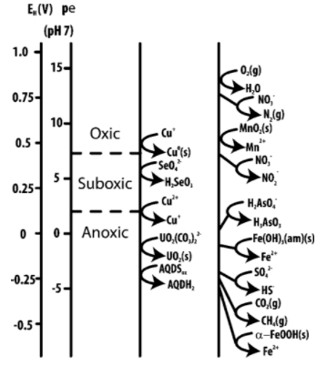
| Reactions | Chemical Formula | Free Energy kJ/mol glucose |
|---|---|---|
| Aerobic Oxidation | $\mathrm{C}_{6} \mathrm{H}_{12} \mathrm{O}_{6}+6 \mathrm{O}_{2} \rightarrow 6 \mathrm{CO}_{2}+6 \mathrm{H}_{2} \mathrm{O}$ | -2,880 |
| Denitrification | $5\ \mathrm{C}_6\mathrm{H}_{12}\mathrm{O}_6+24\mathrm{\ NO^-}_3+24\mathrm{\ H}^+\rightarrow\ 30\mathrm{\ CO}_2+42\mathrm{\ H}_2\mathrm{O}+12\mathrm{\ N}_2$ | - 2,720 |
| Sulfate reduction | $6\mathrm{\ C}_6\mathrm{H}_{12}\mathrm{O}_6\ +\ 6\mathrm{\ SO}_4^{2-}+9\mathrm{\ H}^+\rightarrow\ 12\mathrm{\ CO}_2+12\ \mathrm{H}_2\mathrm{O}+3\mathrm{H}_2\mathrm{S}+3\mathrm{HS}^-$ | - 492 |
| Methanogenesis | $\mathrm{C}_6\mathrm{H}_{12}\mathrm{O}_6\ \rightarrow\ 3\mathrm{\ C}\mathrm{O}_2+\ 3\mathrm{\ CH}_4$ | -428 |
| Ethanol Fermentation | $\mathrm{C}_6\mathrm{H}_{12}\mathrm{O}_6\ \rightarrow\ 2\mathrm{CO}_2\ +\ 2\mathrm{CH}_3\mathrm{CH}_2\mathrm{OH}$ | -244 |
*Table modified from Rittman and McCarthy, 2001. Used with Permission
Writing microbe-mediated reactions
Redox reactions written in the form shown in Figure 2, do not consider microorganisms or biomass as part of the reaction products. In order to do so, we need to consider reaction energetics and metabolic pathways. The catabolic pathway breaks down the electron donor (e.g., organic carbon) into smaller molecules and generates energy. The anabolic pathway uses organic carbon and energy harnessed in the catabolic pathway to synthesize large cell molecules. The two pathways complement each other in that the energy released from one is used up by the other. The degradative process of a catabolic pathway provides the energy required to conduct a biosynthesis of an anabolic pathway. Both pathways use electrons from the electron donor. Therefore, electrons from the electron donor partition into the two pathways. To write the full reaction equations, we will need to know the fractions of electrons being used for energy production (fe) and for cell synthesis (fs). The summation of $\ f_e\ and\ f_s\ is\ 1.0$. For different redox reactions, these fractions differ. Those higher in the biogeochemical redox latter generate more energy per electron flow so they need smaller fractions of electrons for energy production (smaller fe) and can channel more electron into cell synthesis. Therefore, values of fe increase and fs decrease as we go from aerobic oxidation that is high in the redox ladder to those lower in the redox ladder. That is, less microbial cells are being produced as we go down the redox ladder with the same amount of electron donor. To write the full reaction equation, we also need chemical formula for microbial cells. A commonly used one is C5H7O2N, approximating the ratios of major elements C, N, O, H, in biomass without including trace elements such as phosphorous, sulfur, metals, etc. Other examples include C8H13O3N2, often used to represent microbial sludge produced in waste water treatment plants. Details of how to write such reaction equations are given in Chapter 2 of Rittmann and McCarthy (2001). Here we show a few examples of reaction equations with biomass as the product using acetate as the electron donor (Cheng et al., 2016; Li et al., 2010). Note that for the text below, the overall reactions R is developed using half reactions of electron donor (Rd), electron acceptor (Ra) and cell synthesis (Rc). The energy production reaction Re = Ra - Rd and cell synthesis reaction Rs = Rc - Rd, respectively. The overall reaction $\ R\ =\ f_e\ R_e+f_s\ R_s=\ f_e\ \left(R_a-R_d\right)+f_s\ \left(R_c-R_d\right)=f_e\ R_a+f_s\ R_c-R_d$. A few examples are shown below.
Aerobic oxidation:
$R_a\ \left(Reaction\ of\ electron\ acceptor\right):\frac{1}{4}O_2+H^++e^-=\frac{1}{2}H_2O$
$\mathrm{R_d\ \left(Reaction\ of\ electron\ donor\right)}:\ \frac{1}{4}\mathrm{HCO}_3^-+\frac{9}{8}\mathrm{H}^++e^-=\frac{1}{8}\mathrm{CH}_3\mathrm{COO}^-+\frac{1}{2}\mathrm{H}_2\mathrm{O}$
$R_c\ \left(Cell\ synthesis\ reaction\right):\ \frac{1}{4}HCO_3^-+\frac{1}{20}NH_4^++\frac{6}{5}H^++e^-=\frac{1}{20}C_5H_7O_2N_{AOB}+\frac{13}{20}H_2O$
Here AOB represent aerobic oxidating bacteria.
The catabolic pathway Re = -Ra - Rd that yields: $\frac{1}{8}CH_3COO^-+\frac{1}{4}O_2=\frac{1}{4}HCO_3^-+\frac{1}{8}H^+$
The anabolic pathway RS = Rc - Rd that yields:
$\frac{1}{8}CH_3COO^-+\frac{1}{20}NH_4^++\frac{3}{40}H^+=\frac{1}{20}C_5H_7O_2N_{AOB}+\frac{1}{20}H_2O$
Combining the two pathways using $R\ =f_e\cdot\left(R_a-R_d\right)+f_s\cdot\left(R_c-R_d\right)=f_e\cdot R_a+f_s\cdot R_c-R_d,$
with $\ f_e=0.4\ and\ f_s=0.6$, we have the following:
$\begin{array}{l}R:0.100\mathrm{O}_2(aq)+0.125\mathrm{CH}_3\mathrm{COO}^-+0.030\mathrm{NH}_4^+\rightarrow\\
0.030\mathrm{C}_5\mathrm{H}_7\mathrm{O}_2\mathrm{~N}_{\mathrm{AOB}}+0.100\mathrm{HCO}_3^-\ +0.090\mathrm{H}_2\mathrm{O}+0.005\mathrm{H}^+\end{array}$
Denitrification
$R a: \frac{1}{5} N O_{3}^{-}+\frac{6}{5} H^{+}+e^{-}=\frac{1}{10} N_{2}+\frac{3}{5} H_{2} O$
$\mathrm{Rd}: \frac{1}{4} \mathrm{HCO}_{3}^{-}+\frac{9}{8} \mathrm{H}^{+}+e^{-}=\frac{1}{8} \mathrm{CH}_{3} \mathrm{COO}^{-}+\frac{1}{2} \mathrm{H}_{2} \mathrm{O}$
$R c: \frac{1}{4} H C O_{3}^{-}+\frac{1}{20} N H_{4}^{+}+\frac{6}{5} H^{+}+e^{-}=\frac{1}{20} C_{5} H_{7} O_{2} N_{N R B}+\frac{13}{20} H_{2} O$
$\text{ Following }R=f_e\cdot R_a+f_s\cdot R_c-R_d,\text{ using a higher }f_e=0.45,\ f_s=0.55,$ we have:
$\begin{array}{l}R:\ 0.090\mathrm{NO}_3^-+0.125\mathrm{CH}_3\mathrm{COO}^-+0.0275\mathrm{NH}_4^++0.075\mathrm{H}^+\rightarrow\\
0.0275\mathrm{C}_5\mathrm{H}_7\mathrm{O}_2\mathrm{N}_{NRB}+0.1125\mathrm{HCO}_3^-+0.1275\mathrm{H}_2\mathrm{O}+0.015\mathrm{N}_2(aq)\end{array}$
Iron reduction reaction
$\mathrm{Ra}:\mathrm{\ FeOOH}(s)+3\mathrm{H}^++e^-=\mathrm{Fe}2^+2\mathrm{H}_2\mathrm{O}$
$\mathrm{Rd}:\ \frac{1}{4}\mathrm{HCO}_3^-+\frac{9}{8}\mathrm{H}^++e^-=\frac{1}{8}\mathrm{CH}_3\mathrm{COO}^-+\frac{1}{2}\mathrm{H}_2\mathrm{O}$
$Rc:\frac{\ 1}{4}HCO_3^-+\frac{1}{20}NH_4^++\frac{6}{5}H^++e^-=\frac{1}{20}C_5H_7O_2N_{\mathrm{Fe}RB}+\frac{13}{20}H_2O$
$\text { Following } R=f_{e} \cdot R_{a}+f_{s} \cdot R_{c}-R_{d}, \text { where } f_{e}=0.60, f_{s}=0.40$
$\begin{array}{l}\mathrm{R}:\mathrm{\ FeOOH}(\mathrm{s})+0.208\mathrm{CH}_3\mathrm{COO}^-+0.033\mathrm{NH}_4^++1.925\mathrm{H}^+\rightarrow\\
\mathrm{R}:\mathrm{\ FeOOH}(\mathrm{s})+0.208\mathrm{CH}_3\mathrm{COO}^-+0.033\mathrm{NH}_4^++1.925\mathrm{H}^+\end{array}$
Sulfate Reduction
$\mathrm{Ra}:\ \frac{1}{8}\mathrm{SO}_4^{2-}+\frac{9}{8}\mathrm{H}^++e^-=\frac{1}{8}\mathrm{HS}^-+\frac{1}{2}\mathrm{H}_2\mathrm{O}$
$\mathrm{Rd}:\ \frac{1}{4}\mathrm{HCO}_3^-+\frac{9}{8}\mathrm{H}^++e^-=\frac{1}{8}\mathrm{CH}_3\mathrm{COO}^-+\frac{1}{2}\mathrm{H}_2\mathrm{O}$
$Rc:\ \frac{1}{4}HCO_3^-+\frac{1}{20}NH_4^++\frac{6}{5}H^++e^-=\frac{1}{20}C_5H_7O_2N_{\mathrm{Fe}RB}+\frac{13}{20}H_2O$
$\text{ Following }R=f_e\cdot R_a+f_s\cdot R_c-R_d,\text{ where }f_e=0.92,\ \ f_s=0.08,$
$\begin{array}{l}R:\ 0.125\mathrm{SO}_4^{2-}+0.13525\mathrm{CH}_3\mathrm{COO}^-+0.004375\mathrm{NH}_4^++0.0065\mathrm{H}^+\rightarrow\\
R:\ 0.125\mathrm{SO}_4^{2-}+0.13525\mathrm{CH}_3\mathrm{COO}^-+0.004375\mathrm{NH}_4^++0.0065\mathrm{H}^+\end{array}$
In each of these reactions, the ratio of the biomass carbon number (C) in the biomass formula (C5H7O2N) produced per C of organic C is called yield coefficient. For example, for aerobic oxidation, the yield coefficient is 0.030*5/(0.125*2) = 0.60; for denitrification, the yield coefficient is 0.0275*5/(0.125*2) = 0.55; for the FeOOH reduction reaction, the yield coefficient is 0.033*5/(2*0.208) = 0.40; for the sulfate reduction reaction, the yield coefficient is 0.004375*5/(2*0.13525) = 0.08 C biomass /C organic. In general, large fs values leads to high yield coefficients. Values of fs are typically in the range of 0.6 – 0.75 for aerobic oxidation, 0.55 – 0.7 for denitrification, and 0.08 – 0.30 for sulfate reduction. For typical values of different types of redox reactions, please refer to Rittmann and McCarthy (2001).
5.3 Monod Rate Laws
Dual Monod kinetics
The kinetics of microbe-mediated reactions are often described by Monod rate laws in the following form:
Here $\mu$ is the rate constant (mol/s/microbe cell), $C_{C_{5} H_{7} O_{2} N}$ is the concentration of microbe cells (cells/m3), Cd and Ca are the concentrations of electron donor and acceptor of the reaction (mol/m3). The Km,D and Km,A are the half-saturation coefficients of the electron donor and acceptors (mol/m3), respectively. These coefficients are the concentrations at which half of the maximum rates are reached for the electron donor and acceptor, respectively. If the electron donor is not limiting, it means that $C_{D} ? K_{m, D}$, so that the term $\frac{C_{D}}{K_{m, D}+C_{D}}$ is essentially 1.
Dual Monod kinetics with inhibition term
In order to represent the biogeochemical redox ladder, we will need to introduce an additional term in the dual Monod rate law, the inhibition term. A Monod rate law with an inhibition term looks as follows:
Here the KI,H is the inhibition coefficient for the inhibiting chemical H. In contrast to the Monod terms, the inhibition terms become 1 (not inhibiting) only when KI,H?CH.
As an example, in a system where oxygen and nitrate coexist, which is very common in agricultural soils, aerobic oxidation will occur first before denitrification occurs. The sequence of that can be represented by the following:
These two rate laws, with proper parameterization, will ensure that denitrification reaction occurs only when O2 is depleted to a certain extent that the term $\frac{K_{I, O_{2}}}{K_{I, O_{2}}+C_{O_{2}}}$ approaches 1.0. If other electron acceptors that are lower than nitrate in the redox ladder also occur, then multiple inhibition terms are needed. For example, if there is also iron oxide in the system, we will need the following for the iron reduction rate law:
Where the additional litrate inhibition term will allow iron reduction to occur at sufficiently significant rates only when nitrate level is low compared to the inhibition constant value.
5.4 Setting up in CrunchFlow Example 5.1
The system: I have a 200 ml bottle in my kitchen. I accidentally drop some recently-fertilized soil grains from my backyard into the bottle. I close the bottle after the accident. The soil has some microbial cells, along with some organic carbon (assuming the formula of acetate), and nitrate. The initial acetate and NO3 concentration in the bottle are 5.0 and 1.0 mmol/L, respectively. Assume initially there are some dissolved O2 in the water at the concentration of 0.28 mmol/L while all other chemicals in the soil are not reactive. The initial biomass concentration of O2-reducing and nitrate-reducing biomass are 2.0×10⁻⁶ and 1.5×10⁻⁶ mol-biomass/L, respectively. In the bottle, I put in some magic powders (to be invented in the future by my daughter Melinda Wu!) that would automatically show the concentrations of chemical species without the need of measurements (that would be my dream come true!). The microbe-mediated reactions advance as the follows:
Aerobic oxidation $\left(f_{s}=0.6 \text { and } f_{e}=0.4\right)$:
$\begin{array}{l} 0.500 \mathrm{O}_{2(a q)}+0.417 \mathrm{CH}_{3} \mathrm{COO}^{-}+0.067 \mathrm{NH}_{4}^{+} \rightarrow \\ 0.067 \mathrm{C}_{5} \mathrm{H}_{7} \mathrm{O}_{2} \mathrm{~N}_{\mathrm{AOB}}+0.500 \mathrm{HCO}_{3}^{-}+0.200 \mathrm{H}_{2} \mathrm{O}+0.150 \mathrm{H}^{+} \end{array}$
Denitrification $\left(f_{s}=0.55 \text { and } f_{e}=0.45\right)$:
$\begin{array}{l} 0.090 \mathrm{NO}_{3}^{-}+0.125 \mathrm{CH}_{3} \mathrm{COO}^{-}+0.0275 \mathrm{NH}_{4}^{+}+0.075 \mathrm{H}^{+} \rightarrow \\ 0.0275 \mathrm{C}_{5} \mathrm{H}_{7} \mathrm{O}_{2} \mathrm{~N}_{\mathrm{NRB}}+0.1125 \mathrm{HCO}_{3}^{-}+0.1275 \mathrm{H}_{2} \mathrm{O}+0.045 \mathrm{~N}_{2(a q)} \end{array}$
| Reactions | $\mu_{\max }(\text { mol/mol-biomass/yr) }$ | $\begin{array}{c} K_{m, \text { acceptor }} \\ \text { (mol/kgw) } \end{array}$ | $\begin{array}{c} K_{m, \text { donor }} \\ \text { (mol/kgw) } \end{array}$ | $\begin{array}{r} K_{I, O 2(a q)} \\ (\mathrm{mol} / \mathrm{kg} \mathrm{w}) \end{array}$ |
|---|---|---|---|---|
| Aerobic | 50000 | 1.00x10⁻⁴ | 1.00x10⁻³ | |
| Denitrification | 20000 | 1.00x10⁻³ | 1.00x10⁻³ | 1.00x10⁻⁶ |
*Range of relevant parameters is from Cheng et al., 2016; Li et al., 2010.
Questions:
- Which reaction would occur first?
- What do you expect to see the evolution of the concentrations for the species: acetate, O2(aq), nitrate, total inorganic carbon, and biomass for denitrifiers. Plot their concentrations as a function of time in the same figure.
Please watch the following video: Microbe Mediated Reactions (24:50)
Click for a transcript of the Microbe Mediated Reactions video
Microbe Mediated Reactions
Li Li: So let's get started. This is lesson 5, so we'll be talking about microbe-mediated reactions. I put in the reading materials the importance of microbe-mediated reactions-- how ubiquitous they are in natural environment. And we also talked about the biogeochemical redox ladder in the reading material. So things happen in sequence.
And then we have this example of-- we're talking about soils, so I grabbed some soil in the back yard, putting it in a water bottle in the kitchen. So this is the cup, I would say. So that's the system we have. In that example, we put some soil there. Let's close it. We have some water there. So we have some soil. Let's just put these as grains.
And the water originally has some oxygen in it. And I told you that the soil that I have we just recently fertilized. That means you will have nitrate in the system. So essentially, in the system, you have oxygen and nitrate as electron acceptors. And typically, for example, the soil usually have bacteria already there. Microbes is everywhere. They do a lot of work.
And also, usually, you would expect the soil carbon have-- the soil have some organic material. So essentially, it also have organic carbon, which we use acetate to represent that. So essentially, we're talking about a system that has water in it. It's well mixed. It has bacteria in it. So let's use that to represent bacteria. And it has two electron receptors, oxygen and nitrate. Perfect.
We have a system. We know it's going to have something going on, right? And again, this is well mixed. We are not talking about the advective transport, dispersion-diffusion yet. So this is a well-mixed system, meaning there's no concentration gradient in the system.
Now, then, the other system you have-- so you have microbes We use microbes The formula for bacteria is C5 H7 ON. Something like that. And it depends on what type of bacteria it is. If it's using oxygen, then we put oxygen on the side, just to indicate this is oxygen-reducing bacteria. If it's nitrate-reducing bacteria, we put nitrate there, just to distinguish between the two different bacteria. So essentially, you have two types of bacteria there in the system.
That's the system you have. And what's there? All the players, right? Now, we think about the reactions, what are the reactions? So first of all, we talk about, in the biogeochemical redox ladder, oxygen is the one that is going to be used first, because usually it has fast reaction rate. The microbes also get more energy out of it. So that means it has growth advantage, because it can grow more with the same amount of organic carbon they have. So the first one we call aerobic oxidation, meaning you have the transformation from CH3-- we use acetate to represent organic carbon. I'm not putting all these numbers into stoichiometrics. But essentially, just writing what are the major products.
So organic carbon will become oxidized to become bicarbonate or other forms of carbon. If it's relatively acidic condition, you might have CO2 gas coming out. And you have water or hydrogen under whatever condition it allows. And then you would grow bacteria.
So bacteria is also one of the products that we talk about. It'll has N. And then producing the oxygen. It's oxygen-reducing or aerobic bacteria or microbes. So that's the oxygen related reaction.
So we talk about, OK, that reaction will happen first. And remember, this is a closed system, meaning we have a certain amount of oxygen dissolved at first, and then it's going to be depleted over time because of reaction. So the microbes will be using this up. And then, the next steps, the next reaction that's going to happen will be denitrification.
So You will have, again-- that's assuming we will have plenty of organic carbon there. So then you will have nitrate. Again, there will be inorganic carbon become produced. It's the same process, If you think about it, as the human system. We breathe oxygen. We eat food, like grains, bread, rice, different type of, essentially, organic carbon. And then we breathe out CO2, which essentially is another form of bicarbonate, right? And then the water. Let's not write that.
And then you have another type of bacteria coming-- microbe coming out, which will be the denitrification microbe. So these are the two drivers of the system. But then, typically, you would also have-- I'm just writing at the side-- there should be a somewhat fast reaction compared to these microbe-mediated reaction. Would be the transition between CO2 aq, bicarbonate, and carbon. These are the inorganic carbon species that we know is going to happen. We talk about that in aqueous speciation or aqueous complexation reactions that we discussed before. So these are very fast reactions. So the major drivers are really these. And if we have other species, for example, calcium or magnesium, if there's plenty of them, there might be precipitation come, because these reactions will produce a lot of bicarbonate. And bicarbonate can-- when the condition allows, it could precipitate calcite, for example.
We're not going to focus on these. Our major goal right here, right now, is talking about these drivers. And if there's applications that you will need to consider these as something that would be specific about particular applications.
So we have these reactions. These are the processes we focus on. And then we'll be thinking about the species. What other species are there? So, for sure, we would have all the electron acceptors there, which is oxygen-- it dissolved oxygen. You have nitrate. You have its CH3 COO. These are the variables that we are solving for in these equations.
And then we also have-- let's put bicarbonate. But we know this is going to be also carbonate, CO2 aq, or H2 CO3. These three are almost like equivalent with each other. Hydrogen ion, for sure, and then it goes with OH-. Electron acceptor, electron donor, products. Nitrogen is-- did I write? OK. Here, I should add another, which is the product of denitrification. One product of denitrification will be N2. There could be a lot of-- a few other intermediate reaction products, like NO2-. People have seen that. Or ammonia, even. This could happen too. We're just using this as an example. So N2. So these are the major species.
But also, when we solve for these, when we are writing these four reactions in terms of these reactions. Microbe as products. We also should have C5 H7 ON0 O2. And then C5. These are the two major products too. It's not just the abiotic species. We would consider the microbes are the products of this reaction too. So these are the species that you are solving.
So we are not talking about other complexation reactions. So really, we're focusing on these species. And you probably quickly know, by this time, these are the-- these could be the second species, second species, second species. These are the things that we consider. And then the primary species would be oxygen, nitrate, this, this, hydrogen, N2, N2, and this. These are the primary species. Let me just write as primary to indicate the color. So that's what you have in terms of variables that we are solving for. Now, again, we are talking about the well-mixed system. So when we think about the reactions, the equations, it would be really the reaction in terms-- for example, for oxygen, you have something like this. It would be dc dt for oxygen, for example.
Oxygen is being consumed. So the volume-- so it's really volume of the bottle, the mass, and then times this dc dt. But then you also have, essentially, the mu. The mu-- let's call this mu as the stoichiometric coefficient. Fish It's consuming. It's in the left-hand side of the reaction, meaning it's being consumed. So this is stoichiometric. If, for example, this is 0.5, this value will be 0.5. And then we will be-- we think about the consumption. The rate of this will follow Monod, dual Monod kinetics. So you would have this mu max for oxygen term. And then we have this-- how much bacteria there. So it'll be the C5 H7 O2 N.
I should have an O2 here. That's why I feel something is missing. It's weird. O2. It should all have O2 there. All right. So you have these species, O2, and this is oxygen-reducing bacteria. So $\mu$ max, concentration of biomass, and then you should have two Monod terms. One is for concentration of oxygen, and then the Km oxygen plus concentration of O2. That's an electron acceptor. And then you have the C-- . Sorry, I am writing a bit of-- so this would time, right? So Km, and then the plus C acetate. CH3. I can't write anymore, but you know what I mean. So this is electron. Donor term electron. Acceptor term biomass. Maximum reaction rates. So that's for oxygen.
Similarly, you would write this for V dc. It's also being consumed. So essentially you would have the same, but you will have mu of CH3 COO- and the same expression. Right? It's the same reaction. We just consume different chemical species in different proportions. And you would write again, also, for bicarbonate. That's one of the products. So you really should have positive sign before this. So you have to write V dc dt. This would be like total carbon. And then $\mu$ of bicarbonate. So all this goes on. So you will be writing for all these.
Now, when you are write for-- so if you only have oxygen, you would have oxygen, this acetate, bicarbonate, and other species. That's good enough. But if you have nitrogen, then your equation for nitrogen would be a little bit different, in the sense that you would have the would same. But they would be replaced by nitrate acetate. But you will have the inhibition term by oxygen, because oxygen would act as inhibitor for denitrification to occur. When you have plenty of oxygen in the system, denitrification is not going to happen. Only after this concentration of oxygen has been decreased to levels that this term is more or less much higher than this, then this value would be close to 1. Then denitrification really kicks in. So that's for nitrate. Also notice, when you have both electron acceptors, this reaction will be happening at the same time just, at first, oxygen what will be the dominant one, because this term will have very small value, will inhibit denitrification to happen. But then this, the rate of this will become smaller and smaller because oxygen becomes smaller concentrations, this term becomes bigger and bigger. So there's a switch between different electron acceptors. The other thing is when you have multiple electron acceptors, when you write these acetate equations or when you write these for the produced inorganic carbon, you need multiple terms too, because the denitrification process also contributes to the consumption of acetate and production of bicarbonate. These are common products or common reactants. So you have multiple terms if you have the nitrate-related term.
I'm not going to detail everything. But essentially, that's what you think would have. So solving these equations. Let's say you have all the species. You'll be writing how many independent equations for primary species. And you have three fast reactions that you can form algebraic relationship to solve these other secondary species. You solve everything as a function of time. So this is dt. This is not partial t. Now, in that case, what do you think will happen when we have these products? So I talk about we have some magic powder putting in the bottle will help us. We read our numbers. What do you think will be the trend of, for example, oxygen? And what's going to be the trend of temporal evolution of nitrate. Using nitrate for this one. How do you think they are going to look like in terms of curve? So that will be actually the output of the model. You can see about how it was going to happen. So aerobic oxidation going to happen. First, oxygen concentration is going to be consumed first, then decreased. So let's say it's maybe oxygen starts from here. You see a decreasing trend of oxygen. Let's say it's something like that.
And then, what about nitrate? So nitrate is-- at first, because it was in the presence of oxygen, you wouldn't see much of nitrate decreasing. So it probably, at the beginning, it's going to, let's say, start from somewhere here. It'll be relatively flat. But it also, when the nitrogen-- I'm sorry. When the oxygen starts to decrease, it just start to show a sign of-- it depends on rates. How fast, how long it'll take. It depends. So when it's like almost completely depleted, then you would have nitrate kind of going full swing. And then it's going to decrease really fast. But then, when you think about the products, this produced N2. So N2, let's say, at the beginning, it's not much. It's almost zero. Now, when nitrate starts to be denitrified, then N2 starts to increase. Increase. It's almost like in the mid-- it almost mirrors nitrate. So this would be N2. That's the product of denitrification. Oxygen decrease, followed by nitrate decrease, and oxygen increasing.
What if you also have sulfate? Let's use another color. Let's use blue again. What if you have nitrate? So let's assume there's no ion there. So when you have sulfate-- so there's another electron acceptor, which is sulfate, which is also pretty active in subsurface environment. Probably not in very shallow soil, but in bit of deeper, when you don't have a lot of oxygen, you tend to have sulfate.
So sulfate would be probably, let's say, something like-- let's start here. It would start to become decreased when this denitrification happen. Then the concentration decreases. Then it will also follow maybe one-- depends on how much electron donors you have and acceptors. This is representing sulfate. And the product of that is sulfides. So sulfides probably would be small at the beginning. But then it'd be increasing over time. Something like that. Call it HS-. This is like randomly ending. Another electron, except it's not easy equation. But if you need to write for sulfate too, then you would have three major microbe-mediated reactions. And in addition to that, you would also have an equation related to sulfate and sulfide production. And notice, also, sulfate reduction will be inhibited by both oxygen and nitrates. So you have two inhibition terms. So in that case, only when oxygen and nitrate is depleted to pretty small amount, then the sulfate reduction can start occurring. So these inhibition terms really would ensure the biogeochemical redox ladder in the system.
OK. So that's what we have for this unit, for this lesson. And you can use this. Will set up stage for you to do the homework. Think about different reactions that are going to happen in sequence in natural systems-- in soil, aquifers, and then how microbes evolve and the different concentrations involved with time.
Actually, we didn't talk much about microbes. But the microbial concentration will increase over time, following where the-- different types will be following their own electron acceptor. Electron acceptor evolution. Oxygen decrease and aerobic microbial will be increased. Things like that. OK. So let me stop here, and you are ready to do the homework. Thank you.
How to simulate microbe-mediated reactions in CruchFlow (based on the simulations in previous lessons):
Please watch the following video (29:51):
Li Li: OK. Let's look at this example 5.1, which we are going to set up control rounds for microbe-mediated reaction. So system is still a closed system with a bottle, which means we don't have flow comes in, flow comes out. We're really focused on the reaction itself.
And you imagine there's a bottle, 200 milliliter in volume. We have soil which contains some organic carbon. We also have nitrate and oxygen in the system.
And then we also have these magic powder, et cetera, which we're very excited about. Everything is ready to do this. Now, these two reactions that I put here, aerobic oxidation, denitrification reaction, these two reaction is already written as an outcome of a half reactions that we discussed earlier with these specified energy petitioning proficient in term how much goes into catabolic pathways, how much goes into the anabolic pathways. OK. So here we are looking at these two interaction, imagining that these are happening. Aerobic oxidation should occur first before denitrification. I also put the rate of kinetic parameters here.
So we have $\mu$ max, Km, which are half saturation constants, and inhibition coefficient, which is Ki for denitrification reaction because it's going to be inhibited by the presence of oxygen. OK. And then we are charged to answer the question, which reaction would occur first, which I already told you. But we are going to look at what is the magic powder, of course. We are going to look at just the evolution of the concentrations for different species. How does acetate concentration, which is organic carbon, evolve over time? In addition, we are looking at oxygen nitrate, totally organic carbon, biomass, et cetera.
So let's look at our folder. Now here when you look at this there are several reactions. I'm sorry. There are several files. The same one is the Input file. There's one Database file, which is Old Rifle Database. That one is a regular database that you have seen before similar to like the database datcom .dbs, which has a lot of fraction equivalent constants, reaction stoichiometry, and primary species, second species, and all that. That's the same.
One major thing that is different is now here you have two more database file, which is AqueousMicrobe and SolidMicrobe. AqueousMicrobe list all the microbe-mediated reaction stoichiometry that occur in aqueous phase. For example, for this example 5.1, you have aerobic oxidation. You have nitrate. You have denitrification. All these reaction happen in the aqueous phase. So this file is for aqueous phase microbe-mediated reactions. There is another file which is SolidMicrobe, which has catabolic pathways for reactions that occur that involve solid phase. For example, if you have reduction of iron oxides, these reaction stoichiometry would appear in this file instead of the previous aqueous file. So in this particular example, we actually don't use this SolidMicrobe.
This is putting here just for those of you who will be running microbe-mediated reaction involving solid phase. It's going to be handy for you later when you need these reaction's stoichiometry. So what's in this aqueous microbe?
The reaction's stoichiometry is actually more complicated from you just see in the example file. So it actual written as these two half reactions. One is catabolic.
So it's a catabolic. What catabolic mean is breaking down things. So essentially, it's the oxidation of acetate here becoming inorganic carbon, which is bicarbonate. So essentially, you have these reactions that happen, right? You think about this keq value. This should be capital K. This keq value is more like a dummy number. It's big, which means it's not going to functioning as limiting the reactions.
The reaction almost always new dox reactions. Reaction almost occur always in the direction from left to right, meaning acetate become bicarbonate as long as you have the reactants that are still there. So that's catabolic. But you also notice there's another anabolic reaction which includes, for example, the build up of bacteria. So you have C5H7O2 Anabolic mean building up things.
So essentially, this reaction is indicating using the ammonium and acetate to build up microbial material C5H7P2. The bacteria is using oxygen. So this is how you figure, OK, this actually is for the oxygen reducing bacteria or micro-organism. So you have these two. And in the online material, we talk about how much the energy produced from the reduction of oxygen goes to the catabolic pathway and anabolic pathway. And this is fs and fe values, essentially, for these purposes.
So if you look back in these, so here we're saying fs and fe is the number for aerobic. And it's different for denitrification, which is determined by reaction thermodynamics. OK. So you will be looking at this. And so what's in the Input file? Let me open it. And the Input file, so I mentioned the key difference is you have these two additional database. Essentially, in this case, it would be really one additional database. So everything else would be very similar. You have this runtime. You're reading database. You have output keyword spatial_profile. Putting these different times, times the areas.
And you also have these, for example, discretization which you only have one grid. You should have the total volume of 200 milliliter, which is 200 centimeter cubed, which is same as 200 milliliter. You don't have boundary condition, because it's closed system. You have initial conditions. So let's look at aqueous kinetics. So if we think about aqueous kinetics, right, you have this anaerobic oxidation. And you're essentially picking up the name.
This block is different in the sense, OK, you will need to specify aerobic oxidation reaction-- the pathway you have for aerobic oxidation half. So this name is there to be the same as this name, which is the catabolic pathway. So once it recognizes the name, it recognizes this reaction stoichiometry. And then also in the Input file you have another the pathway which is with this name. Which the code will be picking up this pathway, looking and picking up this name and process. OK. So here, you have aqueous kinetics block.
And this aerobic oxidation H5 is defined as false aerobic oxidation reaction. we actually don't need this hw5. This is really not necessary. Actually, all the code is looking for is this name and the other name here. So this is for the catabolic pathways. This is for the anabolic pathways that build up, so C5H7O2 which is oxygen reducing microbe. So if you go back into, for example, the aqueous microbe, the corresponding name is here. So it would take up for catabolic you would have this reaction stoichiometrically or reducing by the code. And when it sees this, it will have this set of reaction's stoichiometry reading. Now, we also talk about those $f$s and $f$e values, right? So in the Input file, you are actually putting the 0.4 the fs and fe value here and here. So this is essentially the $f$e values, 0.4 and 0.6.
So this is are how you specify these $f$s, $f$e values. So essentially, the code is already programmed to reading these half reactions and then use these $f$s and $f$d values to come up with overall reaction as we indicated here. So you don't need to worry about changes, like this detailed calculation. As long as you have the $f$s and $f$e values, you're able to construct that. And then this rate is a $\mu$ max. So actually in this increase microbe, you also have-- so the top part is the reaction stoichiometry. And there's aqueous kinetics in the bottom part.
And so the bottom part, essentially, is telling you the reaction to the form-- OK, rate expressions. So form of the rate law-- or actually, it says this term needs-- if you have H5 here-- hw5 is what I'm talking about. This name needs to be the same name as what you have here. So if the database says have this dash or underscore h homework five, then you do need it here then to be consistent as a kinetic block. Anyway, so look at this. We talk about all the reaction for microbial kinetics. So this rate, essentially $\mu$ max, is the same as the Input file.
And then you have monod_term. Which mean it depends on total acetate aqueous oxygen concentration. These value are the key m value for acetate. This is a key m value for oxygen, which is the same as what you have here. So all these reaction kinetics terms are essentially in the later part of the bottom part in the database aqueous microbe.
Same for denitrification reaction, which I'm not going to detail. So essentially what you have here is, OK, aerobic oxidation H5. The coder will be looking for both reaction's stoichiometry of the two half reaction, build up the reaction, and then look for other kinetic information-- same for nitrate reduction inhibition homework five. So you use corresponding rocks for this reaction and also for catabolic and anabolic. Notice that here your $f$s and $f$e numbers of different now, right? This would be the $f$e actually. This is $f$s. So they're different, because of the reactions I've done for microbe-mediated reactions.
So these are the aqueous kinetics. And pay attention that with all these reactions when you look at the reaction in the database, it's important as you put these-- for example, primary species acetate, ammonium, nitrate, oxygen-- in the primary species. Bicarbonate, for example. The other things that are really important is that if you think about how we will present the biomass-- right, so biomass a lot time once they are coming out of the consumption of organic carbon, they can either stay in the water phase or a lot of times they attach to a solid phase and form biofilm. And it's not as mobile as in the water phase.
And actually a lot of literature has been showing that this is a big tendency, forming biomass or biofilms. They are not very mobile. So essentially, what we do in the code-- if you look at these reaction stoichiometry, they are really producing aqueous microbe, right? These are aqueous faces. But then we are saying once they have produced, they will quickly become solid phase attach on the surface. So we're actually using a kind of precipitation reaction to approximate that process. So there is a reaction related to this. And there's a solid phase call a mineral. Mean Yeah. So there's a solid phase species. So you have this C5H7O2NO2, C5H7O2NNO3, right? So these are O2NO3.
These are the species that actually goes into representing the biofilm. So we put a relatively small kind of-- it still follow this, still follows TST rate law as an approximation. But you can put smaller keq or larger keq values to control how much the biomass can be in aqueous phase. Is The majority of them usually come into the solid phase or biofilm phase quickly. And use these reaction rates to represent how fast they become biofilm. If you put these very small values, like 10 to minus 8, 10 to the minus 10, then a lot of biomass will be flushing out. Because the resin time is fast. The resin time is short compared to the precipitation reaction to happen. So you want to put these rates relatively high if you want to see a lot of biomass actually go through solid phase.
And quartz is representing the majority of the soil here to say, OK, essentially soil, like soil is a majority. A lot of them are quartz. That's why it's here. But it's actually not necessary to be here. Because it's not involving any other reactions. Let me see. So primary species, secondary species-- these are all necessary reaction. And then you have these conditions, right? So initial condition you want to be consistent with the example.
There are the different chemical species. The condition doesn't give you this. We usually put this for small numbers. Bacteria would build up that quickly. And let me see. So these conditions and then others-- so you do need to put a soil microbe to represent the biomass. And we do put in some volume fraction here to represent initial amount of these biomass here. A lot of time, they are like volume fraction essentially. If you put very small numbers, the system will need to take a long time to build up enough biomass. So you'll see concentrate decrease at some point. So if you put small numbers, there will be a lag phase in terms of how much biomass need to grow first before they actually functioning to allow you to see changes in concentrations.
So this is for the Input file. For a solid microbe, actually there's a set up in the system that you only have reactions stoichiometric there. So reaction kinetics, that actually is doing the Old Rifle Database. Because these reactions, original was already there. So aqueous microbe was added later on. So it's a bit different there. But anyway, in one of these or two of these file, we find the reaction's stoichiometry and reaction kinetics. So let's run this.
So everything is put in there. Let's run this. And we can kind of quickly walk through the Output file. So if we look at Output file, each of these have four time, 1, 2, 3, 4. And that's because in this file, we have put in a spatial profile. We have 1, 10, 20, 30-- four time points. Really for the batch reactor it sees spatial profile, not necessarily you can comment them out. If you would like to do that, then we can actually-- let me just do this, so you Output file is a bit cleaner.
You really don't need that other file. So I'm deleting all this. And I'm going to change-- I just comment out, so then it wouldn't have spatial profile coming out. And let's rerun it. Oh. OK. Sorry. So I do need that. Because I do need this spatial profile to give the time points, when it's going to end. So let's put 30, which means it's going to be end in a month. So you do need this. This is necessary for a way to look at a time evolution. You can just put one, so you would only have one spatial profile coming out. Let's rerun it. OK. Now, you have all this. And you notice every one of these species only have one, right? Because I only give one time point for the code to spit out a spatial profile.
But what we are really looking at should be time series. Which, essentially, it's kind of-- later one, when we introduce column expander. It's kind of like bricks through curves. And the grid block is the grid block number. We have one grid block number. This will give the time evolution of these chemical species in this particular a grid block. So let's look at this first. So this will be the file that it will rely on to plot out the concentration of different species.
See, OK. It's here. OK. So you can look at time, pH, oxygen, NO3, N2, acetate, bicarbonate. And this is a bit harder to see. But the easiest way would be you expose them either in Excel or read them in MATLAB, and then directly plot. And actually so let me just close this. So output in for this example is really this. So we have already plotted out You can see this. So Reaction I, of course, would occur first. And you can look at the concentration as a function of time. And organic carbon, right? So what this tell you is this is based that carbon chemical output, right?
So we talk about oxygen will be consumed first. So O2 is coming down and not coming back again, because it's being consumed. And then at first, nitrate is still remain like its flat, meaning it's not much reduced. But then it wasn't reduced right after oxygen is consumed. The reason why-- if you look at the Input file, you realize that nitrate have a relatively small concentration at the beginning. So that's what I'm talking about. First of all, it has lower rate than aerobic. For example, mu max is much smaller. And also initially, doesn't have as much biomass there. So essentially, the denitrification biomass need to build up over some time. So that's why you see very flat even after oxygen is consumed, remain flat for a certain period of time, about 10 days, and then start to get down. Because at that time, there's enough bacteria to do that.
And it's actually you can see that in this bacteria biomass figure, right? Biomass is a function of time. And you have the nitrate reducing bacteria build up. Early on, it's relatively small. It takes some time to build up, right? Take a bit of time to build up. And then the oxygen reducing bacteria increase quickly, because it has faster rates. And once they get to the point about beyond five, it remain constant. Because it does not grow anymore. Oxygen is all gone.
Now, correspondingly, you see for acetate, so both reaction consume acetate. And they are producing DIC, which is bicarbonate. So acetate is being reduced.
Why you see this kind of changing almost like in slope here? Because x oxygen reduction is much faster just as this is same slope right here. And then this one is almost mirror the nitrate concentration. So essentially, this is corresponding to the consumption of acetate by nitrate. And these two essentially mirror each other with this almost symmetric reactions stoichiometry, right? So DIC increase quickly first, but then slow down until denitrification with certain rates that are higher. So these are things that you can actually look at and think about. So is this one, you do see the redox later. Oxygen occur first, nitrate occur second. But it doesn't occur right away after oxygen, because it has a bit of lag time.Well, this is example 5.1. And homework have some extension questions that are related. But there's also another reaction that I asked you to look at, which was sulfate. You will be looking at the different files and the sulfate related reactions.
5.5 Homework Assignments
Problem 5.1
In addition to the chemicals and biomass specified in example 5.1, assume there is also sulfate in the water at the concentration of 3.0 mmol/L. The initial sulfate reducing bacteria has the concentration of 1.0×10⁻⁶ mol-biomass/L.
Sulfate reduction (Fs = 0.08 and Fe = 0.92) goes as follows:
$\begin{array}{l}
0.125 \mathrm{SO}_{4}^{2-}+0.13525 \mathrm{CH}_{3} \mathrm{COO}^{-}+0.004375 \mathrm{NH}_{4}^{+}+0.0065 \mathrm{H}^{+} \rightarrow \\
0.004375 \mathrm{C}_{5} \mathrm{H}_{7} \mathrm{O}_{2} \mathrm{~N}_{S R B}+0.250 \mathrm{HCO}_{3}^{-}+0.013 \mathrm{H}_{2} \mathrm{O}+0.125
\end{array}$
Sulfate reduction rate parameters are specified in Table 2. Note that it has two inhibition terms because it has both O2 and NO3 above in the redox ladder.
| Reactions | $\mu_{\max }(\mathrm{mol} / \mathrm{mol}-\mathrm{biomass/yr})$ | $\begin{array}{l} K_{m, \text { acceptor }} \\ \text { (mol/kgw) } \end{array}$ | $\begin{array}{c} K_{m, \text { donor }} \\ \text { (molkgw) } \end{array}$ | $\begin{array}{c} K_{I, O 2(a q)} \\ \text { (molkgw) } \end{array}$ | $\begin{array}{c} K_{I, \mathrm{NO} 3(a q)} \\ (\mathrm{molkgw}) \end{array}$ |
|---|---|---|---|---|---|
| Sulfate reduction | 35000 | 1.25x10⁻³ | 1.25x10⁻³ | 1.00x10⁻⁶ | 1.00x10⁻³ |
*Range of relevant parameters is from Cheng et al., 2016; Li et al., 2010.
Questions:- What are the types of the reactions and the order of reactions in this system?
- Plot out the additional sulfate concentration evolution, together with other chemicals in the example;
- Increase both KI,NO3 and KI,O2(aq) values by a factor of 2 for the sulfate reduction reaction, what difference do you see in the time evolution figures.
- Initial O2(aq): Simulate one more case with no O2(aq) concentration. What are the differences in the concentration evolution of different species? And why are the differences?
Problem 5.2
Extension: In Problem 1, we mainly discuss how O2(aq) affects the microbe-mediated reactions. Other thermodynamics and kinetic parameters, including maximum biomass grow rate, half saturation of the electron donor and acceptor, and the concentrations of electron donor and acceptor, also affect the biomass reactions. Please use the input and database files from Problem 1 as the base case to do the following analysis comparing N2(aq) and sulfide evolution:
- How does the growth rate of NRB (maximum grow rate of nitrate reducing biomass μmax,NO3) change the evolution? The μmax,NO3 value in the base case is 20,000 mol/mol-biomass/yr. Simulate two more cases with μmax,NO3 of 40,000 and 60,000 mol/mol-biomass/yr.
- How does the half saturation of the electron donor for the nitrate-reducing reaction (e.g., Km,acetate) influence the evolution? The Km,acetate value in the base case is 1.0 mmol/kgw. Simulate two more cases using Km,acetate being 0.2 and 5.0 mmol/kgw.
- How does the abundance of electron donor (acetate) affect the evolution? The initial concentration of acetate Cinitial,acetate in the base case is 5.0 mmol/L. Simulate two more cases by increasing and decreasing Cinitial,acetate by an order of magnitude.
5.6 Summary and Final Tasks
In this lesson, we have learned to write microbe-mediated reactions, the Monod rate law, the set up of reactions in CrunchFlow, and the importance of different parameters in controlling the rates and onset of different reactions using the biogeochemical redox ladder.
Lesson 5 References
Borch, T., Kretzschmar, R., Kappler, A., Cappellen, P.V., Ginder-Vogel, M., Voegelin, A. and Campbell, K. (2010) Biogeochemical Redox Processes and their Impact on Contaminant Dynamics. Environmental Science & Technology 44, 15-23.
Cheng, Y., Hubbard, C.G., Li, L., Bouskill, N., Molins, S., Zheng, L., Sonnenthal, E., Conrad, M.E., Engelbrektson, A., Coates, J.D. and Ajo-Franklin, J.B. (2016) Reactive Transport Model of Sulfur Cycling as Impacted by Perchlorate and Nitrate Treatments. Environmental Science & Technology 50, 7010–7018.
Li, L., Steefel, C.I., Kowalsky, M.B., Englert, A. and Hubbard, S.S. (2010) Effects of physical and geochemical heterogeneities on mineral transformation and biomass accumulation during biostimulation experiments at Rifle, Colorado. J. Contam. Hydrol. 112, 45-63.
Rittmann, B.E. and McCarty, P.L. (2001) Environmental Biotechnology: Principles and Applications. McGraw-Hill, New York.
Lesson 6: Flow and Solute Transport Processes in 1D Systems
Overview
This lesson introduces physical processes, including advection, diffusion, and dispersion processes, in 1D system. This is the first time in this course that we introduce the space dimension. An example will be shown about how to set up a one-dimentional (1D) flow and transport simulation in a homogeneous column in CrunchFlow.
Learning Outcomes
By the end of this lesson, you should be able to:
- Understand the definition of advective, diffusive, and dispersive transpor;
- Grasp the meaning of the one-dimentional advection-dispersion equation (ADE);
- Comprehend the important parameters and the application of dimensionless numbers (Péclet number) in unifying different observations;
- Understand what controls the shape of tracer breakthrough curves;
- Simulate 1D flow and transport of non-reactive tracers using CrunchFlow.
Lesson Roadmap
| Required Readings |
|
|---|---|
| Optional Reading (if phreeqc) |
|
| To Do |
|
Questions?
If you have any questions, please post them to our Questions? discussion forum (not e-mail), located in Canvas. The TA and I will check that discussion forum daily to respond. While you are there, feel free to post your own responses if you, too, are able to help out a classmate.
6.1 Background
Understanding flow and transport processes in the natural subsurface are important for a wide range of applications and disciplines. Flow and transport processes play a critical role in ground water and surface water management and environmental protection, energy extraction from deep hydrocarbon reservoirs, chemical weathering, and soil management. Here we primarily discuss fundamental flow and transport processes in natural subsurface systems.
For a conservative tracer that does not participate in reactions, advection, dispersion and diffusion are the major transport processes that control its transport. Advection, also called convection in some disciplines, determines how fast a tracer moves with the fluid flow; dispersion and diffusion processes are driven by concentration gradients and/or the spatial variation of flow velocities and therefore determine the extent of spreading.
6.2 Advection
Advection is the transport process where solutes flow with the bulk fluid phase. This is like you let go of yourself when you swim so you have the same velocity of the flowing fluid. The advective flux, $J_{a d v}\left(\mathrm{~mol} / \mathrm{m}^{2} / \mathrm{s}\right)$ of the solute, can be expressed as
where $\phi$ is the porosity of porous media; v is the linear fluid velocity in poroud media (m/s); and C is the solute concentration (mol/m3). Flow through a porous medium is described with Darcy’s Law:
where $u$ is the Darcy flux ($\left(m_{\text {fluid }}^{3} / m_{\text {medium }}^{2} / s\right)$) that is proportional to the gradient in the hydraulic head $\nabla h(\mathrm{~m})$; K is the hydraulic conductivity (m/s); One can also write Darcy’s Law in terms of hydraulic head by defining the hydraulic head as
where z is the depth (m), P is the fluid pressure (Pa), is the fluid density (kg/m3), and g is the acceleration of gravity (9.8 N/m2). The hydraulic conductivity (m/s) can be expressed as
where $\kappa$ is the permeability of the porous media (m2) and is independent of fluid property, $\mu$ is the fluid hydraulic viscosity (Pa·s). Representative values of hydraulic conductivity and permeability are listed in Table 1 for various subsurface materials.
| K (m/s) | 100 | 10-1 | 10-2 | 10-3 | 10-4 | 10-5 | 10-6 | 10-7 | 10-8 | 10-9 | 10-10 | 10-11 | 10-12 |
|---|---|---|---|---|---|---|---|---|---|---|---|---|---|
| 10-7 | 10-8 | 10-9 | 10-10 | 10-11 | 10-12 | 10-13 | 10-14 | 10-15 | 10-16 | 10-17 | 10-18 | 10-19 | |
| Unconsolidated Sand & Gravel | Clean Gravel | Clean Sand or Sand & Gravel | Very Fine Sand, Silt, Loess, Loam | ||||||||||
| Unconsolidated Clay & Organic | Peat | Stratified Clay | Unweathered Clay | ||||||||||
| Consolidated Rocks | Highly Fractured Rocks | Oil Rocks Reservoir | Sandstone | Limestone | Granite | ||||||||
By combing Eqn. (2)-(4), Darcy’s Law can also be written in terms of the fluid pressure, permeability, and the viscosity
Here, $\nabla P$ is the fluid pressure gradient. If the gravity term is negligible compared to the pressure gradient, Eqn. (5) can be simplified to
The characteristic time of the advection is the residence time, i.e., how long does a fluid particle stays within a given system. The residence time, $\tau_{a}$, can be calculated as follows:
Here Vpore is the pore volume (m3), Q is the flow rate (m3/s), L is the length, A is the cross-section of the porous media in the direction perpendicular to the flow.
Darcy’s Law is applicable at the continuum scale where a representative elementary volume (REV) is significantly larger than the average grain size. The range for the validity of the Darcy’s Law can be checked using the Reynolds number Re:
where the volumetric flow rate Q (m3/s) and p is the perimeter of a channel or grain size (m). The upper limit of the validity of the Darcy’s Law is when Re is between 1 and 10 [Bear, 2013].
6.3 Diffusion
Molecular diffusion is driven by concentration gradient and is described by the Fick’s First Law:
Here Jdiff is the diffusive mass flux per unit area (mol/m2/s); D0 is the molecular diffusion coefficient in water (m2/s); and x is the distance (m).
Diffusion coefficients in water are typically in the order of 10-9 m2/s and depend on chemical species, temperature and fluid viscosity. Table 2 lists the diffusion coefficients in water at room temperature for some species. Given the diffusion coefficient at a specific temperature, the diffusion coefficient at another temperature can be calculated as follows:
where $D_{0, T_{0}}$ is the diffusion coefficient (m2/s) at a reference temperature T0 (K), and $\mu_{T}$ and $\mu_{T_0}$ are the dynamic viscosities $\left(Pa\cdot s\right)$ at temperatures T and , T0 respectively.
| Cations | D0 (10-9 m2/s) | Anions | D0 (10-9 m2/s) |
|---|---|---|---|
|
H+ |
9.311 |
OH- |
5.273 |
|
Li+ |
1.029 |
F- |
1.475 |
|
Na+ |
1.334 |
Cl- |
2.032 |
|
K+ |
1.957 |
I- |
2.045 |
|
NH4+ |
1.957 |
NO3- |
1.902 |
|
Mg2+ |
0.706 |
HCO3- |
1.185 |
|
Ca2+ |
0.792 |
HSO4- |
1.331 |
|
Al3+ |
0.541 |
H2PO4- |
0.879 |
|
Fe2+ |
0.719 |
SO42- |
1.065 |
|
Fe3+ |
0.604 |
CO32- |
0.923 |
Fick’s second law combines the mass conservation and Fick’s first law:
where t is the time (s). Eqn. (9) can be analytically solved with appropriate boundary conditions.
Diffusion Coefficient De in Porous Media
Diffusion in porous media differs from diffusion in homogeneous aqueous solutions. Diffusion in porous media occurs through tortuous and irregularly shaped pores, as shown in Figure 1, and is therefore slower than that in homogeneous solutions. The effective diffusion coefficient describes diffusion in porous media and can be estimated using several forms:
Here F is the formation resistivity factor (dimensionless), an intrinsic property of porous media; the cementation factor (dimensionless) m quantifies the resistivity caused by the network of pores. Reported cementation factors vary between 1.3 and 5.0 [Brunet et al., 2013; Dullien, 1991]. For many subsurface materials, m is equal to 2 [Oelkers, 1996]. TL is the tortuosity (dimensionless) defined as the ratio of the path length in solution relative to the tortuous path length in porous media.
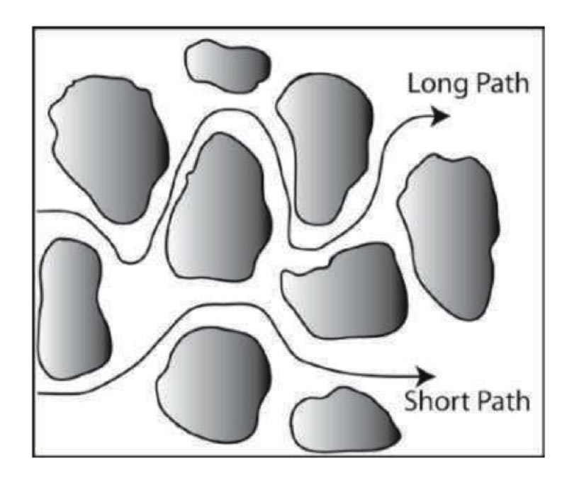
6.4 Dispersion
Dispersion describes the mixing of a solute due to fluctuations around the average velocity. This is caused by three factors: 1) microscopic heterogeneity, which make the fluid moves faster at the center of the pore and slower at the water grain boundary; 2) variations in pore sizes, in which cases fluid particles will move through larger pores faster; 3) variations in path length, causing some fluid particles going longer paths than others.
Mechanical Dispersion
Mechanical dispersion is a result of variations in flow velocities. Dispersion coefficients in porous media is typically defined as the product of the average fluid velocity and dispersivity $\alpha$:
where u is the average flow velocity (m/s) and $\alpha$ refers to the dispersivity (m). In systems with more than one direction, the longitudinal dispersivity DL in the principle flow direction is typically higher than DT in the direction transverse to the main flow.
Dispersion is a scale-dependent process with larger dispersivity values observed at larger spatial scales. At the column scale, a typical dispersivity may be on the order of centimeters. At the field scale, apparent dispersivities can vary from 10 to 100 m, as shown in Figure 2.
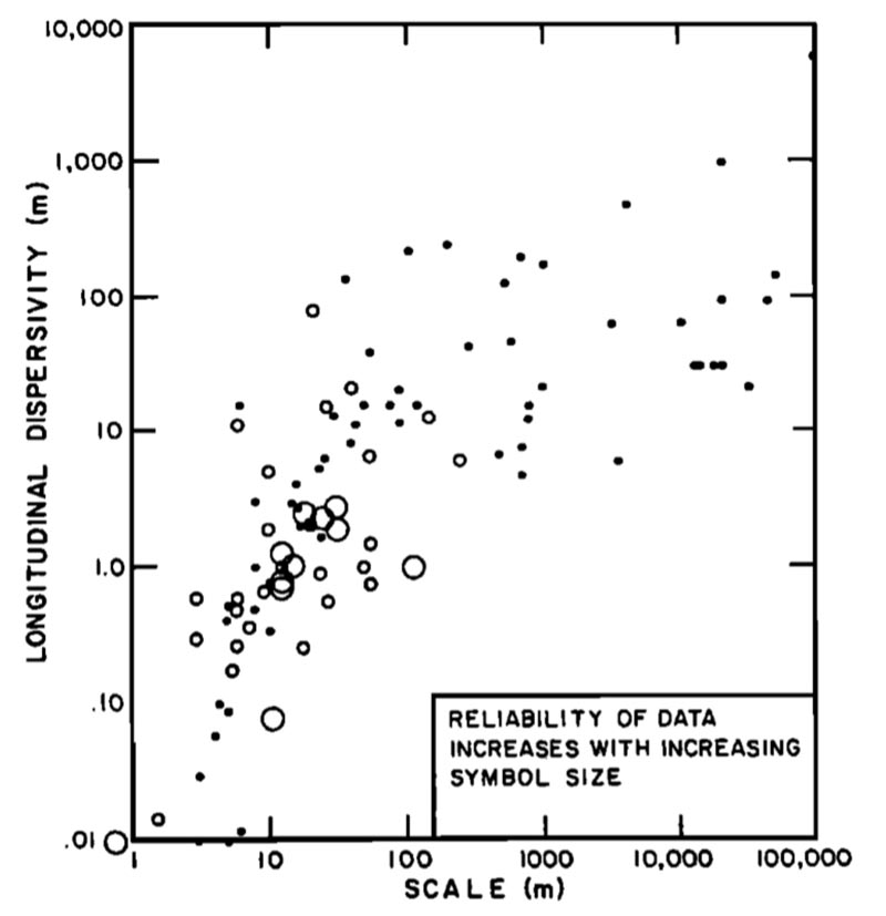
Hydrodynamic dispersion
The spreading of the solute mass as a result of diffusion and dispersion is similar to diffusion. This has led to the use of Fick’s First Law to describe the dispersion process as follows:
where Dh is the hydrodynamic dispersion coefficient defined as the sum of effective diffusion coefficient De and mechanical dispersion coefficient Dm:
As such, the hydrodynamic dispersion includes both diffusion and mechanical dispersion processes.
6.5 Advection Dispersion Equation (ADE)
By combining the transport processes outlined above, we can derive an expression for the mass conservation of a non-reactive solute as follows:
Substitution of Eqn. (1) and (13) into Eqn. (16) yields
Equation (17) is the classical Advection-Dispersion equation (ADE). For one-dimensional systems, Equation (17) is simplified into
Analytical solution of ADE is available for homogeneous porous media [Zheng and Bennett, 2002]:
with the initial and boundary conditions:
where C0 is the injecting concentration of the tracer, and erfc(B) is complementary error function:
6.6 Dimensionless numbers
Péclet number (Pe) is often used to describe the relative importance of advection and dispersion/diffusion in terms of their respective time scales $\tau_{a} \text { and } \tau_{d}$:
where L is the length of the domain of interest (m), u is the average Darcy flow velocity in the direction of interest (m/s), $D_{h}$ is the dynamic dispersion coefficient (m2/s). There are also some mathematical equations to define the time scales of these processes with similar concepts, mostly depending on the selected characteristic length [Elkhoury et al., 2013; Huysmans and Dassargues, 2005; Steefel and Maher, 2009; Szymczak and Ladd, 2009]. For example, L can also be the grid spacing (m) or correlation length (m) [Huysmans and Dassargues, 2005]. As shown in Figure 3, increasing Pe values indicate increasing dominance of advective transport and sharper front in breakthrough curves.
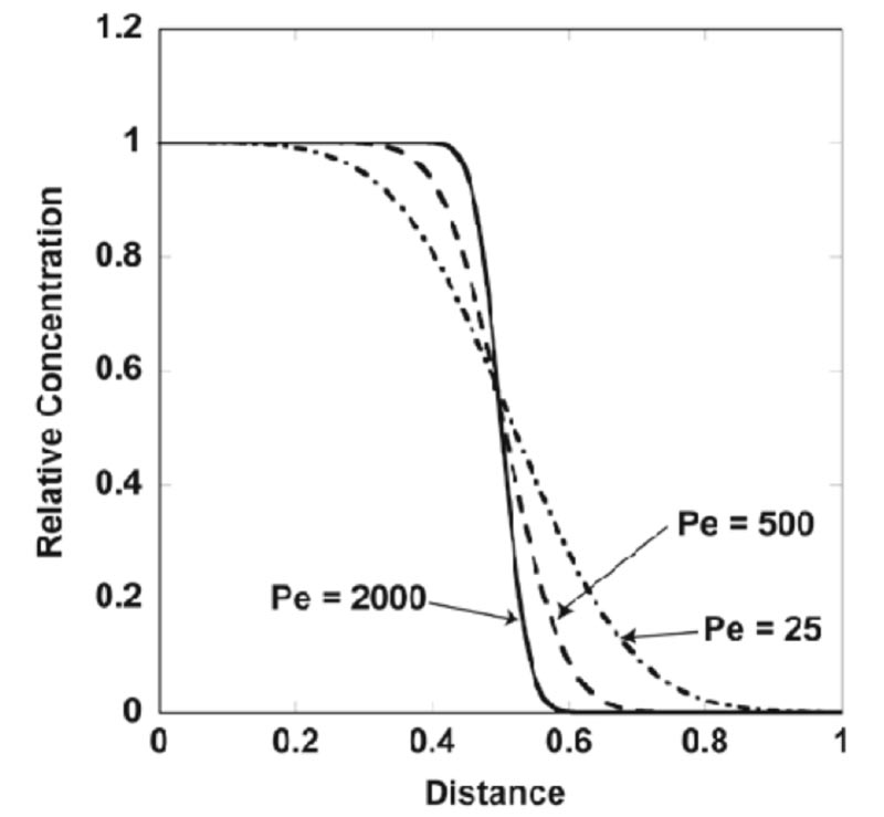
6.7 Setting Up 1D Flow and Transport Simulation in CrunchFlow
Please watch the following video: Advection-Dispersion Equation (ADE) for non-reactive tracers (16:42)
Click for a transcript of the ADE for non-reactive tracers video.
Advection-Dispersion Equation (ADE) for non-reactive tracers
So in is this video we'll be talking about advection-dispersion equation. This is first time actually we're not talking about chemistry but talking about the physical processes. So what do we have? Thinking about this is, let's say you have chemicals that are nonreactive. So the system you have we could use it as example is a column. So think about, for example, you are doing an experiment. You pack up a column, a column with like sand grains. And then you inject a chemical, let's say bromide, from the left into the right. So essentially you would have these chemical species you inject for a short period of time. You can imagine this is chemical will be moving along with the flow. So over time it will be eventually moving out of system with certain velocities. So v is the velocity here. And you are talking about here for example is the last of this column is L. So we want to know, as you can imagine, the constitution of this chemical would change with time and with space. Depends on what time you're looking at the snapshot. This chemical species might be here, might be here and other places there's no of this chemical species because we consider maybe, for example, we start with clean water.
So how do we mathematically solve this kind of equation and get the solution so we know the concentration of this chemical species in different time and different locations? And this is what we are going to talk about which is the advection-dispersion equation. We call it ADE with the other reaction terms. So ADE, when we think about it, I'm not going to derive in detail of where is this equation coming from. In general these equations are coming from these mass conservation principles. So if we look at these terms, different terms of the ADE, so the first home that we called the mass accumulation term. And it should have the units of accumulation, like mass per time. It's how fast things are changing. And this C is the concentration of the chemical species in the water phase. So C here is concentration of this-- let's call that tracer in water So everything we are solving is for how much they have in the water because that's what we really care about. And this should have the units of, for example, mass per volume.
So the first term is the mass accumulation. The second term here we call advective transport. So this is a process where there's a chemical almost you think about swimming. The chemical is a tracer. It actually flows together with the water at the same speed as the water flow. So that's called advective transport. And the last term is a dispersive transport. It's somewhat similar to diffusion process. It's driven by, first of all, concentration gradient, but also in this type of medias. You have grains. They tend to have different grain size, like different size of pore space and some spatial [INAUDIBLE] that leads to different flow velocity, mixing processes that lead to the concentration difference in different places. So these are three major terms in this equation. And for phi-- so this is phi is we call porosity, is how much space you have, how much pore space you have in a given volume. So the porous media has both pore space and solid space. So this is how much pore space in terms of percentage, per unit of total volume.
This v is velocity, flow velocity. It's a linear velocity in the pore space. So it's different from the u. We usually we call that's the velocity. And the relationship between the two, typically we knows that-- velocity-- we know that u will be equal to 5 porosity times the linear velocity. So there's a relationship between the two. And this Dh-- Dh is a very important term for this dispersive transport. This would be equal to-- I talk about it could be coming both from diffusion and the mechanical dispersion in porous media. So we have this kind of two terms adding together. This is coming from diffusion in porous media-- diffusion coefficient in porous media. And then the second term is essentially taking into account the mechanical dispersion. And you can think about alpha is called dispersivity, which is a parameter to describe how fast mechanical dispersion happens. And it's related to velocity. The whole term is also related to the velocity. So the flow, you actually have larger term of this.
So we have this equation. All the terms are here. And usually when this equation, there's an analytical solution for this equation if you give the right initial boundary condition. When we're numerically solving this, we will be discrete sizes of this equation in time and space, and then you get a solution for that. But before we do that, typical we need two conditions, right? This is the first time we introduced a space diminishing, x here. Before in the mineral dispersion precipitation, last time we actually induced the time. So you'll notice here that this equation, we call this is a partial differential equation, meaning it has two independent variables. One is the time. The other is space. So this is first time we introduce a space dimension here.
Now in order to solve this equation we need to know, like at t equal to 0, what are the concentrations? So this is initial condition. When t equal to 0, what are the concentrations? Now usually this is given for a given system. And we also need to know at the two boundaries, x equal to 0, x equal to L, what are the conditions that is specified? Is it, for example, a no-flow boundary or pure advective, or pure dispersive? These are different types of boundary conditions you can specify. But you will need to, in both the initial condition boundary conditions, to solve this. And different types of condition will give you different solutions because it matters what is the concentration in the t equal to 0. If your already start with something high you will see a different concentration versus, for example, at t equal to 0 you have clean water.
So terms of a solution, let's assume we have done all this work to solve the equation. What do we expect to see after we solve this equation? So I'm talking about a system. I'll be using an example system. So you will be injecting kind of shot pulse of this chemical bromide into a system. So if you conceptually think about it, at t equal to 0 it's somewhere here. And let's say everywhere it started with clean water. So you will have, at some point here, let's say you have kind of a little bit smeared at other time. And as time goes on you will have more and more smeared, but going in the direction of flow and moving along and maybe become more. So total mass will remain the same, but at the end you will see kind of wider and wider over time and over a longer distance. So this is conceptually how you would think about this solution you expect to see. Now when we think about from mathematical term, let's draw this. After we solve it, let's see. We'll look at the concentration as a function of distance. And what do you expect to see at different time?
So first of all, let's say at initial time you probably would see something like this. And here you see a pulse of this chemical. So is t at about 0, maybe a little bit past 0. But you think about, OK, over time, this pulse will move along. And then you should see different distributions. So this would be, let's say, at t equal to v times some small consolation, tu with C at another place. But this will become a little bit wider, smeared out. This is t1. And over time as you're going further distance, this becomes like more and more smooth. And I'm not drawing accurate. So total mass will remain the same. And I don't think I'm drawing nicely in terms of mass conservation. But in any case you will see over time total mass remain the same. But then the center of this will move along. So it's a v. So if it's a speed of this plume, how fast it moves over a certain time will be determined by-- so speed, v determines the speed of the center, of the rate of the center moving to downstream. But also another case will be-- we notice this Dh, which is a very important parameter as well. So if you're think about two different situations, let's say they both have the same v, but they will have different Dh values. Let's say we have another case with much higher Dh. Your will probably see something like this, a wider distribution. Still the same total mass, but it's much more spread. So this will be representing your large-- I'm sorry, a small Dh. The blue one would be representing a much larger Dh.
So now I draw the Dh. It will be more spread. So essentially you can think about Dh determines the width of the plume. So this is t1, t2. And over time, for example, if there's a t3 we care about, it should be even more spread out. This is t3. So if we wait long enough, this is going to spread a lot. So that's the type of solution you would expect to see when you have pulse of injection of a tracer. Now I'm just very briefly mentioning the characteristic time. There are several times we think is important. Once is residence time. This is directly related to how fast the flow goes and how long it actually stays in this column, how long this tracer actually stays in this column. So this we call tau a is equal to porosity times the length over mu. Or you can just say L over v. This is residence time. Another time is how long it takes for the dispersion process to uniform the whole concentration field. So this is what we call tau d. It's related to dispersion. So it's L squared divided by Dh. You can almost think about this as like if it's not open system, it would be how long it takes for diffusion to uniform, to homogenize the whole concentration field. And then a lot of times we define this Peclet number is tau d over tau a. So it's a relative between these two time scales or the rate of flow versus the rate of dispersion. And this should have a unit of L u phi Dh. This is a dimensionless number. So these times will determine like how fast-- you will realize this are kind of grouping dimensionless numbers. The Peclet number will determine the relative importance of dispersion versus advection, which in homework I asked you to do some exercises under different conditions with different Peclet numbers.
Example 6.1: Setting up 1D Flow and Transport Simulation in CrunchFlow
Click here for Example 6.1 CrunchFlow file package [39]
This example introduces setting up numerical simulation of the flow and transport processes for a non-reactive tracer in a 1D column of 10 cm long. A tracer Br- is injected into the column at the concentration of 1.2×10⁻⁴ mol/L. The permeability of the column is 1.75×10⁻¹³ m2 and the porosity is 0.40. A constant differential pressure is imposed at the x direction and results in a Darcy flow velocity of 4.20×10⁻⁶ m/s. The molecular diffusion coefficient in water D0 for the tracer bromide is 1.8×10⁻⁹ m2/s (between that of F- and Cl- in Table 1). The cementation exponent m is 1.0. The dispersivity α is 0.07 cm. In order to keep consistent with the value of water viscosity provided in the CrunchTope original code, the water viscosity we applied here is 1.00×10⁻³ Pas at 20 0C.
- Before the numerical experiment:
- Calculate the pressure gradient for the Darcy flow velocity.
- Calculate the effective diffusion coefficient De, mechanical dispersion coefficient Dm, hydrodynamic dispersion coefficient Dh. Which term dominates in Dh?
- Calculate the characteristic time for advection (residence time) and for dispersion, and Pe number. Based on the Pe number, predict which term dominates during the transport process.
- Set up in CrunchFlow using 100 grid blocks and run the simulation:
- Plot the bromide breakthrough curve at the end of the column (C/C0, with C0 being the injection concentration) versus residence time.
Click for Solution
Click here for input and database file package [39]
-
For the 1-D flow, Darcy flow equation can be simplified to:
$u=-\frac{\kappa}{\mu} \nabla P$
Thus, $\nabla p=\frac{4.20 \times 10^{-6} \mathrm{~m} / \mathrm{s} \times 1.00 \times 10^{-4} \mathrm{~Pa} \cdot \mathrm{s}}{1.75 \times 10^{-13} \mathrm{~m}^{2}}=2.40 \times 10^{4} \mathrm{~Pa} / \mathrm{m}$
This means that for a 10 cm (0.1 m) column, the pressure difference between one end to the other end of the column should be 2.40E3 Pa. Note that in Crunchflow, the pressure units is Pascal. - $D_{e}=\frac{D_{0}}{F}=\phi^{m} D_{0}=T_{L} D_{0}$
So $D_{e}=0.4^{1.0} \times 1.8 \times 10^{-9} \mathrm{~m}^{2} / \mathrm{s}=7.2 \times 10^{-10} \mathrm{~m}^{2} / \mathrm{s}$
$\mathbf{D}_{m}=\alpha \cdot \mathbf{u}$
So $D_{m}=0.07 \times 10^{-2} \mathrm{~m} \times 4.20 \times 10^{-6} \mathrm{~m} / \mathrm{s}=2.94 \times 10^{-9} \mathrm{~m}^{2} / \mathrm{s}$
$D_{h}=D_{e}+D_{m}=\phi^{m} D_{0}+D_{m}$
So $D_{h}=3.66 \times 10^{-9} \mathrm{~m}^{2} / \mathrm{s} \text { and } D_{m} \text { dominates } D_{h}(80.3 \%)$. - Residence time:
$\tau_{a}=\frac{V_{\text {pore }}}{Q}=\frac{\phi L A}{u A}=\frac{\phi L}{u}=\phi \frac{L}{u}$
So $\tau_{a}=0.1 \mathrm{~m} / 4.20 \times 10^{-6} \mathrm{~m} / \mathrm{s} \times 0.4=9.524 \times 10^{3} s==0.110 d$
Characteristic time for hydrodynamic dispersion:
$\tau_{d}=\frac{L^{2}}{D_{h}}$
So $\tau_{d}=0.1^{2} \mathrm{~m}^{2} /\left(3.66 \times 10^{-9} \mathrm{~m}^{2} / \mathrm{s}\right)=759 h=31.6 d$
$P e=\frac{\tau_{d}}{\tau_{a}}=\frac{L u}{\phi D_{h}}$
So $P e=31.6 d / 0.110 d=287>>1$, advection process dominates transport.
CrunchFlow setup brief: This is the first time that we set up spatial dimension in CrunchFlow. Please read CrunchFlow manual the DISCRETIZATION key word block (page 46 – 47), INITIAL_CONDITION and BOUNDARY_CONDITION (page 72) as well as the TRANSPORT keyword block (page 72-75). The CrunchFlow exercise example 6 also teaches how to set up non-reactive tracer test.
Solution 2:
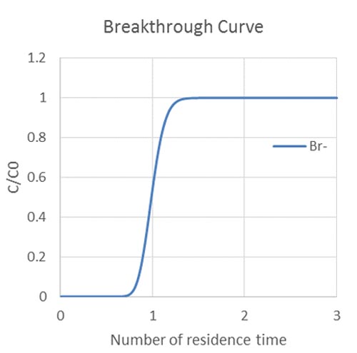
Figure 4. Breakthrough outlet concentration of Br- as a function of number of residence time. C0 is the initial injecting concentration of the tracer Br- while C is the tracer concentration at the outlet.
6.8 Homework Assignment
Assignment
- (60 points) As an extension of the in-class example, we will do another tracer test that only inject the tracer for the first 1/10 of the residence time. The rest of the time we will inject clean water into the column. Please note that in order to do this you will need to generate two input files with one inputfile having the keywords "restart", "save_restart", and "later_inputfile". Please read the relevant section in CrunchFlow manual for these keywords. The exercise 12 in the exercise folder has sample input files on using these key words.
- 1.1 Please plot the spatial profile of the tracer (concentration as a function of distance) at 1/10, 2/10, 4/10, and 8/10 of the residence time. Please plot all spatial profiles in one figure. Describe how the shapes of the Br concentration curve change over time. What causes that change?
- 1.2 Change the dispersvity $\alpha$ to 0.1 and 10.0 of the base value in example 6.1. Rerun these two additional simulations. And do the same plot as in question 1). Observe the difference in the shape of Br- concentration spatial profile with different $\alpha$ values. What are the effects of changing $\alpha$ values?
- (optional) (60 bonus points) As an extension of the in class example with continuous injection of Br- from the inlet, we will do a sensitivity analysis to understand the effect of parameters on the breakthrough curves in the same 1D column, including flow velocity, dispersivity, molecular diffusion coefficient, and cementation factor. In each sub question below, only one parameter or condition is changed. For each condition, please
- 2.1 calculate the characteristic times (residence time and dispersion time) and Pe;
- 2.2 draw the Br breakthrough curves (as a function of residence time) by changing only the parameter discussed in each sub-question, with all other parameters remaining the same as those in example 1. Note that each middle number is the number used in example 6.1 so you do not need to run the simulation again.
- flow velocity: 0.5, 1.0, and 2.0 of the flow velocity in example 6.1. Plot all three BTC in one figure and describe the effect of flow velocity on breakthrough curves (BTCs).
- dispersvity $\alpha$ : 0.1, 1.0, and 10.0 of the base value in example 6.1. Plot all three BTCs in one figure and describe the effects of dispersivity on BTC.
- Molecular diffusion D0: 0.1, 1.0, and 10.0 of the base value in example 6.1. Plot all three BTCs in one figure and describe the effect of D0 on BTC.
- cementation factor m: 1.0, 3.0, 5.0 of the base value in example 6.1. Plot all three BTC in one figure and describe the effect of cementation factor on BTC.
- compile all previous cases in 1) – 4) and make a table that lists values of residence time $\tau_a$, dispersion time $\tau_d$, De, Dm, Dh, v, and Pe. Plot all breakthrough curves together, label the Pe values for different cases in different ranges. What do you observe and why?
6.9 Summary and Final Tasks
Summary
In this lesson, we covered definition and principles of transport processes including advection, diffusion, and dispersion processes. We also discussed the Advection-Dispersion-Equation (ADE), its analytical solution, and how to set up solving ADE in CrunchFlow.
Other Relevant Textbooks:
-
Flow and Transport in Porous Formations (1989) by Gedeon Dagan;
-
Dynamics of fluids in porous media (2013) by Jacob Bear, Courier Dover Publications;
-
Applied contaminant transport modeling (2002), 2nd edition, by Chunmiao Zheng and Gordon D. Bennett, John Wiley and Sons, Inc.
References
Bear, J. (2013), Dynamics of fluids in porous media, Courier Dover Publications.
Brunet, J. P. L., L. Li, Z. T. Karpyn, B. G. Kutchko, B. Strazisar, and G. Bromhal (2013), Dynamic Evolution of Cement Composition and Transport Properties under Conditions Relevant to Geological Carbon Sequestration, Energy & Fuels, 27(8), 4208-4220.
Dullien, F. A. (1991), Porous media: fluid transport and pore structure, Academic press.
Elkhoury, J. E., P. Ameli, and R. L. Detwiler (2013), Dissolution and deformation in fractured carbonates caused by flow of CO< sub> 2</sub>-rich brine under reservoir conditions, International Journal of Greenhouse Gas Control, 16, S203-S215.
Gelhar, L. W. (1986), Stochastic subsurface hydrology from theory to applications, Water Resour Res, 22(9S), 135S-145S.
Haynes, W. M. (2012), CRC handbook of chemistry and physics, CRC press.
Huysmans, M., and A. Dassargues (2005), Review of the use of Péclet numbers to determine the relative importance of advection and diffusion in low permeability environments, Hydrogeol J, 13(5-6), 895-904.
Oelkers, E. H. (1996), Physical and chemical properties of rocks and fluids for chemical mass transport calculations, Reviews in Mineralogy and Geochemistry, 34(1), 131-191.
Steefel, C. I., and K. Maher (2009), Fluid-Rock Interaction: A Reactive Transport Approach, Rev Mineral Geochem, 70, 485-532.
Steefel, C. I., D. J. DePaolo, and P. C. Lichtner (2005), Reactive transport modeling: An essential tool and a new research approach for the Earth sciences, Earth Planet Sc Lett, 240(3-4), 539-558.
Szymczak, P., and A. J. C. Ladd (2009), Wormhole formation in dissolving fractures, J Geophys Res-Sol Ea, 114.
Zheng, C., and G. D. Bennett (2002), Applied contaminant transport modeling: theory and practice, 2nd ed., 621 pp., John Wiley and Sons, Inc., New York.
Lesson 8: Flow and Transport Processes in 2D Heterogeneous Porous Media
Overview
This unit introduces general concepts of spatial heterogeneities, principles of physical flow and transport processes in heterogeneous porous media, as well as how to set up simulations for flow and non-reactive transport in a 2D heterogeneous domain in CrunchFlow.
Learning Outcomes
By the end of this lesson, you should be able to:
- Understand fundamental principles and geostatistical measures of spatial heterogeneities
- Set up flow and transport simulation in 2D heterogeneous porous medium domain in CrunchFlow
Lesson Roadmap
| Recommended Readings |
|
|---|---|
| To Do |
|
Questions?
If you have any questions, please post them to our Questions? discussion forum (not e-mail), located in Canvas. The TA and I will check that discussion forum daily to respond. While you are there, feel free to post your own responses if you, too, are able to help out a classmate.
8.1 Flow and Transport in Multiple Dimensions
Flow and transport processes, including advection, dispersion and diffusion are described in the lesson Flow and Transport Processes in 1D System. In natural system we often need to consider these processes in multiple dimensions and in heterogeneous systems where the physical and geochemical properties of the subsurface are not evenly distributed. As an example, in Figure 1, we show that the distribution of permeability dictates the spatial distribution of injected tracer from injection wells during a biostimulation experiments at Old Rifle, Colorado (Li et al., 2010).
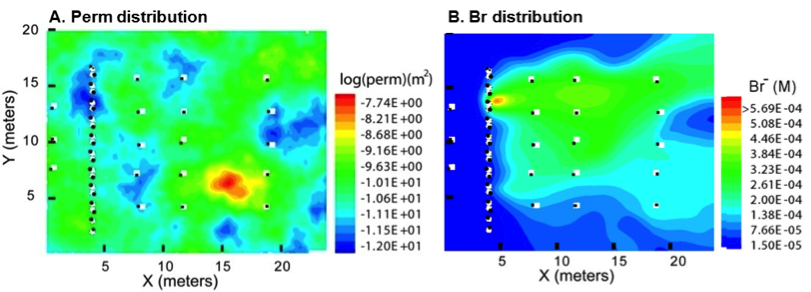
The general Advection-Dispersion Equation (ADE) in multiple dimensions is as follows:
Here C is the tracer concentration (mol/m3 pore volume), t is time (s), D is the combined dispersion–diffusion tensor (m2/s), v (m/s) is the flow velocity vector and can be decomposed into vL and vT in the directions longitudinal and transverse to the main flow in a 2D system. The dispersion-diffusion tensor D is defined as the sum of the mechanical dispersion coefficient and the effective diffusion coefficient in porous media De(m2/s). At any particular location (grid block), their corresponding diffusion / dispersion coefficients DL (m2/s) and DT (m2/s) are calculated as follows:
Here $\alpha_L$ and $\alpha_T$ are the longitudinal and transverse dispersivity (m). The dispersion coefficients vary spatially due to the non-uniform permeability distribution. Values of $\alpha_T$ are typically at least one order of magnitude smaller than $\alpha_L$ (Gelhar et al., 1992; Olsson and Grathwohl, 2007).
8.2 Homogeneity vs. Heterogeneity
The terms homogeneity and heterogeneity are used to describe the uniformity and regularity in spatial distribution of geomaterial properties in natural subsurface systems. Homogeneity means spatially uniform-distributed properties. In natural systems, geological media are almost always heterogeneous. That is, their physical and (bio)geochemical properties vary spatially. Spatial heterogeneity can refer to both physical and geochemical properties. Physical properties include mineral grain size, porosity, and permeability / conductivity. Geochemical properties include, for example, mineral types, lithology, mineral surface area, and cation exchange capacity. Figure 2 shows a picture of an outcrop with layers of different types of geomaterials from the Macrodispersion site (MADE) in Columbia, Mississippi (Zheng and Gorelick, 2003).
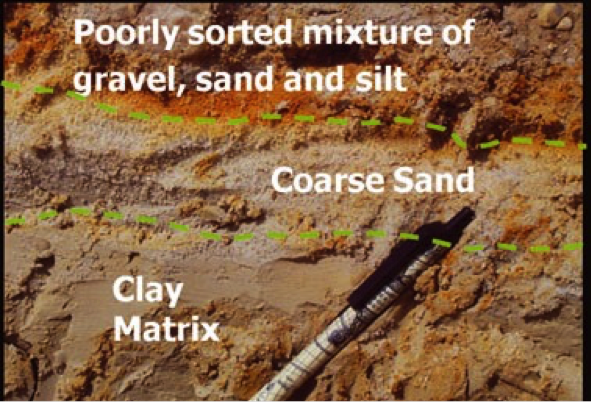
Spatial heterogeneities can lead to significantly different chemical reactions and physical transport processes from their homogeneous counterparts. As a result, heterogeneities play an important role in determining processes and applications in subsurface systems. Examples include contaminant reactive transport (Li et al., 2011), oil and gas production (Chen et al., 2014; Hewett, 1986), and environmental bioremediation (Murphy et al., 1997; Song et al., 2014). For example, as shown in Figure 3, the different geomaterials in Figure 2 leads to orders of magnitude in the spatial variation of hydraulic conductivity (Figure 3A), and abnormal solute transport (Figure 3B) (Zheng et al., 2011).
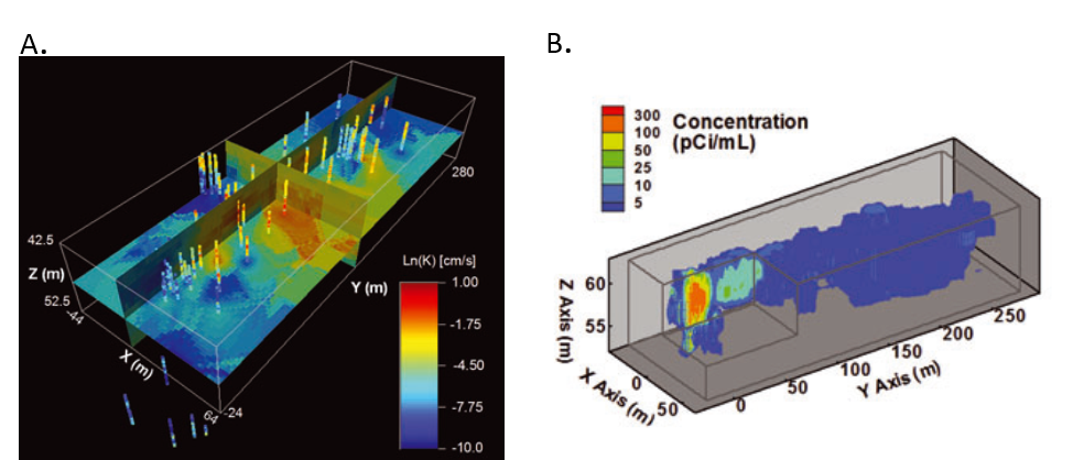
8.3 Quantitative Measures of Spatial Heterogeneity
Geostatistics has been well developed to quantitatively describe the characteristics of spatial physical heterogeneities, especially conductivity / permeability, in the natural subsurface. Here we briefly introduce a few geostatistical measures. Interested readers are referred to geostatistical books and software tools for more detailed information (Deutsch and Journel, 1992; Remy and Wu., 2009).
Mean of permeability
It measures the average water-conducting capability of porous media. There are different definitions widely used in subsurface hydrology:
Arithmetic mean $\kappa_T$ is defined as:
Here n is the total number of zones or subsystems; $\kappa_i$ is the local permeability of subsystem.
Harmonic mean $\kappa_h$ is defined as:
Geometric mean $\kappa_g$ is defined as:
Effective permeability$\kappa_e$ is derived from the Darcy’s Law:
where u is the average flow velocity (m/s) of the field; $\mu$ is the flow viscosity (Pa·s); $\Delta L$ is the length (m) along the main flow direction; $\Delta P$ is the pressure differential (Pa) along the main flow direction. The effective permeability describes the real water-conducting capability of the porous media. The upper bound of the effective permeability is often the arithmetic mean, and the lower bound is the harmonic mean. They correspond to flow through a perfectly layered systems, parallel and perpendicular to the layering, respectively (Heidari and Li, 2014; Zinn and Harvey, 2003).
Variance of permeability
The extent of deviation from the mean is calculated as follows:
where $\operatorname{Var}(\kappa)$ is the permeability variance (m4). Larger variance indicates larger extent of spatial heterogeneity. Permeability of geological media differs significantly in natural subsurface systems. Conductivity (K) is also commonly used as a measure of conducting capability of porous media. The Macrodispersion Experiment (MADE) site in Mississippi has both small silt and sand regions. It has a centimeter scale ln(K) variance as large as 20, while its variance at the meter-scale measured by borehole flowmeters is approximately 4.0, which is considerably smaller because small-scale variability is averaged out (Feehley et al., 2000; Harvey and Gorelick, 2000; Zinn and Harvey, 2003). The Wilcox aquifer in Texas also has high ln(K) variance of about 10, as does the Livermore site (ln(K) variance >20) (Fogg, 1986; LaBolle and Fogg, 2002). The Bordon site at Borden, Ontario, however, is relatively homogeneous with ln(K) variance around 0.20 (Mackay et al., 1986; Sudicky, 1986). Note that ln(K) mentioned here is the natural logarithm of hydraulic conductivity K (m/s).
Correlation Length
Correlation length is a measure of correlation in spatial variation. Two points that are separated by a distance larger than the correlation length have fluctuations that are relatively independent, or uncorrelated. In contrast, properties of two points that are within correlation length are correlated. For detailed calculation and application of correlation length in subsurface fields, readers are referred to (Bruderer-Weng et al., 2004; Gelhar, 1986; Heidari and Li, 2014; Salamon et al., 2007). Correlation lengths differ significantly in natural subsurface systems, as shown in Table 1. Figure 4 shows the patterns of permeability fields (m2) with different correlation length generated from Gaussian Sequential Simulation Method.
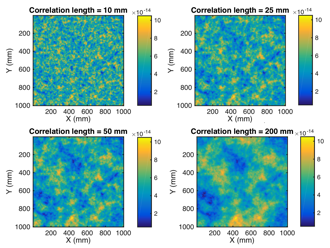
| Source | Geological Media | Correlation Length (m): Horizontal | Correlation Length (m): Vertical | Overall Length (m): Horizontal | Overall Length (m): Vertical |
|---|---|---|---|---|---|
| Socorro, New Mexico | fluvial sand | >3 | 0.1 | 14 | 5 |
| Rio Grande Valley, New Mexico | fluvial sand | 7.6 | 760 | ||
| Cape Cod, Massachusetts | glacial outwash sand | 5 | 0.26 | 20 | 5 |
| East central Illinois | sandstone aquifer | 4.5×10⁴ | -- | 5×10⁵ | -- |
| Las Vruces, New Mexico | alluvial silty-clay loam soil | 0.1 | -- | 6 | -- |
Hydraulic connectivity
A series of hydraulic connectivity have been defined as integrative measures of spatial heterogeneity characteristics. Static connectivity can be calculated by the connective structure of the hydraulic conductivity or geological facies. Dynamic connectivity directly relates to physical flow or transport processes. For interested readers, we refer them to (Knudby and Carrera, 2005; Knudby and Carrera, 2006; Renard and Allard, 2013; Siirila-Woodburn and Maxwell, 2014; Willmann et al., 2008).
8.4 Setting Up 2D Heterogeneous Domain and Transport Process in CrunchFlow
Setting up 2D heterogeneous domain for flow and transport calculation generally includes three primary steps. First, the 2D domain needs to be defined with the targeted size, dimension, and resolution. The relevant keyword blocks for setting up the domain include DISCRETIZATION, INITIAL_CONDITION, and BOUNDARY_CONDITION. The second step involves the set up for the calculation of flow, which involves the use of various keywords in the FLOW key block, including constant_flow, calculate_flow, read_permeabilityFile, and pressure. For 2D heterogeneous systems we always use “calculate_flow” to calculate flow by specifying a pressure gradient using “pressure” at the two main boundaries. The permeability distribution can be either defined in INITIAL_CONDITIONS with relevant permeability values in specific grid blocks defined under GEOCHEMICAL_CONDITIONS, or by reading in permeability distribution using the keyword read_permeabilityFile. Detailed format of the permeability file is provided in the manual. After that, the transport keywords can be specified in the TRANSPORT keyword block, similar to the ones discussed in the 1D homogeneous setup.
Example 8.1
Click here [41] for CrunchFlow Files for Example 8.1 and other related files for Li et al. 2014
The following gives an example of setting up flow and transport calculations in 2D homogeneous and heterogeneous domains. Here we use the physical set up of 2D cross-sections of the Mixed and One-zone column in (Li et al., 2014). The authors packed 4 columns of 2.5 cm in diameter and 10.0 cm in length with relatively similar amount of magnesite and quartz distributed in different spatial patterns. Here we focus on two columns that represent two extreme cases: the Mixed column with uniform distributed magnesite and quartz, as well as the One-zone column with magnesite all gathered in one cylindrical zone of diameter of 1.0 centimeter. To keep it simple, here we will do the calculation for 2D cross-sections, instead of following the steps in section 3.2.4 in the paper to convert 2D to 3D. So our numbers might be different from the paper. We are also assuming that in the middle one zone magnesite is 100% of the solid phase. The 2D system has a size of 25 mm by 100 mm. A constant differential pressure is imposed at the boundaries in the z (vertical) direction, leading the primary water flow direction in the z direction from the bottom to the top. No flux boundaries are specified in the X direction (Li et al., 2014).
| Columns | Mg zone |
Qtz zone | $^2a_L$ (cm) |
$^4a_T$ (cm) |
$\mathrm{\kappa}_e$ (×10-13m2) |
$\phi_{\mathrm{avg}}$ |
|---|---|---|---|---|---|---|
| Mixed | 0.05 | 0.005 | 8.26 | 0.44 | ||
| One-zone | Width: 1.0 cm
$\Phi_{Mg:}\ 0.54$ |
Width: 1.5 cm $\Phi _{Qtz:}\ 0.38$ |
0.07 | 0.004 | 10.74 | 0.44 |
*The permeability of the pure sand columns of the same grain size was measured to be $8.7 \times 10^{-13} \mathrm{~m}^{2}$.
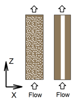
Please do the following:
- Given the effective permeability of the One-zone column and the pure sand column, calculate the permeability of the magnesite zone based on the arithmetic average of the equation;
- Calculate the volume fraction of the magnesite and quartz assuming the two columns have the same total mass and volume fraction of magnesite and quartz;
- Following descriptions in Li et al. (2014) Fig. 1, calculate the pressure field needed for each column in order to have a flow velocity of 3.6 m/day;
- What is the residence time when the flow velocity is 3.6 m/day?
Run the simulation at the grid block resolution of 1 mm by 1 mm.
- Generate the flow field of the two columns. What is flow velocity in the homogeneous column? What is the flow velocity in the magnesite and sand zone of the One-zone column? What is the ratio of the flow velocity between the two zones? Are they consistent with the permeability ratio of the two zones?
- If we inject Br at the concentration of 1.2×10⁻⁴ mol/L at the inlet, please generate the bromide breakthrough curves for the two columns. Note that here you will assume that you only one outlet that integrate all the flow and concentration coming out the outlet grid blocks using the equation
\begin{equation}C_{a v g}=\sum_{i=1}^{n} C_{i} q_{i} / \sum_{i=1}^{n} q_{i}\end{equation}where Ci and qi are the concentration and flow rate from the grid block i in the outlet cross-section. Please plot the overall breakthrough curves from the two columns and discuss their differences.
Note: in plotting 2D figures, you can use softwares such as Tecplot or Matlab. Penn State provides free Matlab web access on WebLabs at Penn State [42]. You can access matlab from there. In addition, you can also get video tutorials from LinkedInLearning [43] at Penn State about using matlab.
Lesson 8 - Mixed 2D.1 Video (56:05 minutes)
Li Li: All right, so this is the video for lesson eight, continued. We just finished doing the homogeneous column. 2D, we call that-- mixed 2D. So you should have watched that first, before you start this one, because the other one has a lot of backdoor information that I provided.
And on top of that, we made the mistake of missing that keyword, zone, in specified permeability. So hopefully, that helps you remember. This is very important.
And then, you have-- I guess, that's the value of making mistakes from my side. And then, you see how things are fixed, and all that. So here, we are going to-- in this one, I'm going to talk about how to do the one zone case. And again, we'll be specifying all the different keyword blocks starting from specify the domain, and then flow, and then transport, and then the reaction-- and then, the initial condition, boundary condition, and all that. So it will be followed in order.
And first, let's also start with discretization. And again, we're using 25 by 100 grid blocks-- 2,500 grid blocks. So essentially, you would have the same discretization. For example, just like what we did before for the homogeneous case-- distance_units. And you would have millimeters. And then, you have xzones-- 25 and space in 1.0 millimeter. Y zones-- you have 100, again 1.0 millimeter as a space.
And then, you are going to specify your domain. But now, we can not specify porosity directly, because there's average porosity, but there's also porosity in different zones, as they are different. The middle zone it's magnesite. The offsite zone is quartz.
And they have different porosity. So we are now going to specify fixed porosity. So here, we are going to just do a porosity update, whatever it is.
And then, we do need to specify the minerals, because different minerals are your different parts of the column. So you actually need magnesite. You also need quartz. And then, you will be specifying different mineral in different parts of the column.
So let's do flow first, just like what we did before, because you do need to calculate its flow, for the flow units are all-- everything you need to calculate the flow field. So again, we are doing time units being seconds. And then, you have distance units being meters. And then, you have calculate flow, true.
So then, you will be specifying permeability. So when you specify permeability, when you do default, you do need to really specify your zone. So I'm going to specify for everything to be 8.74E-13, which is a permeability of the cross-zone first. So when I do default, that means a whole domain have this permeability.
Why do I do that? Because then, I don't need to specify separately. Later on, we'll override. I will specify the magnesite side part, and then override that. So this is the permeability of-- you can specify for the whole domain default. You don't specify zones.
But then I write, later on, permeability_x for the magnesite zone. We calculate that in that, before they're doing this simulation. It's for the middle zone, right? So you have one centimeter with magnesite zone in the middle, and then 0.75 choosing the two other side there.
So into my grid blocks, you would have 8 to 18. Fluctuation, be 9 to 18, is-- sorry-- is the middle magnesite zone.
You would also have this. 13 points-- so that's for the magnesite. Or this would be y. So that specifies the magnesite zone permeability.
OK, so by doing that-- so first of all, here, I specify everywhere is have this value. Now, later, I specify in these zones, you would have these values. So this part of a zone will be overwritten by these values. And the original ones that is not specified is going to remain the same. So you still have-- quartz zone have this value, but the middle of magnesite is going to be overwritten by these values.
And then again, we're going to specify permeability_x like the no-flow boundaries. And you would have zone 0-0, 26-26, as these other ghost cells from-- I'm sorry, 0-0, 1-100, 1-1. And they are permeability_x, 0. And then, again, this zone is very important-- 26, 26.
Actually, I might made a mistake in the previous [INAUDIBLE]. It should be-- really it's a ghost cell outside of the grid block one for x, grid block 25 for x, because these are the no-flow boundary. Again, this will be no flow. So if I made a mistake, make sure you know that was a mistake-- no-flow boundary.
All right, that's permeability. And then, we need to specify pressure. Now see, again, we put the value upon one everywhere. This doesn't really matter. The code we essentially use Darcy's Law given the heterogeneous distribution of permeability and then discretization. So whatever initial value is going to be erased, but we don't want to leave it undefined.
Pressure in that will be 3890. We do the calculation in that before we do the simulation. But again, specified zone will be in the 1-25 in the ghost cell just before you have grid block one. One fix, and then you have pressure, zero again. Zone 1-25-- that's the x. And then, y is 101-101 fix.
So that's a flow. So you are supposed to have everything you need to calculate the flow field. Then, let's look at transport.
Transport will be very similar to what we had before. We need all these dispersion diffusion-related distance units, again, with the centimeters. Time units-- seconds. And then, I'm going to do the same fix diffusion as what we did in the previous one-- 6.342E-6. And then, you have cementation exponent-- cementation, dispersivity.
Dispersivity-- again, the first one is for x, and the second one is for y. So according to the number in the table, you have 0.004, 0.07 centimeters for the two dispersivities. So that's for the transport. And then we need to specify [INAUDIBLE] of the column. Now in here, you have two different zones. One is quart zone. The other is magnesite zone. So we actually specify the two minerals. First of all, we need to specify the primary species.
Now I talk about before, this is a tracer test. So we definitely would need bromide. But also [INAUDIBLE] you put different minerals, you need all the elements, building blocks for that mineral. So for magnesite, you need Mg2 plus because it's MgCO3, so you also need CO2 aq. You need carbonate species.
For quartz, you would need the aqueous species SiO2 aq. But also it is in water. So let's just put H plus there. Just in case some [INAUDIBLE], for example, magnesite is written in terms of H plus. And then second species, you will need OH minus. These species don't really matter in the tracer test. But it will be important later on. But since we are going to specify different mineral zones, even where only for physical process, we do need all the chemical building blocks.
So CO2 aq, then you need bicarbonate, carbonate species. I believe that's it. So these are primary species. And then you need to specify your inlet. Let's just copy all the primary species then, because we know we need that. Inlet, just like what we had before. Units, let's still do molar. Just to be consistent, let's still do molar.
Temperature, bromide, OK, inlet, you have bromide concentration of 1.210 e minus 4. Magnesium, we consider this clean water. So let's just put very low concentration there. Here we also put very low concentration in SiO2, we have low concentration. Because this doesn't really matter at this point. And maybe we put a pH of 7.0. Shouldn't really matter because it's not going to calculate that much anyway.
So for the condition, in the column we have quartz zone and we have magnesite zone. So essentially, we will need both of these. And then primary species, this would be initial in the quartz part. So let's see, still do low concentration bromide. But here, notice these are specified in the aqueous phase. Now we are also going to specify the solid phase.
And for quartz zone, we talk about the positive quartz zone is 0.38. So that means the solid phase is 0.62. So you would have quartz is essentially volume fraction of 0.62. And you put magnesite because you don't have magnesite there. You are going to put very low value.
So essentially, that will give you-- the code will calculate, OK, you have this much solids with a total solid phase of 0.62, then you will calculate porosity being 0.38. I'm just making notes here.
So for magnesite zone, we will still having the whole thing accept the solid phase is different. Because for magnesite, you still have initial condition, that much of these species. But now your quartz will be very small number.
And then your magnesite, remember your magnesite porosity is 0.54. So your magnesite mole volume fraction should be 0.46. So that adding up to be 1. You have the different conditions, just to avoid confusion. So that's the three conditions-- inlet, quartz, magnesite.
Let's specify for the initial conditions. At first, let's specify the whole domain. So there is more quartz [INAUDIBLE] let's specify the whole domain being quartz. So you're putting like one to 25, and then 1 to 100, [INAUDIBLE] for quartz. So that's saying, everywhere you have quartz.
But then, I'm going to override that, the middle part which is nine to 18 will be the magnesite. We're taking the magnesite initial conditions. So that's it gives you, specify initial condition. Then we need a boundary condition. Where is boundary condition?
For the boundary condition, it will be very similar, x_begin, y_begin, x would be inlet. And then you have flux. x_end. Let's say you will do quartz. It doesn't matter much. It's inlet that it is important. And y_begin, y_end. So again, it will take whatever it is coming out of the column. It shouldn't really matter. Boundary condition.
And then you have output. Again, you need to specify how frequently you want things to-- how long do you want to run, how frequent you want output, where do you want output. Spatial profiles, specify, let's do it the same as what we had before-- 0.0011, 0.1, 0.15, and maybe then 0.2. So run the same time as the previous one.
And let's do the time series output, maybe also for the middle. But if you want to look at every outlet block, you're welcome to do that. You don't have to have only one.
For example, you can specify 25 different time series for all the alternate block. Let's say I'm just doing another one time series. Breakthrough, let's say I'm looking at 20. And then [INAUDIBLE] 20, 100, 1. So now you have two different groups. You're looking at the 13 square blocks in the outlet cross section and then 20 square blocks in the outlet.
And then you will be output since this is tracer test. So all that matters to us is bromide. And then we have times series interval should be whatever, 4, 10, or whatever works. All right.
So that seems all we have. Just kind of quickly looking through. I usually try to be clear about what I put in and what are keywords and not making it too crowded. So I'm going to separate that because a lot of times it's easier to see. Line up boundary condition, transport, porosity, discretization, minerals.
For minerals, it's important that you realize that for the name of the minerals, you need the capital in the first letter. Otherwise, the code doesn't recognize it. And then flow, and then you define all the calculated flow, permitted value, permitted value, make sure I have all the zones there when I define specific zone for certain numbers. Zone, zone, OK.
All right. Primary species, secondary species, initial condition, quartz, magnesite. That's consistent always. Let me see. Initial condition, let me just make sure. Yeah, it's consistent with [? permitted that I ?] set up.
Condition inlet, you're putting high concentration bromide and then condition quartz, condition magnesite. You're putting specific volume fraction quartz in various fraction of magnesite, for them to be adding up to be 1 with porosity. All right. So it looks like all right. Let's try it.
So it looks like it's taking this in. And we didn't make mistake again this time, which is good. So first timestamp, it spit it out. And I want to point you to the velocity. So the reasons there's velocity and velocity evolved is because I'm putting porosity to update. So the code will try to update the porosity, although there's no reaction going on or anything. But that's fine.
And then you have porosity. So let's look at velocity. You will realize the velocity is different for different zones, as you can see. And that's more or less because we have different-- permitting different zone. So for this 2D, you will need either product. So spatial profile in 2D like [? Techprod ?] or Matlab, whatever software you use.
The x velocity is not very meaningful. So I would say you just plot the y velocity, which is in direction of the flow. And you realize, OK, y is 1.07. They all have the same units. You're going to go back and check with the corresponding [INAUDIBLE] But in any case, this is 1.07. This is 1.68. Because we just have two zones. And you could imagine this would be the one in the middle zones. And magnesite has a little bit higher probability.
In any case, if you divide 1.68 to 1.07, you get about 1.6 or something. And you realize that when you put the input file, the permitted value of the magnesite is about 1.6 times of the quartz zone. So essentially, the flow is distributed according to the permitted values.
And if you [INAUDIBLE] it should come up with, for example, flow velocity distribution somewhat like the figure one that are we showed with different flow velocity and everything in different places. It's still calculating. It seems really slow for some reason. It's to the 6.35 times 10 to minus 2. OK, still have a bit of time to go.
Because we have more species. And even though we don't really care about these species, we just have to put them there. And the code will try to calculate everything, I'm sure. So it's slower than the homogeneous column.
But in any case, the breakthrough, so for the velocity-- and actually for even let's look at total concentration. So you have x and y. And then you have all different species. But all your K is bromide. So you will be looking at, there's a third column. When you try to calculate the overall breakthrough, imagine you have the 2D. And then in each of the grid block in outlet, you have, for example, let me just go back. It's probably easier to explain with a figure.
This really should be x and y, not x and z. I will change that. In any case, this is your x direction. And this is your y direction. So the [INAUDIBLE] will come out flow velocity different when y equal to 100. This will be y equal to 1, y equal to 100. And this is x.
So you will have different flow velocity coming out from each of the outlet grid blocks. You will also have different concentration coming out because of different [INAUDIBLE]. So what I'm asking you to do, for example, I'll specify a little bit, the concentration average, imagine when we take sample, we actually only have one outlet, not like everywhere you have a sampling point. So that one outlet is essentially integrating all the concentration and flow velocity out of it. So when you calculate average breakthrough, you actually use a flow rate weighted average to do the calculation.
So it would need to be like CI coming out from each of these times, VI and cross section I of each out of this. That way, you get flow rate times concentration, which is mass per time for integrating summation [INAUDIBLE] grid block and divided by the overall flow rate. That will give you the average breakthrough.
So what you need to do when you look at these would be you look at bromide. And you will be looking at y equal to 100. In the example, you get each value, the flow velocity. Cross section area is area of the grid block times porosity. Velocity times that cross section area times the concentration is what you get for each grid block. And then you add them up, divided by the overall flow rate. So that's what you are going to do when you do the breakthrough curve.
And you are going to see a bit of difference in the mix column and in the 2D column. I'm not going to tell you at this point. But in any case, this is what you are going to do. Now we're at 0.16. So we have a little bit. I think we specified to 0.2. So you still have a little bit of time to go. So that's total concentration.
Let me just leave it open. One more. The permitted will give you the distribution of the permitted in different parts of the grid block. These have the units of log 10 meters squared. So these are in log units.
Porosity, [INAUDIBLE] you have xy. And then you have porosity somewhere. For the magnesite zone, you have 54% porosity. And 38 is 38%. So these are the output files. Let me see. Rate, we're not really interested in that.
So it has velocity. If you do have [INAUDIBLE] dissolving out, it will be updating the porosity, permeability, and everything, according to the porosity-permeability relation in the code. And that actually will give you different distributional porosity and permeability from the initial values over time.
I think we are done. Everything is out. And all you need to do is plot thing out and look at the difference in the breakthrough curve, think about why they are different. And you would do-- be interesting to think about how they are different, why they are different, and all that. And I think this is the one zone example with heterogeneity. And you can specify all that.
There is another option. Let's see if you have kind of random distribution of permeability. We can specify in another separate file and [INAUDIBLE] code to read permeability for like irregularly shaped heterogeneity distribution. And this, we're not going to cover. It's a little bit too complicated for now.
So I'm going to stop here. And I'm sure you will have fun. It'll take a little bit more work. But it's also very interesting and very useful when you think about heterogeneity of system, how physical processes are different.
And later on, there will be another session. In Unit Three, we'll be taking about 2D reactive. So this is really building the physical process for that unit later on for the reactive one. All right. I'm going to stop here. I think this is a bit too long.
Solution
-
Effective permeability of the One-zone column:
$\kappa_{\text {eff-onezone }}=10.74 \times 10^{-13} \mathrm{m}^{2}$Pure sand column permeability:
$\kappa_{\text {sand }}=8.74 \times 10^{-13} \mathrm{m}^{2}$This indicates that the permeability of sand zone in the One-zone column is $8.74 \times 10^{-13} \mathrm{m}^{2}$. As the sand and magnesite zones are layered parallel to the flow direction, we can apply Equation (4) to solve the magnesite zone permeability:
$\kappa_{a}=\frac{1}{n} \sum_{i=1}^{n} \kappa_{i}$Here, the volume fraction for sand zone is:
$\left(D_{\text {column }}-D_{\text {magnesite-zone }}\right) / D_{\text {column }}=(2.5-1.0) \mathrm{cm} / 2.5 \mathrm{~cm}=0.6$The volume fraction for magnesite zone is:
$1-0.6=0.4$Hence,
$\begin{array}{l}\kappa_{\text{eff-onezone }}=0.6\kappa_{\text{sand-zone }}+0.4\kappa_{\text{magnesite-zone }}\\
\kappa_{\text{magnesite-zone }}=\frac{\kappa_{\text{eff-onezone }-0.6\kappa_{\text{sand-zone }}}}{0.4}\\
=\frac{10.74\times10^{-13}-0.6\times8.74\times10^{-13}}{0.4}\mathrm{m}^2\\
=13.74\times10^{-13}\mathrm{m}^2\end{array}$ -
In the One-zone column, the magnesite volume fraction = volume fraction of magnesite zone * $\left(1-f_{\mathrm{Mq}}\right)=0.4^{*}(1-0.54)=0.184$. In the Mixed column, the average porosity is 0.44 so the solid phase volume fraction is 0.56. The Mixed column should have the same total amount of magnesite volume as in One-zone column. Therefore The volume fraction of magneiste in the Mixed column = 0.184 and the volume fraction of quartz is the Mixed column = 0.56 – 0.184 = 0.376.
-
We can apply Darcy's Law, Equation (7) to calculate the pressure gradient:
$\kappa_{e}=\frac{u \mu \Delta L}{\Delta P}$Here,
$\begin{array}{l}
u=3.6 \mathrm{~m} / d a y=4.17 \times 10^{-5} \mathrm{m} / \mathrm{s} \\
\mu=1.002 \times 10^{-3} \mathrm{Pa} \cdot \mathrm{s} \\
\Delta L=10.0 \mathrm{~cm}=0.10 \mathrm{m}
\end{array}$For the Mixed column,
$\kappa_{e f f-m i x}=8.26 \times 10^{-13} \mathrm{m}^{2}$Hence,
$\begin{aligned}\Delta P_{\text{mix }}&=\frac{u\mu\Delta L}{\kappa_{\text{eff-mix }}}\\
&=\frac{4.17\times10^{-5}\times1.002\times10^{-3}\times0.10}{8.26\times10^{-13}}Pa\\
&=5.06\times10^3\mathrm{Pa}\end{aligned}$For the One-zone column,
$\kappa_{\text {eff-onezone }}=10.74 \times 10^{-13} \mathrm{m}^{2}$Hence,
$\begin{aligned}\Delta P_{\text{one-zone }}&=\frac{u\mu\Delta L}{\kappa_{\text{eff-onezone }}}\\
&=\frac{4.17\times10^{-5}\times1.002\times10^{-3}\times0.10}{10.74\times10^{-13}}\mathrm{Pa}\\
&=3.89\times10^3\mathrm{Pa}\end{aligned}$ -
$\tau=\frac{L \phi}{u}=\frac{0.1 \times 0.44}{3.6}=0.0122 d a y$
Insert a video for setting up flow and transport calculation in CrunchFlow here.
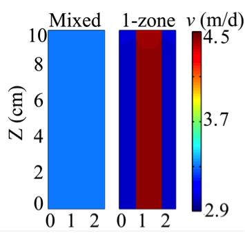 Figure 6: Flow fields of the Mixed and One-zone columns(figure from (Li et al., 2014))
In the homogeneous case, the flow velocity is 3.6 m/day for all the locations. For the One-zone column, the flow velocity in the magnesite zone is 4.5 m/day while the flow velocity in the sand zone is 2.9 m/day. The ratio of flow velocity between the magnesite zone and sand zone is 1.6, which is constant with the permeability ratio of the two zones.
-
For the 2D homogeneous domain, results should be similar to the 1D example in the lesson Flow and Transport Processes in 1D system except there is an additional parameter transverse dispersivity aT, a quantitative measure of dispersion in the direction transverse to the flow. Note that the aT value should not change the shapes of breakthrough curve as a function of residence time in the 2D homogeneous case because there is no transport limitation in the direction transverse to the main flow. Readers can analyze the sensitivity of differential pressure, dispersivity, molecular diffusion coefficient, and cementation factor.
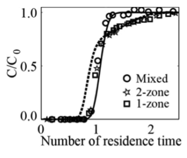 Figure 7. Breakthrough curves of the two columns (figure from (Li et al., 2014)).
8.5 Homework Assignment
In Heidari and Li (2014), 2D flow experiments and modeling were used to understand non-reactive solute transport in heterogeneous porous media with different spatial patterns. There are three two-dimensional (2D) sandboxes (21.9 cm × 20.6 cm) packed with the same 20% (v/v) fine and 80% (v/v) coarse sands in three patterns that differ in correlation length: Mixed, Four-zone, and One-zone. The Mixed cases contain uniformly distributed fine and coarse grains. The Four-zone and One-zone cases have four and one square fine zones, respectively (Figure 8).
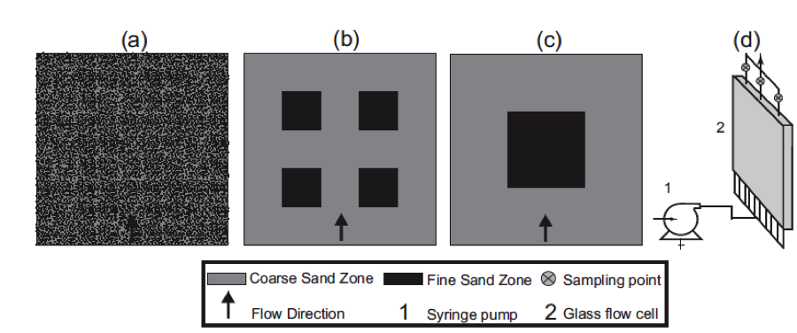
Read the paper carefully and follow the example in this lesson to generate the 2D flow fields and tracer breakthrough curves for the three sandboxes of high permeability contrast (HC). All parameters and properties of the three flow cells are in Table 1 and Table 2 in the paper. You can compare your modeling output of the flow field and breakthrough curves with Figure 5 (Flow field and local breakthrough curves) and Figure 6 (overall breakthrough curves from 2D model) in the paper. Note that one pore volume is the same as one residence time.
Note:
Apologies for no original CrunchFlow files for this hw. you can follow Example 8.1 and similarly set it up for this homework.
8.6 Summary and Final Tasks
Summary
In this lesson we studied general concepts and geostatistical measures of spatial heterogeneities, as well as how to set them up in 2D domains.
Reminder - Complete all of the Lesson 8 tasks!
You have reached the end of Lesson 8! Please make sure you have completed all of the lesson activities before you begin Lesson 7.
References
Boulanger, R. and Duncan, J. (2000) Geotechnical Engineering Photo Album: University of California at Davis, accessed March 15, 2006.
Bruderer-Weng, C., Cowie, P., Bernabé, Y. and Main, I. (2004) Relating flow channelling to tracer dispersion in heterogeneous networks. Adv. Water Resour. 27, 843-855.
Chen, C., Balhoff, M.T. and Mohanty, K.K. (2014) Effect of Reservoir Heterogeneity on Primary Recovery and CO2 Huff'n'Puff Recovery in Shale-Oil Reservoirs. SPE Reservoir Evaluation & Engineering.
Deutsch, C.V. and Journel, A.G. (1992) Geostatistical software library and user’s guide. New York.
Feehley, C.E., Zheng, C. and Molz, F.J. (2000) A dual‐domain mass transfer approach for modeling solute transport in heterogeneous aquifers: Application to the Macrodispersion Experiment (MADE) site. Water Resour Res 36, 2501-2515.
Fogg, G.E. (1986) Groundwater Flow and Sand Body Interconnectedness in a Thick, Multiple‐Aquifer System. Water Resour Res 22, 679-694.
Gelhar, L.W. (1986) Stochastic subsurface hydrology from theory to applications. Water Resour Res 22, 135S-145S.
Gelhar, L.W., Welty, C. and Rehfeldt, K.R. (1992) A critical review of data on field‐scale dispersion in aquifers. Water Resour Res 28, 1955-1974.
Harvey, C. and Gorelick, S.M. (2000) Rate‐limited mass transfer or macrodispersion: Which dominates plume evolution at the macrodispersion experiment (MADE) site? Water Resour Res 36, 637-650.
Heidari, P. and Li, L. (2014) Solute transport in low‐heterogeneity sandboxes: The role of correlation length and permeability variance. Water Resour Res 50, 8240-8264.
Hewett, T. (1986) Fractal distributions of reservoir heterogeneity and their influence on fluid transport, SPE Annual Technical Conference and Exhibition. Society of Petroleum Engineers.
Knudby, C. and Carrera, J. (2005) On the relationship between indicators of geostatistical, flow and transport connectivity. Adv Water Resour 28, 405-421.
Knudby, C. and Carrera, J. (2006) On the use of apparent hydraulic diffusivity as an indicator of connectivity. J Hydrol 329, 377-389.
Koltermann, C.E. and Gorelick, S.M. (1996) Heterogeneity in sedimentary deposits: A review of structure-imitating, process-imitating, and descriptive approaches. Water Resour Res 32, 2617-2658.
LaBolle, E.M. and Fogg, G.E. (2002) Role of molecular diffusion in contaminant migration and recovery in an alluvial aquifer system, Dispersion in Heterogeneous Geological Formations. Springer, pp. 155-179.
Li, L., Gawande, N., Kowalsky, M.B., Steefel, C.I. and Hubbard, S.S. (2011) Physicochemical heterogeneity controls on uranium bioreduction rates at the field scale. Environ Sci Technol 45, 9959-9966.
Li, L., Salehikhoo, F., Brantley, S.L. and Heidari, P. (2014) Spatial zonation limits magnesite dissolution in porous media. Geochimica Et Cosmochimica Acta 126, 555-573.
Li, L., Steefel, C., Kowalsky, M., Englert, A. and Hubbard, S. (2010) Effects of physical and geochemical heterogeneities on mineral transformation and biomass accumulation during a biostimulation experiment at Rifle, Colorado. J Contamin Hydrol 112, 45 - 63.
Mackay, D.M., Freyberg, D., Roberts, P. and Cherry, J. (1986) A natural gradient experiment on solute transport in a sand aquifer: 1. Approach and overview of plume movement. Water Resour Res 22, 2017-2029.
Murphy, E.M., Ginn, T.R., Chilakapati, A., Resch, C.T., Phillips, J.L., Wietsma, T.W. and Spadoni, C.M. (1997) The influence of physical heterogeneity on microbial degradation and distribution in porous media. Water Resour Res 33, 1087-1103.
Olsson, Å. and Grathwohl, P. (2007) Transverse dispersion of non-reactive tracers in porous media: a new nonlinear relationship to predict dispersion coefficients. J Contam Hydrol 92, 149-161.
Remy, N., Alexandre Boucher, and Wu., J. (2009) Applied Geostatistics with SGeMS. Cambridge University Press.
Renard, P. and Allard, D. (2013) Connectivity metrics for subsurface flow and transport. Adv Water Resour 51, 168-196.
Salamon, P., Fernàndez‐Garcia, D. and Gómez‐Hernández, J. (2007) Modeling tracer transport at the MADE site: the importance of heterogeneity. Water Resour Res 43.
Siirila-Woodburn, E.R. and Maxwell, R.M. (2014) A heterogeneity model comparison of highly resolved statistically anisotropic aquifers. Adv Water Resour.
Song, X., Hong, E. and Seagren, E.A. (2014) Laboratory-scale in situ bioremediation in heterogeneous porous media: Biokinetics-limited scenario. J Contam Hydrol 158, 78-92.
Sudicky, E.A. (1986) A natural gradient experiment on solute transport in a sand aquifer: Spatial variability of hydraulic conductivity and its role in the dispersion process. Water Resour Res 22, 2069-2082.
Willmann, M., Carrera, J. and Sánchez‐Vila, X. (2008) Transport upscaling in heterogeneous aquifers: What physical parameters control memory functions? Water Resour Res 44.
Zheng, C., Bianchi, M. and Gorelick, S.M. (2011) Lessons Learned from 25 Years of Research at the MADE Site. Ground Water 49, 649-662.
Zheng, C.M. and Gorelick, S.M. (2003) Analysis of solute transport in flow fields influenced by preferential flowpaths at the decimeter scale. Ground Water 41, 142-155.
Zinn, B. and Harvey, C.F. (2003) When good statistical models of aquifer heterogeneity go bad: A comparison of flow, dispersion, and mass transfer in connected and multivariate Gaussian hydraulic conductivity fields. Water Resour Res 39.
Lesson 9: Mineral Reactions in One-Dimension Systems
Overview
In this lesson we use a mineral reaction example to illustrate 1) how physical processes and geochemical processes are coupled in the short and long time scales, and 2) how to set up physical and geochemical processes in a 1D column in Crunchflow. The set up combines mineral dissolution (and precipitation) and physical flow processes in previous lessons. Please review these two lessons if needed.
Learning Outcomes
By the end of this lesson, you should be able to:
- Understand the importance of mineral dissolution and chemical weathering;
- Understand the fundamental principles and key parameters that govern chemical weathering and reactive transport process coupling in general;
- Set up simulations in CrunchFlow with flow, solute transport, and mineral dissolution and precipitation reaction.
Lesson Roadmap
| References (optional) | Review reading materials and examples on transport in 1D and mineral dissolution and precipitation |
|---|---|
| To Do |
|
9.1 Overview
Mineral dissolution and precipitation occur ubiquitously in natural systems. As minerals dissolve, chemicals in rocks are released into water, reducing solid mass and increasing aqueous concentrations. Mineral dissolution also opens up porosity for water storage. The opposite occurs when mineral precipitates and clog pore spaces. In the deep subsurface where we extract energy (e.g., oil, gas, geothermal energy) from, mineral dissolution and precipitation change the geochemical surface and water-conducting capacity, therefore regulating the energy extraction processes. Over geological times, the chemical and physical property alteration transforms rocks into soils and is called chemical weathering. Chemical weathering, together with physical weathering (erosion), shapes the Earth’s surface. Chemical weathering consumes carbon dioxide and locks them into carbonate minerals, which regulates the atmospheric CO2 level and sustain relatively clement earth conditions (Kump et al., 2000).
9.2 An example of mineral reactions in a 1D column
Example 9.1
A bedrock column is 10.0 meter deep with a porosity of 0.20. Mineral composition is simple with 80% v/v of quartz and 20% v/v of K-Feldspar. As the rainwater infiltrates through the rock, these primary minerals dissolve whereas a secondary mineral kaolinite precipitates, as listed in Table 1.
Conditions
The annual net runoff (precipitation – evapotranspiration) is 0.5 meter/year. Although we know that not all runoff infiltrates through the bedrock, for simplification here we assume the runoff flows through the bedrock and exits from the bottom of the bedrock. Assume the diffusion coefficients of all species are 1.0E-10 m2/s, and dispersivity is 0.1 m. The cementation factors are the default values of 1.0.
Let’s assume the initial pore water composition (all concentrations in molal): pH 7.0, Cl- (charge balance), K+ (4.0E-5), Na+ (4.0E-5), Al3+ (4.0E-6), HCO3- (1.0E-5), and SiO2(aq) (8.0E-5). One of the major drivers of chemical weathering is acidity. The acidity in soils comes primarily from the soil CO2 gas from root respiration and organic acids from root exudates. Here we set the total HCO3- concentration (equivalent to total inorganic carbon (TIC)) in the rainwater to 0.3 mM, which is equilibrated to soil gas CO2 of 9000 ppmv.
Question:
Assume chemical weathering occurs for 0.1 million years. Please set up the simulation in Crunchflow. Plot the profiles of pH, Saturation index $(\mathrm{SI}=[\log10(\mathrm{IAP}/\mathrm{K_{eq}})])$, $\phi$ ( volume of mineral/ volume of total porous media) of minerals and $\tau$ values of K and Si (relative to Zr in this soil column, we will explain later) at t = 0, 5,000, 10,000, 20,000, 40,000, and 100,000 years. How does the chemical composition and physical properties (e.g., porosity, permeability) evolve over time?
Note:
Setting up this lesson will involve what you learned from the lesson on mineral dissolution and precipitation, and the lesson on 1D transport. If needed please revisit these two lessons.
| Primary mineral dissolution | log10Keq |
log10k (mol/m2/s) |
Specific surface Area (m2/g) |
|---|---|---|---|
|
$\mathrm{SiO}_{2(\mathrm{s})}\text{(quartz)}\ \leftrightarrow\mathrm{\ SiO}_2\text{ (aq) }$ |
-4.00 | -13.39 | 0.01 |
| $\begin{array}{l} \mathrm{K} \mathrm{AlSi}_{3} \mathrm{O}_{8} \text { (K-Feldspar) }+4 \mathrm{H}^{+} \leftrightarrow \\ \mathrm{Al}^{3+}+\mathrm{K}^{+}+2 \mathrm{H}_{2} \mathrm{O}+3 \mathrm{SiO}_{2}(\mathrm{aq}) \end{array}$ |
-0.28 |
-13.00 -9.80aH+0.5 -10.15aOH-0.54 |
0.01 |
| Secondary mineral precipitation | |||
| $\begin{array}{l} \mathrm{Al}_{2} \mathrm{Si}_{2} \mathrm{O}_{5}(\mathrm{OH})_{4} \text { (Kaolinite) }+6 \mathrm{H}^{+} \leftrightarrow \\ 2 \mathrm{Al}^{3+}+2 \mathrm{SiO}_{2} \text { (aq) }+5 \mathrm{H}_{2} \mathrm{O} \end{array}$ |
6.81 | -13.00 | 0.01 |
*: Thermodynamic and kinetic parameters from EQ3/6 database [Wolery, 1992]. The three different rate constant values indicate the rate constants for neutral, acidic and basic kinetic pathways, respectively.
9.3 Governing Equations
A general governing equation for the mass conservation of a chemical species for a primary species i is the following:
where $\phi$ is porosity, Ci is the concentration (mol/m3), Dh is the hydrodynamic dispersion (m2/s), v is the flow velocity (m/s), ri,tot is the summation of rates of multiple reactions that the species i is involved (mol/ m3/s), and Np is the total number of primary species. Here we notice that this equation is very similar to the advection-dispersion equation that we discussed in previous lessons except for two major differences. One is that it has an additional reaction term ri,tot to take into account sources and sinks coming from mineral dissolution and precipitation. The other difference is that this is written for the species i, which is one of the Np primary species. Note that if the species is K+, the ri,tot in Equation (3) will be the summation of the K-feldspar reaction rate rK-feldspar and Kaolinite reaction rate rKaolinite. This is because K+ is involved in both of the kinetic reactions, the K-feldspar and Kaolinite reactions (either dissolution or precipitation). The mineral reaction rate laws follow the Transition State Theory (TST):
Where kH2O, kH, and kOH are the reaction rate constants with values of 10-13.0 mol/m2/s, 10-9.80 mol/m2/s under acidic conditions, and is the reaction rate constant of 10-10.15 mol/m2/s under alkaline conditions as shown, respectively (Table 1). The exponents of the H+ and OH- activities indicate the extent of rate dependence on H+ and OH-. A is the reactive mineral surface area (m2/m3 porous media). For kaolinite we have
Where kH2O is the reaction rate constant of 10-13.0 mol/m2/s as shown in Table 1.
In the chemical weathering context, K-feldspar dissolves and releases Al3+, K+, SiO2(aq), whereas Kaolinite precipitates and is the sink for Al3+ and SiO2(aq). The rate term in the parenthesis (1-IAP/Keq) is positive when minerals dissolve and is negative when minerals precipitate so we don’t need to change the sign of the rate term in the equation.
Species. The chemical species from the minerals are Al3+, K+, SiO2(aq). The species from the rainwater include H+, OH-, CO2(aq), HCO3-, CO32-, Na+, and Cl-. Here the major anions are the carbonate species so we can assume the aqueous complexes are KHCO3 (aq) and KCl (aq) and we have a total of 12 species. We can pick Al3+, K+, SiO2(aq), H+, HCO3-, Na+, and Cl- as primary species (7). This means we have secondary species including KHCO3(aq), KCl(aq), OH-, HCO3-, and CO32-. We need to solve for 12 (total number of all species) – 5 (total number of secondary species) = 7 primary species (governing equations).
9.4 At the short time scale: steady-state conditions
As the rainfall contacts the rock, cations and anions are released from the rock. The processes change properties of both solid and aqueous phases. However, the solid rock is dense in terms of amount of chemical mass compared to the aqueous phase so that the solid phase properties change at rates that are orders of magnitude slower than the aqueous phase. The system therefore often reaches steady state where the concentrations of species relatively constant over time.
The relative magnitude of advection, diffusion/dispersion and mineral dissolution are often compared using dimensionless numbers. The dimensionless numbers are quantitative measures of the relative magnitude of the characteristic time scales of different processes. In this case we have three characteristic time scales: the residence time related to advection $\tau\ \text{advection}=\frac{l}{v}$, the time for diffusion/dispersion $\tau\ \text {diffusion/dispersion}=\frac{l^{2}}{D_{h}}$, and the reaction time to reach equilibrium $\tau\ \text {reaction }=\frac{C_{e q}}{k A}$. Here we introduce two dimensionless numbers comparing the different time scales: DaI (Damköhler number for advection), DaII (Damköhler number for dispersion):
where l is the characteristics length of a domain (m), k is the rate constant (moles m−2 s−1), A is the reactive surface area (m2m−3), Dh is the diffusion coefficient in porous media (m2 s−1), and Ceq is the mineral solubility (moles m−3). When Damköhler number >>1, reaction times are much faster than transport times so that the system is transport controlled. The relative importance of advective versus dispersive transport is compared by the Péclet number that we have introduced before.
when Pe>>1, advective transport dominates and dispersive and diffusive transport are negligible.
9.5 At the long time scale: chemical weathering
If you have paid attention to a roadside cut, you will notice that the color, texture or structure along the direction of flow varies. This is because rocks at different depth have been subject to different extent of chemical weathering, resulting in gradients in mineral composition, reaction tendency, and porosity. Soils are generated over thousands to millions of years of chemical and physical alteration of their parent bedrock, which typically have much lower porosity and permeability than soils. Why and how are soils at different depth weathered differently? How do different parameters control chemical weathering?
Chemical and Physical Property Evolution
Mineral volume fraction
Using mass conservation principle, the code calculates the change in mass and volume in each mineral phase, which updates individual mineral volume fractions using the following equation:
Where $\phi_{j m, t}$ is the volume fraction of each mineral phase jm, Vjm is the molar volume of mineral jm, $r_{j m, t+\Delta t}$ is the the reaction rate of the mineral jm at time $t+\Delta t$. This can be done for each grid block in the domain.
Porosity
The porosity at any time $t$ can be updated as follows:
Where $\phi_t$ is the porosity at time $t$ and mtot is the number of solid phases.
Reactive surface area
The reactive surface area for mineral jm at time $t$, $A_{j m, t}$ is calculated based on the change in porosity and mineral volume fraction compared to their values at initial time 0 (Steefel et al., 2015):
Permeability
The local permeability in individual grid blocks is calculated using local porosity values from equation and the Kozeny-Carman equation (Steefel et al,. 2015):
Where $K_{t+\Delta t}$ is the permeability at time $t+D t$updated from time $. With updated permeability, flow velocities can be updated using Darcy's law. In this example, however, we use constant flow velocity for simplicity.
Quantification of chemical weathering: mass transfer coefficient $\tau$
Within a soil profile, $\tau$ is used to assess the effect of the chemical and physical alteration. Note that this is different from the time scale $\tau$ that we used previously on dimensionless numbers. We have to stick to this notation because the chemical weathering community uses $\tau$ for mass transfer coefficient, which is calculated by:
where $\tau_{i, j}$ is the mass transfer coefficient of element j relative to reference element i. cj,w and cj,p are the concentration of element j in weathered soil and in parent rock, respectively. ci,w and ci,p are the concentration of element i in weathered soil and in parent rock, respectively. The element i is considered as an immobile reference element to exclude the effects of the physical forces such as expansion/compaction. Titanium and zirconium are usually considered as immobile elements in calculating mass transfer coefficient. A negative $\tau_{i, j}$ value indicates mass loss while a positive $\tau_{i, j}$ value indicates mass enrichment for element j relative to element i. When $\tau_{i,j}=-1$, element j has been completely depleted as a result of the chemical weathering process. In calculating $\tau$ of K and Si relative to Zr, it is typically assumed that the soil column always has a constant concentration of immobile reference element Zr, which means $\frac{c_{Z r, p}}{c_{Z r, w}}=1$ all the time.
9.6 Example 9.1
Question
Assume the chemical weathering occurred for 0.1 million years. Please set up the simulation in Crunchflow. Plot the profiles of pH, Saturation index (SI, equal to [log10(IAP/Keq)]), $\phi$ ( volume of mineral/ volume of total porous media) of minerals and $\tau$ of K and Si relative to Zr in this soil column at the initial time, 5 thousand years, 10 thousand years, 20 thousand years, 40 thousand years and 100 thousand years. In calculating $\tau$ of K and Si relative to Zr, please assume the soil column always has a constant concentration of immobile reference element Zr, which means $\mathrm{C}_{\mathrm{Zr}, \mathrm{p}} / \mathrm{c}_{\mathrm{Zr}, \mathrm{w}}=1$ all the time. Discuss what you observe.
Note:
Setting up this lesson will involve what you learned from the lesson on mineral dissolution and precipitation, as well as the lesson on 1D transport. If needed please revisit these two lessons. In this lesson we do not provide videos and template anymore.
Please watch the following video: Mineral Dissolution and Precipitation 1D Columns (20:09)
Click here for CrunchFlow files [44]
Click for a transcript of the mineral dissolution and precipitation 1D Columns video
Mineral Dissolution and Precipitation 1D Columns
Li Li: OK, so this lesson we're going to talk about mineral dissolution, precipitation in one dimension, like, 1D columns. So this is different from the previous lessons that we had before on mineral dissolution and precipitation, which was in batch reactor, well-mixed systems. So it is really no dimension. Or you can call it a zero dimension because, in every spatial point, they are the same. So here, we are talking about 1D. What that means is that, essentially, you have a column. So we're talking about processes like, for example, rainfall comes in, hitting parent rock, and things dissolving out. And then, over a long period of time, these chemical species release out. And rock becomes soil.
So I'm going to use this as one example to talk about mineral dissolution and precipitation in 1D columns and how we set up these equations. But it's not really only about chemical weathering. It's really about these mineral dissolution precipitation reactions in general. In the short-terms, these reactions actually change, for example, water chemistry. If you think about a ground-water system, it would actually tend to-- we can see the change if there is mineral dissolution precipitation -- happen pretty fast. But in order to see change in the solid phase, we do need to wait a bit longer for enough change to happen. So today, I'm going to use this system. So I'll talk about this. If we're talking about rock transformation to become soil, we are setting up a system that has rainfall come in at a rate, maybe, for example, some way that is about annual precipitation minus e-t, something like that, at this flow velocity. And first thing, usually, we would have an unsaturated system in these topsoils, but for simplicity, we would just think about everything at the fully saturated system.
So it's easy at the beginning. So we have these systems that have essentially two minerals as parent rock. One is quartz -- and dissolves pretty slowly. Everyone knows about that. The other is K-feldspar, which is a very common silicate in rocks. K-feldspar has a formula of KAlSi and then O3-8. So essentially, you can think about this system-- if you think about rainfall, it comes in, dissolving out, and then releases these chemical species, that you can think about several processes as happening at the same time. One is advection. So this is the same advection we talked about in one unit set with a chaser, essentially, as the flow brings out the chemicals, but also there's a dispersion, diffusion. This again, is the same as what we talked about last time in the AD equations. But then the last one that is different from the previous, one other reaction, which is mineral dissolution precipitation reaction. So essentially this is like combining the AD equation unit with the mineral dissolution precipitation reaction unit. So if you need to go back, you're welcome to review this material. But essentially, because these three different processes are happening at the same time-- but then we also have multiple minerals -- we know the qualities are pretty slowly. And we can more or less think about this as almost non-reactive. Because compared to K-feldspar, it's a relatively very slow reaction. And when we think about the reaction that's happening, the K-feldspar will be dissolving out. So you would have this K-feldspar dissolving out to become released calcium, which is very important nutrients, metals, cations. And then it would be also released aluminum plus SiO2, so that's aqueous. These are species that are going to be coming out.
But at the same time, you also think about, some of these chemical species, when they reach a certain level, actually they can precipitate out as solid phase again. For example, aluminum plus SOi2 actually will become another mirror, which we call kaolinite. So essentially it will have the formula of Ai-Al2-Si2-O5-OH4. This is kaolinite. This is one type of very common clay in our system. Or if you go digging some soil, you will very easily see this type of clay. So essentially, you can think about the whole process as, like, you have parent bedrock. Rainfall comes in, releases some of the chemical species. But then some of these species also re-precipitate out. So it's almost like a redistribution of minerals. But at the same time, because some of species dissolving out over a long period of time, it would change the properties of the system, for example, porosity, permeability. Make this solid phase more permeable and have more pore space for water to flow through. So there's a change in physical properties as well.
So one question we often ask is how does this water and rock change over time and also over space? We want to know how fast things change and how much they change and what they have become. And a lot of time, we want to be able to predict that. So in order to do that, we have to come set up the equations, reactions, and all of that, putting everything together, and think about how we solve them.
So again, with the system, every time we need to think about the chemical system and how they evolve over time and space, we think-- the first thing we need to think about-- the chemical species first. So you have several primary species again. If you review back some of the material we covered before, we had primary species, then existent system-- because we have aluminum, silica-- that they have to be there. This has to be part of the building block of the system. You have potassium too. And when the rainfall comes in, usually it brings some acidity. So H-plus should be there. You would also have CO2-aq. In addition, a lot of times, these rainfalls have a little bit of salt in them. So to be representative, we are also putting a bit of sodium chloride in that example-- sodium chloride as part of the rainfall. That means, also, in the second species, we need to decide, OK, what complexities would be formed, how much can complex reaction happen, and things like this. So to keep it simple, I'm going to just have potassium and then HCO3-aq and maybe KCl-aq as two complexities. And then, of course, we also need other species, for example, H-minus. We need the other form of bicarbonate and carbonate. So it's quickly become a long list of species.
So if we are talking these chemical species, we'll be essentially solving for 1, 2, 3, 4, 5, 6, 7. We'll have seven primary species. So that essentially means we would have seven independent equations to solve for. So what I'm writing here is a general type of governing equation, for one species, I. And again, this first term-- we call, mass accumulation term, that we discussed before. Is a summation of overall change. And then you have the advection term, diffusion term, dispersion term. These doesn't change, because of the system. But for example, the primary would change, but the terms wouldn't change. You could have different porosity phi or velocity or diffusion-dispersion coefficient for a different chemical species. But the term itself wouldn't change. And then the last term is new. It's a reaction term. So it would take into account, essentially, different types or the rates of different types of reactions that this species, I, is involved in. And you think about how fast these different reactions would change in the continuation of species I. And of course, this I needs to be written for 1 to Np, which is the number of primary species. So you need to write, for this system, seven different equations to solve. But then, on top of that, again, you have this number of secondary species you need to solve for in the form of algebraic relationships.
So how does this r-i-j look? These are terms different from the previous AD equations, that without this term. Now here, this r is a [INAUDIBLE] term. So you have that. So for this, r's, it needs to be-- everything about this particular r-- let's make this i is potassium. So for potassium, means this system-- you can think about two reactions involved in. One is that the K-feldspar dissolving out to release out calcium. And then it comes out. And it goes. So actually, one reaction-- so it would be just K-feldspar dissolving out. So if it's K, then you would just have this rate. And then you follow TST rate all right. So you have, probably, this complicated K-H-plus, dependence on H-plus, whatever term, empirical numbers, K-H2O and then a water plus KOH-minus and then Activity OH-minus-- some empirical exponent here as well. These are the regular part, early part, that depends on pH. But then, again, you have surface area. And the last term would be 1 minus IAP over K-aq. Again, it's how fast this is close to equilibrium or far away from equilibrium. So that's the general form of reaction rate law. So when we solve equals to this term, we'll be putting there-- so this is going to be a complicated term. But also, if you think about, for example, species like aluminum or silica, then they're actually involving two different reactions. One is K-feldspar dissolving out to release these. But a kaolinite also precipitated out. So there's one source reaction term and r-i term. And the other would be a sink term for kaolinite precipitating out. So it's a sink for aluminum or silica.
So we solve all of these equations. And what we come up with is all these Ci as a function of time and space. So you have X versus-- essentially, once we know all the parameters, initial conditions, bounded conditions-- what water comes in, what water comes out the beginning, what's the pore water composition in the rock and all that, this will give us this distribution of concentration from time and space. And over geological time, when this changes line-- and when I say geological time, I mean at least thousands of years, thousands or 10 thousands or close to 1 million years, things like that. So over this time scale, you would have these things keep on changing. And then the rock becomes soil, property of the porous media change. You have porosity increases typically. And you have, also, permeability change, because the water-- the resistance of this porous media to water becomes lower and lower. So you have permeability increase as well. So this would be the chemical weathering over long-term. Over short-term, is all of these reaction changes or water chemistry.
But the last part of it, I want to mention a little bit about the dimensionless number, from the mass point-of-view, how these would change, how we analyze these systems. So last time, when we talked about this equation of AD with other reaction term, we talked about the Pe or Peclet number, which is the tau of the advection. It's a tau diffusion-dispersion over tau advection. Tau is a time scale, right? So the time scale of diffusion and dispersion, which is L squared over D-- so it's length of this column-- over diffusion-- because that's the time scale for diffusion-dispersion-- divided by-- or times, if I do it this way-- times 1 over tau-a, which is the opposite of lance over advection. So you would have v-L. So that cancels out. It becomes L-v over D. And so that's a Peclet number, that we talked of before. So this term essentially compares the relative magnitude of advection versus diffusion-dispersion. Which point is dominant under phosphoro or slow conditions? But then, because we have the reaction term, we have two more different dimensionless numbers, we call Damkohler numbers. So the first step-- because think about, we have two transport processes. One is diffusion-dispersion. Other is the advection. So the first one is comparing the time scale of reaction-- the relative time scale of advection to the relative time scale of reaction. And in that case, again, tau-a would be the same as L over v. But then, you'd be-- this is over tau reaction. For reaction, we are thinking about how much things can dissolve and, eventually, reach equilibrium. So you would have total bulk volume times porosity, which is how much pore space you have that can hold water. So that's a lot of volume times the maximum concentrations and you can dissolving out, divided by the rate constant as a maximum, K times A. So this would be, essentially, the reaction time, the characteristic time for reaction. And in notes, I have simplified this. And you can have that. You can look at these. For the second Damkohler number, you would be comparing the time scale of diffusion-dispersion over tau-r. And again, this would be going back to L squared over D, divided by the same thing. Because the reserve reaction term would be the same.
So if you think about-- we typically talk about, under fast reaction system, fast compared to transfer versus when you have very slow reaction systems. So when you have very fast reaction systems, the systems tend to reach equilibrium quickly. And we tend to be transporter-controlled. It would be determined by the bottleneck of all processes, which mean it's going to be transport-controlled. If the reaction is actually slower-- so you will see, by this analysis, you will be able to tell how the system would behave, whether it's transport-controlled or surface reaction-controlled. And how these will be changing over distance and time will give us some kind of grouping analysis that we can do.
So I'm going to end here. I'm going to go back and look at notes. And this, I went through pretty fast. So look at notes we have. Do some homework. And you will realize, these analyses will really help you to understand how things are different under different conditions.
Click for Solution
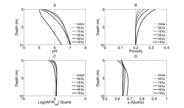
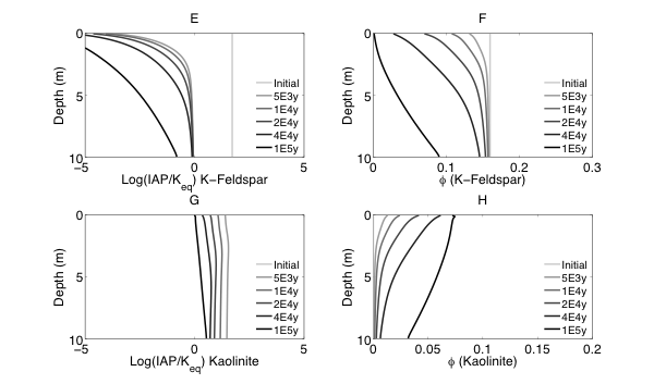
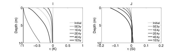
Figure 2 Evolutions of (A) pH (B) porosity (C) Saturation Index $\left[\log 10\left(I A P / K_{e q}\right)\right]$ of K-Quartz, (D) $\phi$(Quartz) (volume of Quartz / volume of total porous media) (E) Saturation Index $\left[\log 10\left(I A P / K_{e q}\right)\right]$ of K-Feldspar (F) $\phi$ (K-Feldspar) (volume of K-Feldspar / volume of total porous media) (G) Saturation Index $\left[\log 10\left(I A P / K_{e q}\right)\right]$ of Kaolinite, (H) $\phi$(Kaolinite) (volume of Kaolinite / volume of total porous media), $\text { (I) } \tau(K)$ and $\text { (J) } \tau(S i)$ as a function of soil depth at different times.
Initially, the pH in the rock is 6 and porosity is 0.2. After the simulation starts, rainwater flows into the soil column from the top with a lower pH so the pH in the upper column (close to the surface) decreased. In the lower part of the column, incoming hydrogen ion is consumed during mineral dissolution so pH increases. As mineral dissolves, porosity is enlarged. Porosity increases more where mineral dissolution is faster. Because rainwater has lower pH and lower solute concentrations, Quartz is under saturated and dissolves from the top. However, because the lower part of column has a higher pH, Quartz is re-precipitating in the lower part of column. K-Feldspar is under saturated throughout the column so it always dissolves. Kaolinite precipitates as a secondary mineral as K-Feldspar and quartz dissolve and elevate the aqueous concentrations.
From the discussion above it is apparent that soil at different depth weathers differently primarily due to the availability of reactants for the dissolution reactions at different depth. The delivery through flow and transport and the consumption of reactants compete with each other in the soil profile, which determines the location and shape of the weathering front. In fact, the extent and speed of chemical weathering can often be interpreted inversely based on understandings of the vertical profile through numerical simulations [Brantley and White, 2009].
9.7 Homework Assignment
Please pick one of the following for homework assignments.
1) Chemical Weathering (Example 9.1 extension, total 60 points, 15 points each):
assess the role of dissolution rates, dissolution kinetics, rainwater chemistry, and rainwater abundance.
Continuing along example 1, please analyze the role of different parameters/conditions in determining chemical weathering rates and profile. In each of the questions below, please compare the base case in the example to two more cases with different parameter values. In each question, please keep all other parameters and conditions the same so we can fully focus on the effects of the changing parameter. In each question, draw the depth profiles of porosity, volume fractions of Quartz, K-Feldspar, and Kaolinite, and $\tau$ figures at 100,000 years:
- 1.1) Effects of K-Feldspar dissolution rates: K-Feldspar rate 10 and 100 times slower;
- 1.2) Effects of K-Feldspar equilibrium constants: 1 order of magnitude larger or 1 order of magnitude smaller;
- 1.3) Effects of rainwater composition: change the total inorganic carbon (HCO3-) concentration by 2 times larger or 2 times lower, to represent changing CO2 content in rainwater;
- 1.4) Effects of annual rainfall (flow velocity): increase and decrease by 2 times.
Click here for CrunchFlow Solutions. [45]
2) Calcite dissolution in a 1D homogeneous column (short time scale, total 60 points).
In a homogeneous column at the length of 10.0 cm and diameter of 2.5 cm, calcite and sand grains are uniformly distributed in the column. Detailed physical and geochemical properties are in Table 2.
| Parameters | Values |
|---|---|
| Calcite (gram) | 14.62 |
| Quartz (gram) | 76.10 |
| Grain Size Calcite ($\mu m$) | 225-350 |
| Grain Size Quartz ($\mu m$) | 225-350 |
| BET SSA of Calcite (m2/g) | 0.115 |
| BET SSA of Quartz (m2/g) | 0.41 |
| AT Calcite (m2) | 1.68 |
| $\phi \text { ave }$ | 0.40 |
| $k_{e f f}\left(x 10^{-13} m^{2}\right)$ | 8.20 |
| Local longitudinal dispersivity $a_{L}(\mathrm{~cm})$ | 0.20 |
The initial and inlet solution conditions are listed in Table 3. Flushing through experiments were carried out at flow velocities of 0.1, 0.3, 3.6, 7.2 and 18.5 m/d at pH 4.0. Prior to dissolution experiments, each of the columns was flushed with 10-3 mol/L NaCl solution at pH 8.8 at 18.0 m/d to flush out pre-dissolved Ca(II) for a relatively similar starting point.
| Species | Initial Concentrations (mol/L, except pH) | Inlet Concentrations (mol/L, except pH) |
|---|---|---|
| pH | 8.8 | 4.0 for all columns and 6.7 only for Kratio,Ca/Qtz at 0.5 (in dissolution experiment) 8.8 (in tracer experiment) |
| Total Inorganic Carbon (TIC) | 1.0x10⁻³ (Approximate, close to equilibrium with calcite) | 1.0x10⁻¹⁰ to 1.0x10⁻⁵ (depending on experimental conditions, some contain CO2 bubbles) |
| Ca(II) | Varies between 1.0x10⁻⁵ to 1.5x10⁻⁴ depending on experimental conditions | 1.0x10⁻²⁰ |
| Na(I) | 1.0x10⁻³ | 1.1x10⁻³ |
| Cl(-I) | 1.0x10⁻³ | 1.0x10⁻³ |
| Br(-I) | 1.0x10⁻²⁰ | 1.2x10⁻⁴ |
| Number | Kinetic reactions | Log Keq | kCa (mol/m2/s) |
|---|---|---|---|
| (1) | $\mathrm{CaCO}_{3}(s)+\mathrm{H}^{+} \Leftrightarrow \mathrm{Ca}^{2+}+\mathrm{HCO}_{3}^{-}$ | 1.85 | 1.0x10⁻² |
| (2) | $\mathrm{CaCO}_{3}(s)+\mathrm{H}_{2} \mathrm{CO}_{3}^{0} \Leftrightarrow \mathrm{Ca}^{2+}+2 \mathrm{HCO}_{3}^{-}$ | -- | 5.60x10⁻⁶ |
| (3) | $\mathrm{CaCO}_{3}(s) \Leftrightarrow \mathrm{Ca}^{2+}+\mathrm{CO}_{3}^{2-}$ | -- | 7.24x10⁻⁹ |
Reaction (1) dominates when pH<6.0; reaction (3) dominates at higher pH conditions: reaction (2) are important under CO2- rich conditions.
Please do the following:
2.1) Calculate the pore volume (total volume of pore space), residence time $\tau_{a}$, and Peclet number (Pe) at each flow velocity;
2.2) Set up simulation for each flow velocity, and plot the breakthrough curves (BTCs, concentrations as a function of $\tau_{a}$) under each flow condition for Ca(II), IAP/Keq, and pH; plot one figure for each (Br, Ca(II), IAP/Keq, and pH) so you have all BTCs under different flow conditions in the same figure; comment on the role of flow in determining calcite dissolution and why; Here breakthrough curve is defined as concentrations vs time at the last grid block of the column.
2.3) Calculate the steady-state column-scale rates under each flow velocity by R = Q(Ceffluent – Cinfluent). Note that Q (volume/time) = u * Ac, where u is the Darcy flow velocity, Ac is the cross-sectional area of the column; Also note that "steady-state conditions" means the conditions under which concentrations in each grid do not change with time any more.
2.4) Calculate the DaI and DaII (again, under steady state) for each flow velocity;
2.5) Make a table of v, R, $\tau$, Pe, and Da numbers at each flow velocity. Plot R as a function of Pe and DaI and DaII.
9.8 Summary
Summary
In this lesson, we introduced the basic principles of transport and mineral reaction coupling in the context of chemical weathering process and how soils are formed.
References
Brantley, S. L., and A. F. White (2009), Approaches to Modeling Weathered Regolith, Thermodynamics and Kinetics of Water-Rock Interaction, 70, 435-484.
Kump, L. R., Brantley, S.L. and Arthur, M. A. (2000), Chemical weathering, atmospheric CO2, and climate, Annual Review of Earth and Planet Science, 28, 611 - 667.
Steefel, C.I., Appelo, C.A.J., Arora, B., Jacques, D., Kalbacher, T., Kolditz, O., Lagneau, V., Lichtner, P.C., Mayer, K.U., Meeussen, J.C.L., Molins, S., Moulton, D., Shao, H., Šimůnek, J., Spycher, N., Yabusaki, S.B. and Yeh, G.T. (2015) Reactive transport codes for subsurface environmental simulation. Computational Geosciences 19, 445-478.
Wolery, T. J. (1992), EQ3/6: A software package for geochemical modeling of aqueous systems: Package overview and installation guide (version 7.0), Lawrence Livermore National Laboratory Livermore, CA.
Lesson 10: Mineral Dissolution in Two Dimensional Systems
Overview
In this lesson we will set up 2D reactive transport systems in both homogeneous and heterogeneous domains. You will learn 1) how physical and geochemical processes are coupled, and 2) how spatial heterogeneity controls reaction processes. In essence, this lesson combines 2D transport and mineral dissolution and precipitation lesson. Please review these two lessons if necessary.
Learning Outcomes
By the end of this lesson, you should be able to:
- Understand how mineral dissolution and transport are coupled;
- Set up simulations in Crunchflow with flow, solute transport, and mineral dissolution and precipitation reaction in 2D homogeneous and heterogeneous systems.
10.1. Introduction
In this lesson we are not going to introduce new concepts. The flow and transport processes in homogeneous and heterogeneous systems (1D and 2D) have been introduced before. Similarly, mineral dissolution has also been discussed in a previous lesson. These processes are typically coupled in heterogeneous porous media, meaning they can affect each other. That is, flow influences reactions, and reactions can also have impacts on flow.
In a system where both physical flow and transport and reactions coexist, a general governing equation for any dimension system is as follows:
where Φ is porosity, Ci is the concentration of a primary aqueous species i (mol/m3), D is the hydrodynamic dispersion tensor (m2/s), u is the flow velocity (m/s), ri,tot is the summation of rates of multiple reactions that the species i is involved (mol/ m3/s) , and Np is the total number of primary species. Solving Np equations simultaneously gives the concentrations of primary species at different time and locations, which can then be used to solve for the concentrations of secondary species through laws of mass action (equilibrium relationship of fast reactions).
The equation (1) is general for systems with different number of dimensions (one, two, or three dimensions). Note that this is similar to the governing equation that we discuss in the 1D chemical weathering lesson, except that here we do not specify the dimension. If we specify this for 1D system, it will then be the same from as the governing equation in the 1D chemical weathering lesson.
Also note that in this equation, the dispersion coefficient and the velocities are written as tensors or matrix (in bold symbols) and can have different values in different locations. In fact, all porous medium properties, including porosity, permeability, and surface area can have spatial variations, as we will see in the example.
10.2. Setting up magnesite dissolution in homogenous and heterogeneous columns
Here we will build upon example 8.1 in lesson 8 to illustrate a magnesite dissolution example in homogeneous and heterogeneous 2D systems based on the experiments in Li et al. (2014). I am reiterating the example 8.1 here.
Example 11.1
The following gives an example of setting up flow and transport calculations in 2D homogeneous and heterogeneous domains. Here we use the physical set up of 2D cross-sections of the Mixed and One-zone column in (Li, Salehikhoo et al. 2014). The authors packed 4 columns of 2.5 cm in diameter and 10.0 cm in length with relatively similar amount of magnesite and quartz distributed in different spatial patterns. Here we focus on two columns that represent two extreme cases: the Mixed column with uniform distributed magnesite and quartz, as well as the One-zone column with magnesite all clustered in one cylindrical zone of diameter of 1.0 centimeter. To keep it simple, here we will do the calculation for 2D cross-sections, instead of following the steps in section 3.2.4 in the paper to convert 2D to 3D. So our numbers might be different from the paper. We are also assuming that in the middle one zone magnesite is 100% of the solid phase and the Mixed column has the same total amount of magnesite as in the One-zone case. The 2D system has a size of 25 mm by 100 mm. A constant differential pressure is imposed at the boundaries in the z (vertical) direction, leading the primary water flow direction in the z direction from the bottom to the top. No flux boundaries are specified in the X direction (Li, Salehikhoo et al. 2014).
| Columns | Mg zone | Qtz zone | 2aL (cm) |
4aT (cm) |
ke (× 10-13m2) |
Φ avg |
|---|---|---|---|---|---|---|
| Mixed | - | - | 0.05 | 0.005 | 8.26 | 0.44 |
| One-zone | Width: 1.0 cm ΦMg: 0.54 |
Width: 1.5 cm ΦQtz: 0.38 |
0.07 | 0.004 | 10.74 | 0.44 |
*The permeability of the pure sand columns of the same grain size was measured to be 8.7×10⁻¹³ m2.
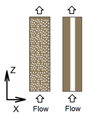
We have shown in the example and video how we calculate the flow field, solute transport, and breakthrough of these two columns. In this lesson we will add the reaction component of this experiment, which is magnesite dissolution. The reaction network and the inlet and boundary conditions are listed in Table 1 and Table 2, respectively. The experiment injected acidic water (inlet) into the two columns, dissolving magnesite. As you probably notice here, the only kinetically-controlled reactions are magnesite dissolution.
| Log Keq | k (mol/m2/s) | SSA (m2/g) BET, measured |
|
|---|---|---|---|
| Aqueous speciation (at equilibrium) | |||
| -14.00 | - | - | |
| -6.35 | - | - | |
| -10.33 | - | - | |
| -1.04 | - | - | |
| -2.98 | - | - | |
| Kinetic reactions (logK value is logKsp value) | |||
| - | 6.20×10⁻⁵ | 1.87 | |
| - | 5.25×10⁻⁶ | 1.87 | |
| -7.83 | 1.00×10⁻¹⁰ | 1.87 |
| Species | Initial Concentrations (mol/L, except pH) |
Inlet Concentrations (mol//L, except pH) |
|---|---|---|
| pH | 8.8 | 4.0 |
| Total Inorganic Carbon (TIC) | 3.43E-3 (Approximate, close to equilibrium with magnesite) | 1.07E-5 (in equilibrium with CO2 gas) |
| Mg(II) | Varies between 0.52E-5 to 1.20E-5, depending on experimental conditions | 0.0 |
| Na(I) | 1.00E-3 | 1.00E-3 (in dissolution experiment) 1.12E-3 (in tracer experiments) |
| Cl(-I) | 1.00E-3 | 1.00E-3 |
| Br(-I) | 0.0 | 0.0 (in dissolution experiments) 1.20E-4 (in tracer experiments) |
| Si(VI) | 1.00E-5 | 1.00E-4 |
* The measured quantities include pH, total aqueous Mg(II), Na(I), Cl(-I), Br(-I), and Si(VI). Concentrations of all individual species were calculated using the speciation calculation in CrunchFlow based on thermodynamic data in Eq3/6 (Wolery et al., 1990)
In this example, the species from the inlet water include H+, OH-, CO2(aq), HCO3-, CO32-, Na+, Cl-, and Mg2+. Here the major anion is carbonate species so we assume the major aqueous complexes areMgHCO3+ and MgCO3 (aq), as shown in Table 1. This means that we need to solve for 8 (total number of all species) – 5 (total number of secondary species) = 3 governing equations. Note that the ri,tot here should be the total magnesite dissolution rate through the three reaction pathways listed in Table 1:
Where all rate constants and surface area as shown in Table 1. Please note that in such columns, you can calculate the overall magnesite dissolution rates at the column scale using mass balance of the column:
Here RMgCO3 is the column-scale magnesite dissolution rates, CMg(II),out is the average Mg(II) concentration coming out of the column outlet, and CMg(II),in is the average Mg(II) concentration coming into of the column. Here please note that we use Mg(II) to represent the total concentrations of Mg(II), instead of individual species such as Mg2+ and MgHCO3+. , where CMg(II),i and qi are the concentration and flow rate from the grid block i in the outlet cross-section. With the same inlet solution across the inlet cross-section, you can directly use the inlet concentration for the calculation.
10.3. Homework assignment
Question
Given the above geochemical conditions above and the physical flow and transport given in lesson 8, please set up the 2D Mixed and One-zone magnesite dissolution columns. Please answer the following questions:
- Effects of flow rates:
- At the average flow velocity of 3.6 m/day, please
- compare the spatial profiles of Mg(II) in the two columns at the residence time of 3.0.
- draw the Mg(II) breakthrough curves using the equation for CMg(II),out,. Note that similar to the example in lesson 8, you will need to do this calculation for multiple time points. Which column dissolves magnesite faster under steady state conditions? By how much? Please show steps of calculation.
- At the average flow velocity of 0.36 m/day,please answer the same two questions as in question 1).
- At the average flow velocity of 36.0 m/day, please answer the same two questions as in question 1).
- Please summarize your observations from questions 1) to 3). What are the effects of flow velocities on the column-scale dissolution rates? Why are rate differences between the two columns similar under some flow conditions, and more different under other conditions?
- At the average flow velocity of 3.6 m/day, please
- (optional) Effects of transverse dispersivity aT: If you increase or decrease the transverse dispersivity aT, what difference does it make for the column-scale dissolution rates and spatial patterns of Mg(II) ? Do you think aT is important in controlling column-scale dissolution rates? If so, why?
10.4. Summary
In this lesson, we learned how to couple physical flow and transport with mineral dissolution in 2D systems with both homogeneous and heterogeneous spatial distribution of minerals. We can do this similarly for other types of reactions, including surface complexation, ion exchange, and microbe-mediated reactions. Flow has fundamental impacts on how fast reactions occur. In long time scales where the extent of reaction is sufficient to change porous medium properties, the reactions also affect the flow processes.
Reference
Li, L., F. Salehikhoo, S. L. Brantley and P. Heidari (2014). "Spatial zonation limits magnesite dissolution in porous media." Geochimica Et Cosmochimica Acta 126(0): 555-573.