Course Outline
Lesson 1: Retrieving Data From a Relational Database
Overview
Overview
One of the core skills required by database professionals is the ability to manipulate and retrieve data held in a database using Structured Query Language (SQL, sometimes pronounced "sequel"). As we'll see, queries can be written to create tables, add records to tables, update existing table records, and retrieve records meeting certain criteria. This last function, retrieving data through SELECT queries, is arguably the most important because of its utility in answering the questions that led the database developer to create the database in the first place. SELECT queries are also the most fun type to learn about, so, in this first lesson, we will focus on using them to retrieve data from an existing database. Later, we'll see how new databases can be designed, implemented, populated and updated using other types of queries.
Objectives
At the successful completion of this lesson, students should be able to:
- use the Query Builder GUI in MS-Access to create basic SQL SELECT queries;
- understand how settings made in the Query Builder translate to the various clauses in an SQL statement;
- use aggregation functions on grouped records to calculate counts, sums, and averages;
- construct a query based on another query (subquery).
Questions?
Conversation and comments in this course will take place within the course discussion forums. If you have any questions now or at any point during this week, please feel free to post them to the Lesson 1 Discussion Forum.
Checklist
Checklist
Lesson 1 is one week in length (see the Canvas Calendar for specific due dates). To finish this lesson, you must complete the activities listed below:
- Download the baseball stats.accdb [1] (right-click and Save As) Access database that will be referenced during the lesson.
- Work through Lesson 1.
- Complete Project 1 and upload its deliverables to the Project 1 Dropbox.
- Complete the Lesson 1 Quiz.
SELECT Query Basics
SELECT Query Basics
Why MS-Access?
A number of RDBMS vendors provide a GUI to aid their users in developing queries. These can be particularly helpful to novice users, as it enables them to learn the overarching concepts involved in query development without getting bogged down in syntax details. For this reason, we will start the course with Microsoft Access, which provides perhaps the most user-friendly interface.
A. Download an Access database and review its tables
Throughout this lesson, we'll use a database of baseball statistics to help demonstrate the basics of SELECT queries.
- Click to download the baseball database. [1]
- Open the database in MS-Access.
One part of the Access interface that you'll use frequently is the "Navigation Pane," which is situated on the left side of the application window. The top of the Navigation Pane is just beneath the "Ribbon" (the strip of controls that runs horizontally along the top of the window).
The Navigation Pane provides access to the objects stored in the database, such as tables, queries, forms, and reports. When you first open the baseball_stats.accdb database, the Navigation Pane should appear with the word Tables at the top, indicating that it is listing the tables stored in the database (PLAYERS, STATS, and TEAMS). - Double-click on a table's name in the Navigation Pane to open it. Open all three tables and review the content. Note that the STATS table contains an ID for each player rather than his name. The names associated with the IDs are stored in the PLAYERS table.
B. Write a simple SELECT query
With our first query, we'll retrieve data from selected fields in the STATS table.
- Click on the Create tab near the top of the application window.
- Next, click on the Query Design button (found on the left side of the Create Ribbon in the group of commands labeled as Queries).
When you do this in Access 2010 and higher, the ribbon switches to the Design ribbon. - In the Show Table dialog, double-click on the STATS table to add it to the query and click Close.
- Double-click on PLAYER_ID in the list of fields in the STATS table to add that field to the design grid below.
- Repeat this step to add the YEAR and RBI fields.

- At any time, you can view the SQL that's created by your GUI settings by accessing the View drop-down list on the far-left side of Design Ribbon (it is also available when you have the Home tab selected, as shown below).
As you go through the next steps, look at the SQL that corresponds to queries you are building.
C. Restrict the returned records to a desired subset
- From the same View drop-down list, select Design View to return to the query design GUI.
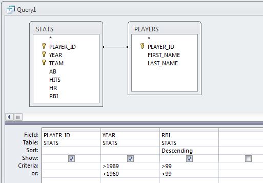
- In the design grid, set the Criteria value for the RBI field to >99.

- Test the query by clicking on the red exclamation point on the top left next to the View dropdown (it should return 103 records).
D. Sort the returned records
- Return to Design View by selecting it from the View dropdown.
- In the design grid, click in the Sort cell under the RBI column and select Descending from the drop-down list. This will sort the records from highest RBI total to lowest.
- Test the query.
E. Add additional criteria to the selection
- Return to Design View and set the Criteria value for the YEAR field to >1989. This will limit the results to seasons of over 100 RBI since 1990.
- Test the query (it should return 53 records).
- Return to Design View and modify the Criteria value for the YEAR field to >1989 And <2000, which will further limit the results to just the 1990s.
- Test the query (it should return 34 records).
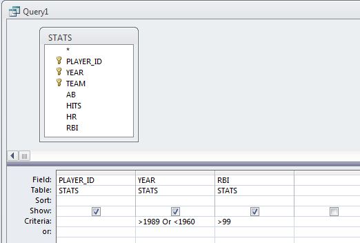
- Return to Design View and change the Criteria value for the YEAR field back to >1989, beneath that cell (in the or: cell) add <1960.
As you should be able to guess, I'm asking you to write a query that identifies 100-RBI seasons since 1989 OR prior to 1960. However, the query as written at this point doesn't quite yield that result; look at the WHERE line in the SQL view. Instead, it would return 100-RBI seasons since 1989 and all seasons prior to 1960 (not just the 100-RBI ones). To produce the desired result, you need to repeat the >99 criterion in the RBI field's or: cell. Check the SQL view to see the change.
- Test the query (it should return 74 records).
You've probably recognized by now that the output from these queries is not particularly human friendly. In the next part of the lesson, we'll see how to use a join between the two tables to add the names of the players to the query output.
Joining Data From Multiple Tables
Joining Data From Multiple Tables
One of the essential functions of an RDBMS is the ability to pull together data from multiple tables. In this section, we'll make a join between our PLAYERS and STATS tables to produce output in which the stats are matched up with the players who compiled them.
A. Retrieve data from multiple tables using a join
- Return to Design View and click on the Show Table button (near the middle of the Ribbon).
- In the Show Table dialog, double-click on the PLAYERS table to add it to the query, then Close the Show Table dialog. Create the join by click-holding on the PLAYER_ID field name in one of the tables and dragging to the PLAYER_ID field name in the other table. If you make the wrong join connection, you can right-click on the line and delete the join.
Note:
You'll probably notice the key symbol next to PLAYER_ID in the PLAYERS table and next to PLAYER_ID, YEAR and TEAM in the STATS table. This symbol indicates that the field is part of the table's primary key, a topic we'll discuss more later. For now, it's good to understand that a field need not be a key field to participate in a join, and that while the fields often share the same name (as is the case here), that is not required. What's important is that the fields contain matching values of compatible data types (e.g., a join between a numeric zip code field and a string zip code field will not work because of the mismatch between data types).
- Modify the query so that it again just selects 100-RBI seasons without any restrictions on the YEAR.
- Double-click on the FIRST_NAME and LAST_NAME fields to add them to the query.
- Test the query. Looking at the output, you may be thinking that the PLAYER_ID value is not really of much use anymore and that the names would be more intuitive on the left side rather than on the right.
- To remove the PLAYER_ID field from the output, return to Design View and click on the thin gray bar above the PLAYER_ID field in the design grid to highlight that field. Press the Delete key on your keyboard to remove that field from the design grid (and the query results).
- To move the name fields, click on the FIRST_NAME field's selection bar in the design grid and drag to the right so that you also select the LAST_NAME field. With both fields selected, click the selection bar and drag them to the left so that they now appear before the YEAR and RBI fields.

- Test the query.
B. Use the Expression Builder to concatenate values from multiple fields
- Return to Design View and right-click on the Field cell of the FIRST_NAME column; on the context menu that appears, click on Build to open the Expression Builder.
You should see the FIRST_NAME field listed in the expression box already. Note the Expression Elements box in the lower left of the dialog, which provides access to the Functions built into Access (e.g., the LCase function for turning a string into all lower-case characters), to the tables and fields in the baseball_stats.accdb database (e.g., STATS), to a list of Constants (e.g., True and False) and to a list of Operators (e.g., +, -, And, Or). All of these elements can be used to produce expressions in either the Field or Criteria rows of the design grid. Note that it's also OK to type the expression directly if you know the correct syntax. Here, we're going to create an expression that will concatenate the FIRST_NAME value with the LAST_NAME value in one column. - First, delete the FIRST_NAME text from the expression box.
- Expand the list of objects in the baseball_stats.accdb database by clicking on the plus sign to its left. Then expand the list of Tables.
- Click on PLAYERS to display its fields in the middle box. Double-click on the FIRST_NAME field to add it to the expression. (Note that the field is added to the expression in a special syntax that includes the name of its parent table. This is done in case there are other tables involved in the query that also have a FIRST_NAME field. If there were, this syntax would ensure that the correct FIRST_NAME field would be utilized.)
- The concatenation character in Access is the ampersand (&). Click in the expression text box after [PLAYERS]![FIRST_NAME] to get a cursor and type:
& ' ' &
So, you type &-space-single quote-space-single quote-space-&. The purpose of this step is to add a space between the FIRST_NAME and LAST_NAME values in the query results. - Double-click on the LAST_NAME field in the field list to add it to the expression.
- Finally, place the cursor at the beginning of the expression and type the following, followed by a space:
PLAYER:
This specifies the column's name in the output. Your expression should now look like this: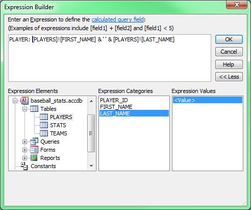 Text Description (click to reveal)
PLAYER: [PLAYERS]![FIRST_NAME] & ’ ’ & [PLAYERS]![LAST_NAME] - When you've finished writing the expression, click OK to dismiss the Expression Builder.
- The LAST_NAME column is now redundant, so remove it from the design grid as described above.
- Run the query and confirm that the name values concatenated properly.
C. Sorting by a field not included in the output
Suppose you wanted to sort this list by the last name, then first name, and then by the number of RBI. This would make it easier to look at each player's best seasons in terms of RBI production.
- In Design View, double-click on LAST_NAME, then FIRST_NAME to add them back to the design grid.
- Choose the Ascending option in the Sort cell for both the LAST_NAME and FIRST_NAME fields.
- Again, these fields are redundant with the addition of the PLAYER expression. Uncheck the Show checkbox for both fields so that they are not included in the query results. Note that the ordering of the Sort fields in the design grid is important. The results are sorted first based on the left-most Sort field, then by the next Sort field, then the next, etc.
- If necessary, click on the thin gray selection bar above the RBI field in the design grid to select that column. Click and drag to the right so that it is moved to the right of the _NAME columns.
- Choose Descending as the Sort option for the RBI field.
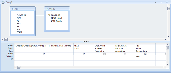
- Run the query and confirm that the records sorted properly. (Hank Aaron should be listed first.)
D. Performing an outer join
If you were to count the number of players being displayed by our query, you'd find that there are 10 (PLAYER_IDs 1 through 10).
- Open the PLAYERS table and note that there is a player (Alex Rodriguez, PLAYER_ID 11) who is not appearing in the query output.
- Now open the STATS table and note that there are records with a PLAYER_ID of 12, but no matching player with that ID in the PLAYERS table. These records aren't included in the query output either.
The unmatched records in these tables aren't appearing in the query output because the join between the tables is an inner join. Inner joins display data only from records that have a match in the join field values.
To display data from the unmatched records, we need to use an outer join.
Close the tables. - Leave Query1 open, as we'll come back to it in a moment. Create a new query (Create > Query Design).
- Add the PLAYERS and STATS tables to the design grid of the new query, and then close the Show Table dialog.
- Create a join between the PLAYER_ID fields.
- Add the PLAYER_ID, FIRST_NAME and LAST_NAME fields from the PLAYERS table to the design grid.
- Add the PLAYER_ID, YEAR and HR fields from the STATS table.
- Choose the Sort Ascending option for the PLAYER_ID field (the one from the STATS table) and the YEAR field.
- Right-click on the line connecting the PLAYER_ID fields and select Join Properties.
Note that join option 1 is currently selected (only include rows where the joined fields from both tables are equal). - Click on the Include ALL records from 'PLAYERS' option, then click OK. Whether this is option 2 or 3 will depend on whether you clicked and dragged from PLAYERS to STATS or from STATS to PLAYERS. In any case, note that the line connecting the key fields is now an arrow pointing from the PLAYERS table to the STATS table.
- Test the query. The query outputs PLAYER_ID 11 (at the top) in addition to 1 through 10. Because there are no matching records for PLAYER_ID 11 in the STATS table, the STATS columns in the output contain NULL values.
- Return to Design View and bring up the Join Properties dialog again. This time choose option 3, so that all records from the STATS table will be shown, then click OK. The arrow connecting the key fields is now reversed, pointing from the right (STATS) table to the left (PLAYERS) table.
- Test the query. If you scroll to the bottom, you'll see that the query outputs the stats for PLAYER_ID 12. This player has no match in the PLAYERS table, so the PLAYERS columns in the output contain NULL values.
- Close Query2 without saving.
E. Performing a cross join
Another type of join that we'll use later when we write spatial queries in PostGIS is the cross join, which produces the Cartesian, or cross, product of the two tables. If one table has 10 records and the other 5, the cross join will output 50 records.
- Create another new query adding the PLAYERS and TEAMS tables to the design grid. You won't see a join line automatically connecting fields in the two tables (they don't share a field in common). This lack of a line connecting the tables is actually what we want, as it will cause a cross join to be performed.
- Add the PLAYER_ID field from the PLAYERS table and the ABBREV field from the TEAMS table to the design grid.
- Test the query. Note that the query outputs 275 records (the product of 11 players and 25 teams). Each record represents a different player/team combination.
- Close Query2 without saving.
The usefulness of this kind of join may not be obvious given this particular example. For a better example, imagine a table of products that includes each product's retail price and a table of states and their sales taxes. Using a cross join between these two tables, you could calculate the sales price of each product in each state.
F. Creating a query with multiple joins
Finally, let's put together a query that joins together data from 3 tables.
- Create another new query adding the PLAYERS, STATS and TEAMS tables to the design grid.
- Create the PLAYER_ID-based join between the PLAYERS and STATS tables.
- Click on the TEAM field in the STATS table and drag over to the ABBREV field in the TEAMS table, (recall that field names do not have to match when creating a join).
- Add the FIRST_NAME and LAST_NAME fields from the PLAYERS table, the YEAR and HR fields from the STATS table and the CITY and NICKNAME fields from the TEAMS table.
- Test the query.
- Close Query2 without saving.
In this way, it is possible to create queries containing several joins. However, in a real database, you are likely to notice a drop in performance as the number of joins increases.
In this section, we saw how to pull together data from two or more related tables, how to concatenate values from two text fields, and how to sort query records based on fields not included in the output. This enabled us to produce a much more user- friendly output than we had at the end of the previous section. In the next section, we'll further explore the power of SELECT queries by compiling career statistics and calculating new statistics on the fly from values stored in the STATS table.
Aggregating Data
Aggregating Data
One of the beauties of SQL is in its ability to construct groupings from the values in a table and produce summary statistics for those groupings. In our baseball example, it is quite easy to calculate each player's career statistics, seasons played, etc. Let's see how this type of query is constructed by calculating each player's career RBI total.
A. Adding a GROUP BY clause to calculate the sum of values in a field
- Return to Design View (your Query 1 design should still be there) and remove the LAST_NAME and FIRST_NAME fields from the design grid.
- With the Design tab selected, click on the Totals button on the right side of the Ribbon in the Show/Hide group of buttons. This will add a Total row to the design grid with each field assigned the value Group By.
- Click in the Total cell under the RBI column and select Sum from the drop-down list (note the other options available on this list, especially Avg, Max, and Min).
- Grouping by both the player's name and the year won't yield the desired results, since the data in the STATS table are essentially already grouped in that way. We want the sum of the RBI values for each player across all years, so remove the YEAR column from the design grid and remove the >99 from the Criteria row.
- Modify the query so that the results are sorted from highest career RBI total to lowest.
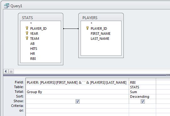
- Run the query and note that the RBI column name defaults to 'SumOfRBI'. You can override this by returning to Design View and entering a custom name (such as CareerRBI) and a colon before the RBI field name (following the PLAYER field example).
B. Use the Expression Builder to perform a calculation based on multiple field values
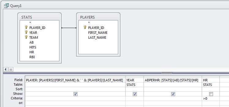
Home run hitters are often compared based on the frequency of their home run hitting (i.e., 'Player X averages a home run every Y times at bat'). Let's calculate this value for each player and season.
- Click on the Totals button on the query Design toolbar to toggle off the Total row in the design grid.
- Remove the RBI field from the design grid.
- Add the YEAR field to the design grid.
- In the third column (which is empty), right-click in the Field cell and click on Build to pull up the Expression Builder as done earlier.
- Navigate inside the database and click on STATS to see a list of its fields.
- Use the GUI to build the following expression:
ABPERHR: [STATS]![AB]/[STATS]![HR]
- If a player had 0 HR in a season, this calculation will generate an error (can't divide by 0, test the query and look for #Div/0!), so add the HR field to the design grid, add >0 to its Criteria cell and uncheck its Show checkbox.
- Sort the query results (not shown below) by the ABPERHR value from lowest to highest (since low values are better than high values).
- Run the query and note that the calculated values include several digits after the decimal point. These digits aren't really necessary, so return to Design View, right-click on the ABPERHR field and select Properties.
- A Property Sheet pane will appear on the right side of the window. Select Fixed from the Format drop-down list and set the Decimal Places value to 1.
- Re-run the query and confirm that you get the desired results.
SELECT Query Syntax
SELECT Query Syntax
Hopefully, you've found the MS-Access query builder to be helpful in learning the basics of retrieving data from a database. As you move forward, it will become important for you to learn some of the syntax details (i.e., how to write the statements you saw in SQL View without the aid of a graphical query builder). That will be the focus of this part of the lesson.
A. The SELECT clause
All SELECT queries begin with a SELECT clause whose purpose is to specify which columns should be retrieved. The desired columns are separated by commas. Our first query in this lesson had a SELECT clause that looked like the following:
SELECT STATS.PLAYER_ID, STATS.HR, STATS.RBI
Note that each column name is preceded by the name of its parent table, followed by a dot. This is critical when building a query involving joins and one of the desired columns is found in multiple tables. Including the parent table eliminates any confusion the SQL interpreter would have in deciding which column should be retrieved. However, you should keep in mind that the table name can be omitted when the desired column is unambiguous. For example, because our simple query above is only retrieving data from one table, the SELECT clause could be reduced to:
SELECT PLAYER_ID, HR, RBI
Selecting all columns
The easiest way to retrieve data from a table is to substitute the asterisk character (*) for the list of columns:
SELECT *
This will retrieve data from all of the columns. While it's tempting to use this syntax because it's so much easier to type, you should be careful to do so only when you truly want all of the data held in the table or when the table is rather small. Retrieving all the data from a table can cause significant degradation in the performance of an SQL-based application, particularly when the data is being transmitted over the Internet. Grab only what you need!
Case sensitivity in SQL
Generally speaking, SQL is a case-insensitive language. You'll find that the following SELECT clause will retrieve the same data as the earlier ones:
SELECT player_id, hr, rbi
Why did I say "generally speaking?" There are some RDBMS that are case sensitive depending on the operating system they are installed on. Also, some RDBMS have administrative settings that make it possible to turn case sensitivity on. For these reasons, I suggest treating table and column names as if they are case sensitive.
On the subject of case, one of the conventions followed by many SQL developers is to capitalize all of the reserved words (i.e., the words that have special meaning in SQL) in their queries. Thus, you'll often see the words SELECT, FROM, WHERE, etc., capitalized. You're certainly not obligated to follow this convention, but doing so can make your queries more readable, particularly when table and column names are in lower or mixed case.
Finally, recall that we renamed our output columns (assigned aliases) in some of the earlier query builder exercises by putting the desired alias and a colon in front of the input field name or expression. Doing this in the query builder results in the addition of the AS keyword to the query's SELECT clause, as in the following example:
SELECT PLAYER_ID, HR AS HomeRuns, RBI
B. The FROM clause
The other required clause in a SELECT statement is the FROM clause. This specifies the table(s) containing the columns specified in the SELECT clause. In the first queries we wrote, we pulled data from a single table, like so:
SELECT STATS.PLAYER_ID, STATS.HR, STATS.RBI FROM STATS
Or, omitting the parent table from the column specification:
SELECT PLAYER_ID, HR, RBI FROM STATS
The FROM clause becomes a bit more complicated when combining data from multiple tables. The Access query builder creates an explicit inner join by default. Here is the code for one of our earlier queries:
SELECT PLAYERS.FIRST_NAME, PLAYERS.LAST_NAME, STATS.YEAR, STATS.RBI
FROM PLAYERS INNER JOIN STATS ON PLAYERS.PLAYER_ID = STATS.PLAYER_ID
An inner join like this one causes a row-by-row comparison to be conducted between the two tables looking for rows that meet the criterion laid out in the ON predicate (in this case, that the PLAYER_ID value in the PLAYERS table is the same as the PLAYER_ID value in the STATS table). When a match is found, a new result set is produced containing all of the columns listed in the SELECT clause. If one of the tables has a row with a join field value that is not found in the other table, that row would not be included in the result.
We also created a couple of outer joins to display data from records that would otherwise not appear in an inner join. In the first example, we chose to include all data from the left table and only the matching records from the right table. That yielded the following code:
SELECT [PLAYERS]![FIRST_NAME] & ' ' & [PLAYERS]![LAST_NAME] AS PLAYER, STATS.YEAR, STATS.RBI

    FROM STATS LEFT JOIN PLAYERS ON STATS.PLAYER_ID = PLAYERS.PLAYER_ID
Note that the only difference between this FROM clause and the last is that the INNER keyword was changed to the word LEFT. As you might be able to guess, our second outer join query created code that looks like this:
SELECT [PLAYERS]![FIRST_NAME] & ' ' & [PLAYERS]![LAST_NAME] AS PLAYER, STATS.YEAR, STATS.RBI

    FROM STATS RIGHT JOIN PLAYERS ON STATS.PLAYER_ID = PLAYERS.PLAYER_ID
Here the word LEFT is replaced with the word RIGHT. In practice, RIGHT JOINs are more rare than LEFT JOINs since it's possible to produce the same results by swapping the positions of the two tables and using a LEFT JOIN. For example:
SELECT [PLAYERS]![FIRST_NAME] & ' ' & [PLAYERS]![LAST_NAME] AS PLAYER, STATS.YEAR, STATS.RBI

    FROM PLAYERS LEFT JOIN STATS ON STATS.PLAYER_ID = PLAYERS.PLAYER_ID
Recall that the cross join query we created was characterized by the fact that it had no line connecting key fields in the two tables. As you might guess, this translates to a FROM clause that has no ON predicate:
SELECT STATS.PLAYER_ID, TEAMS.ABBREV

    FROM STATS, TEAMS;
In addition to lacking an ON predicate, the clause also has no form of the word JOIN. The two tables are simply separated by commas.
Finally, we created a query involving two inner joins. Here is how that query was translated to SQL:
SELECT PLAYERS.FIRST_NAME, PLAYERS.LAST_NAME, STATS.YEAR, STATS.HR, TEAMS.CITY, TEAMS.NICKNAME

    FROM (PLAYERS INNER JOIN STATS ON PLAYERS.PLAYER_ID = STATS.PLAYER_ID) INNER JOIN TEAMS ON STATS.TEAM = TEAMS.ABBREV;
The first join is enclosed in parentheses to control the order in which the joins are carried out. Like in algebra, operations in parentheses are carried out first. The result of the first join then participates in the second join.
C. The WHERE clause
As we saw earlier, it is possible to limit a query's result to records meeting certain criteria. These criteria are spelled out in the query's WHERE clause. This clause includes an expression that evaluates to either True or False for each row. The "True" rows are included in the output; the "False" rows are not. Returning to our earlier examples, we used a WHERE clause to identify seasons of 100+ RBIs:
SELECT STATS.PLAYER_ID, STATS.YEAR, STATS.RBI

    FROM STATS

    WHERE STATS.RBI > 99
As with the specification of columns in the SELECT clause, columns in the WHERE clause need not be prefaced by their parent table if there is no confusion as to where the columns are coming from.
This statement exemplifies the basic column-operator-value pattern found in most WHERE clauses. The most commonly used operators are:
| Operator | Description |
|---|---|
| = | equals |
| <> | not equals |
| > | greater than |
| >= | greater than or equal to |
| < | less than |
| <= | less than or equal to |
| BETWEEN | within a value range |
| LIKE | matching a search pattern |
| IN | matching an item in a list |
The usage of most of these operators is straightforward. But let's talk for a moment about the LIKE and IN operators. LIKE is used in combination with the wildcard character (the * character in Access and most other RDBMS, but the % character in some others) to find rows that contain a text string pattern. For example, the clause WHERE FIRST_NAME LIKE 'B*' would return Babe Ruth and Barry Bonds. WHERE FIRST_NAME LIKE '*ar*' would return Barry Bonds and Harmon Killebrew. WHERE FIRST_NAME LIKE '*ank' would return Hank Aaron and Frank Robinson.
Note:
Text strings like those in the WHERE clauses above must be enclosed in quotes. Single quotes are recommended, though double quotes will also work in most databases. This is in contrast to numeric values, which should not be quoted. The key point to consider is the data type of the column in question. For example, zip code values may look numeric, but if they are stored in a text field (as they should be because some begin with zeroes), they must be enclosed in quotes.
The IN operator is used to identify values that match an item in a list. For example, you might find seasons compiled by members of the Giants franchise (which started in New York and moved to San Francisco) using a WHERE clause like this:
WHERE TEAM IN ('NYG', 'SFG')
Finally, remember that WHERE clauses can be compound. That is, you can evaluate multiple criteria using the AND and OR operators. The AND operator requires that both the expression on the left and the expression on the right evaluate to True, whereas the OR operator requires that at least one of the expressions evaluates to True. Here are a couple of simple illustrations:
WHERE TEAM = 'SFG' AND YEAR > 2000
WHERE TEAM = 'NYG' OR TEAM = 'SFG'
Sometimes WHERE clauses require parentheses to ensure that the filtering logic is carried out properly. One of the queries you were asked to write earlier sought to identify 100+ RBI seasons compiled before 1960 or after 1989. The SQL generated by the query builder looks like this:
SELECT STATS.PLAYER_ID, STATS.YEAR, STATS.RBI

    FROM STATS

    WHERE (((STATS.YEAR)>1989) AND ((STATS.RBI)>99)) OR (((STATS.YEAR)<1960) AND ((STATS.RBI)>99));
It turns out that this statement is more complicated than necessary for a couple of reasons. The first has to do with the way I instructed you to build the query:
This resulted in the RBI>99 criterion inefficiently being added to the query twice. A more efficient approach would be to merge the two-year criteria into a single row in the design grid, as follows:
This yields a more efficient version of the statement:
SELECT STATS.PLAYER_ID, STATS.YEAR, STATS.RBI

    FROM STATS

    WHERE (((STATS.YEAR)>1989 Or (STATS.YEAR)<1960) AND ((STATS.RBI)>99));
It is difficult to see, but this version puts a set of parentheses around the two year criteria so that the condition of being before 1960 or after 1989 is evaluated separately from the RBI condition.
One reason the logic is difficult to follow is because the query builder adds parentheses around each column specification. Eliminating those parentheses and the table prefixes produces a more readable query:
SELECT PLAYER_ID, YEAR, RBI

    FROM STATS

    WHERE (YEAR>1989 Or YEAR<1960) AND RBI>99;
D. The GROUP BY clause
The GROUP BY clause was generated by the query builder when we calculated each player's career RBI total:
SELECT LAST_NAME, FIRST_NAME, Sum(RBI) AS SumOfRBI

    FROM STATS

    GROUP BY LAST_NAME, FIRST_NAME;
The idea behind this type of query is that you want the RDBMS to find all of the unique values (or value combinations) in the field (or fields) listed in the GROUP BY clause and include each in the result set. When creating this type of query, each field in the GROUP BY clause must also be listed in the SELECT clause. In addition to the GROUP BY fields, it is also common to use one of the SQL aggregation functions in the SELECT clause to produce an output column. The function we used to calculate the career RBI total was Sum(). Other useful aggregation functions include Max(), Min(), Avg(), Last(), First() and Count(). Because the Count() function is only concerned with counting the number of rows associated with each grouping, it doesn't really matter which field you plug into the parentheses. Frequently, SQL developers will use the asterisk rather than some arbitrary field. This modification to the query will return the number of years in each player's career, in addition to the RBI total:
SELECT LAST_NAME, FIRST_NAME, Sum(RBI) AS SumOfRBI, Count(*) AS Seasons

    FROM STATS

    GROUP BY LAST_NAME, FIRST_NAME;
Note: In actuality, this query would over count the seasons played for players who switched teams mid-season (e.g., Mark McGwire was traded in the middle of 1997 and has a separate record in the STATS table for each team). We'll account for this problem using a sub-query later in the lesson.
E. The ORDER BY clause
The purpose of the ORDER BY clause is to specify how the output of the query should be sorted. Any number of fields can be included in this clause, so long as they are separated by commas. Each field can be followed by the keywords ASC or DESC to indicate ascending or descending order. If this keyword is omitted, the sorting is done in an ascending manner. The query below sorts the seasons in the STATS table from the best RBI total to the worst:
SELECT PLAYER_ID, YEAR, RBI

    FROM STATS

    ORDER BY RBI DESC;
That concludes our review of the various clauses found in SELECT queries. You're likely to memorize much of this syntax if you're called upon to write much SQL from scratch. However, don't be afraid to use the Access query builder or other GUIs as an aid in producing SQL statements. I frequently take that approach when writing database-related PHP scripts. Even though the data is actually stored in a MySQL database, I make links to the MySQL tables in Access and use the query builder to develop the queries I need. That workflow (which we'll explore in more depth later in the course) is slightly complicated by the fact that the flavor of SQL produced by Access differs slightly from industry standards. We'll discuss a couple of the important differences in the next section.
Differences Between MS-Access and Standard SQL
Differences Between MS-Access and Standard SQL
If you plan to use the SQL generated by the Access query builder in other applications as discussed on the previous page, you'll need to be careful of some of the differences between Access SQL and other RDBMS.
A. Table/Column Specification in the Expression Builder
We used the Expression Builder to combine the players' first and last names, and later to calculate their home run per at-bat ratio. Unfortunately, the Expression Builder specifies table/column names in a format that is unique to Access. Here is a simplified version of the HR/AB query that doesn't bother including names from the PLAYERS table:
SELECT STATS.PLAYER_ID, STATS.YEAR, [STATS]![AB]/[STATS]![HR] AS ABPERHR

	FROM STATS;
The brackets and exclamation point used in this expression is non-standard SQL and would not work outside of Access. A safer syntax would be to use the same table.column notation used earlier in the SELECT clause:
SELECT STATS.PLAYER_ID, STATS.YEAR, STATS.AB/STATS.HR AS ABPERHR

	FROM STATS;
Or, to leave out the parent table name altogether:
SELECT PLAYER_ID, YEAR, AB/HR AS ABPERHR

	FROM STATS;
Note that this modified syntax will work in Access.
B. String Concatenation
In our queries that combined the players' first and last names, the following syntax was used:
SELECT [PLAYERS]![FIRST_NAME] & ' ' & [PLAYERS]![LAST_NAME]....
As mentioned above, columns should be specified using the table.column notation rather than with brackets and exclamation points. In addition to the different column specification, the concatenation itself would also be done differently in other RDBMS. While Access uses the & character for concatenation, the concatenation operator in standard SQL is ||. However, there is considerable variation in the adherence to this standard. For a comparison of a number of the major RDBMS [2], see http://troels.arvin.dk/db/rdbms/#functions-concat.
Note:
One of the points of comparison in the linked page is whether or not there is automatic casting of values. All this is getting at is what happens if the developer tries to concatenate a string with some other data type (say, a number). Some SQL implementations will automatically cast, or convert, the number to a string. Others are less flexible and require the developer to perform such a cast explicitly.
Subqueries
Subqueries
There comes a time when every SQL developer has a problem that is too difficult to solve using only the methods we've discussed so far. In our baseball stats database, difficulty arises when you consider the fact that players who switch teams mid-season have a separate row for each team in the STATS table. For example, Mark McGwire started the 1997 season with OAK, before being traded to and spending the rest of that season with STL. The STATS table contains two McGwire-1997 rows; one for his stats with OAK and one for his stats with STL.
If you wanted to identify each player's best season (in terms of batting average, home runs or runs batted in), you wouldn't be able to do a straight GROUP BY on the player's name or ID because that would not account for the mid-season team switchers. What's needed in this situation is a multistep approach that first computes each player's yearly aggregated stats, then identifies the maximum value in that result set.
A novice's approach to this problem would be to output the results from the first query to a new table, then build a second query on top of the table created by the first. The trouble with this approach is that it requires re-running the first query each time the STATS table changes.
A more ideal solution to the problem can be found through the use of a subquery. Let's have a look at how to build a subquery in Access.
A. Building a query on top of another saved query
- Create a new query and add the STATS table to the design canvas.
- Click on the Totals button to add the Total row to the design grid.
- Bring the following fields down into the design grid: PLAYER_ID, YEAR, AB, HITS, HR, RBI, and TEAM.
- Set the value in the Total cell to Group By for the PLAYER_ID and YEAR fields.
- Set the value in the Total cell to Sum for the AB, HITS, HR, and RBI fields.
- Set the value in the Total cell to Count for the TEAM field. These settings specify that we want to group by the player ID and year, sum the player's stats across each player/year grouping, and include a count of the number of teams the player played for each year.
- Run the query and confirm that it produces 227 records. (Compare that against the number of records in the STATS table. Do you understand why there is a difference?)
- Save the query as STATS_AGGR.
- Now, create a new query. In the Show Table dialog, double-click on PLAYERS to add it to the design canvas.
- Next, in the Show Table dialog, switch from the Tables tab to the Queries tab and double-click on STATS_AGGR to add it to the design canvas. Let's identify each player's best season in terms of home runs.
- Again, click on the Totals button.
- Bring down to the design grid the FIRST_NAME and LAST_NAME fields from the PLAYERS table and SumOfHR from the STATS_AGGR query.
- Confirm that the value in the Total cell is set to Group By for the FIRST_NAME and LAST_NAME fields.
- Set the value in the Total cell for the SumOfHR field to Max.
- Save this query as QueryBasedOnAQuery.
B. Building a query within another query.
- Switch to the SQL View of the QueryBasedOnAQuery query (sorry about that). Note that an inner join is conducted between PLAYERS and STATS_AGGR. When Access executes this query, it needs to first evaluate the SQL stored in the STATS_AGGR query before it can join that result set to PLAYERS. In your mind, you can imagine replacing the STATS_AGGR part of the PLAYERS INNER JOIN STATS_AGGR expression with the SQL stored in STATS_AGGR. In fact, our next step will be to literally replace STATS_AGGR with its SQL code.
- Re-open the STATS_AGGR query and switch to SQL View.
- Highlight and copy the SQL (leave behind the trailing semi-colon).
- Return to the SQL View of the QueryBasedOnAQuery query.
- Remove the STATS_AGGR from the PLAYERS INNER JOIN STATS_AGGR and paste in the code on your clipboard.
- Insert parentheses around the code you just pasted and add AS STATS_AGG after the closing parenthesis. Note that we're giving the subquery an alias of STATS_AGG to avoid confusion with the saved query with the name STATS_AGGR.
- Replace the query's references to STATS_AGGR with STATS_AGG, (there is one reference to STATS_AGGR in the SELECT clause and one in the ON clause). Your query should look like this:
SELECT PLAYERS.FIRST_NAME, PLAYERS.LAST_NAME, Max(STATS_AGG.SumOfHR) AS MaxOfSumOfHR FROM PLAYERS INNER JOIN (SELECT STATS.PLAYER_ID, STATS.YEAR, Sum(STATS.AB) AS SumOfAB, Sum(STATS.HITS) AS SumOfHITS, Sum(STATS.HR) AS SumOfHR, Sum(STATS.RBI) AS SumOfRBI, Count(STATS.TEAM) AS CountOfTEAM FROM STATS GROUP BY STATS.PLAYER_ID, STATS.YEAR) AS STATS_AGG ON PLAYERS.PLAYER_ID = STATS_AGG.PLAYER_ID GROUP BY PLAYERS.FIRST_NAME, PLAYERS.LAST_NAME; - Test the query. It should report the highest single-season home run total for each player.
This approach is a bit more complicated than the first, since it cannot be carried out with the graphical Query Builder. However, the advantage is that all of the code involved can be found in one place, and you don't have a second intermediate query cluttering the database's object list.
This completes the material on retrieving data from an RDBMS using SELECT queries. In the next section, you'll be posed a number of questions that will test your ability to write SELECT queries on your own.
Project 1: Writing SQL SELECT Queries
Project 1: Writing SQL SELECT Queries
To demonstrate that you've learned the material from Lesson 1, please build queries in your Access database for each of the problems posed below. Some tips:
- Remember that players who played for multiple teams in the same season (i.e., were traded mid-season) will have a separate row in the STATS table for each team-year combination.
- Even if the requested query does not explicitly ask for player names in the output, please include names to make the output more informative.
- Some of the problems require the use of sub-queries. You will receive equal credit whether you choose to embed your sub-query within the larger query or save your sub-query separately and build your final query upon that saved sub-query.
- You should treat the words 'season' and 'year' in the problems below as synonymous.
Here are the problems to solve:
- Display all records/fields from the STATS table for players on the San Francisco Giants (SFG).
- Output the batting average (HITS divided by AB) for each player and season. Format this value so that exactly 3 digits appear after the decimal point.
For example, Babe Ruth had a batting average of .200 in 1914 (2 hits in 10 at-bats).
- Display all records/fields from the STATS table along with the names of the players in the format “Ruth, Babe”.
- Calculate the number of seasons each player played for each of his teams. (Players who were on two teams in the same season can be counted as having played for both teams.)
For example, Mark McGwire played 12 seasons for the Oakland Athletics and 5 seasons for the St Louis Cardinals (1997 being counted for both teams).
- List the players based on the number of home runs hit in their rookie (first) seasons, from high to low.
For example, Frank Robinson hit 38 home runs in his rookie season of 1956.
- Display the names (only the names, with no duplicates) of players who played in New York (any team beginning with 'NY').
- Sort the players by the number of seasons played (high to low). (Do not double-count in cases in which a player switched teams mid-season.)
For example, Sammy Sosa played 18 seasons, with 1989, which he split between CHW and TEX counted as 1 season, not 2.
- Sort the players by their career batting average (career hits divided by career at-bats, high to low).
For example, Harmon Killebrew had a career batting average of .256 (2086 hits in 8147 at-bats).
- Sort the players by their number of seasons with 100 or more RBI (high to low).
For example, Hank Aaron had 100 or more RBI in a season 11 times.
- Sort the players based on the number of years between their first and last seasons of 40 or more HR (from most to least).
For example, Willie Mays had his first 40-HR season in 1954 and his last in 1965, a difference of 11 years.
Name your queries so that it's easy for me to identify them (e.g., Proj1_1 through Proj1_10).
Deliverables
This project is one week in length. Please refer to the Canvas Calendar for the due date.
- Upload your Access database (.accdb file) containing your solutions to the 10 query exercises above to the Project 1 Dropbox. (100 of 100 points)
- Complete the Lesson 1 quiz.
Lesson 2: Relational Database Concepts and Theory
Overview
Overview
Now that you've gotten a taste of the power provided by relational databases to answer questions, let's shift our attention to the dirty work: designing, implementing, populating and maintaining a database.
Objectives
At the successful completion of this lesson, students should be able to:
- design a relational database and depict that design through an entity-relationship diagram;
- create new tables in MS-Access;
- develop and execute insert, update and delete queries in MS-Access;
- describe what is meant by 1st, 2nd and 3rd normal forms in database design;
- explain the concept of referential integrity.
Questions?
If you have any questions now or at any point during this week, please feel free to post them to the Lesson 2 Discussion Forum.
Checklist
Checklist
Lesson 2 is one week in length, see the Canvas Calendar for specific due dates. To finish this lesson, you must complete the activities listed below:
- Work through Lesson 2.
- Complete Project 2 and upload its deliverables to the Project 2 Dropbox.
- Complete the Lesson 2 Quiz.
Relational DBMSs Within The Bigger Picture
Relational DBMSs Within The Bigger Picture
Before digging deeper into the workings of relational database management systems (RDBMSs), it's a good idea to take a step back and look briefly at the history of the relational model and how it fits into the bigger picture of DBMSs in general. The relational model of data storage was originally proposed by an IBM employee named Edgar Codd in the early 1970s. Prior to that time, computerized data storage techniques followed a "navigational" model that was not well suited to searching. The ground-breaking aspect of Codd's model was the allocation of data to separate tables, all linked to one another by keys - values that uniquely identify particular records. The process of breaking data into multiple tables is referred to as normalization.
If you do much reading on the relational model, you're bound to come across the terms relation, attribute, and tuple. While purists would probably disagree, for our purposes you can consider relation to be synonymous with table, attribute with the terms column and field, and tuple with the terms row and record.
SQL, which we started learning about in Lesson 1, was developed in response to Codd's relational model. Today, relational databases built around SQL dominate the data storage landscape. However, it is important to recognize that the relational model is not the only ballgame in town. Object-oriented databases [3] arose in the 1980s in parallel with object-oriented programming languages. Some of the principles of object-oriented databases (such as classes and inheritance) have made their way into most of today's major RDBMSs, so it is more accurate to describe them as object-relational hybrids.
More recently, a class of DBMSs that deviate significantly from the relational model has developed. These NoSQL databases [4] seek to improve performance when dealing with large volumes of data (often in web-based applications). Essentially, these systems sacrifice some of the less critical functions found in an RDBMS in exchange for gains in scalability and performance.
Database Design Concepts
Database Design Concepts
A. Database design concepts
When building a relational database from scratch, it is important that you put a good deal of thought into the process. A poorly designed database can cause a number of headaches for its users, including:
- loss of data integrity over time
- inability to support needed queries
- slow performance
Entire courses can be spent on database design concepts, but we don't have that kind of time, so let's just focus on some basic design rules that should serve you well. A well-designed table is one that:
- seeks to minimize redundant data
- represents a single subject
- has a primary key (a field or set of fields whose values will uniquely identify each record in the table)
- does not contain multi-part fields (e.g., "302 Walker Bldg, University Park, PA 16802")
- does not contain multi-valued fields (e.g., an Author field shouldn't hold values of the form "Jones, Martin, Williams")
- does not contain unnecessary duplicate fields (e.g., avoid using Author1, Author2, Author3)
- does not contain fields that rely on other fields (e.g., don't create a Wage field in a table that has PayRate and HrsWorked fields)
B. Normalization
The process of designing a database according to the rules described above is formally referred to as normalization. All database designers carry out normalization, whether they use that term to describe the process or not. Hardcore database designers not only use the term normalization, they're also able to express the extent to which a database has been normalized:
- First normal form (1NF) describes a database whose tables represent distinct entities, have no duplicative columns (e.g., no Author1, Author2, Author3), and have a column or columns that uniquely identify each row (i.e., a primary key). Databases meeting these requirements are said to be in first normal form.
- Second normal form (2NF) describes a database that is in 1NF and also avoids having non-key columns that are dependent on a subset of the primary key. It's understandable if that seems confusing, have a look at this simple example [5] [www.1keydata.com/database-normalization/second-normal-form-2nf.php]
In the example, CustomerID and StoreID form a composite key - that is, the combination of the values from those columns uniquely identifies the rows in the table. In other words, only one row in the table will have a CustomerID of 1 together with a StoreID of 1, only one row will have a CustomerID of 1 together with a StoreID of 3, etc. The PurchaseLocation column depends on the StoreID column, which is only part of the primary key. As shown, the solution to putting the table in 2NF is to move the StoreID-PurchaseLocation relationship into a separate table. This should make intuitive sense as it spells out the PurchaseLocation values just once rather than spelling them out repeatedly. - Third normal form (3NF) describes a database that is in 2NF and also avoids having columns that derive their values from columns other than the primary key. The wage field example mentioned above is a clear violation of the 3NF rule.
In most cases, normalizing a database so that it is in 3NF is sufficient. However, it is worth pointing out that there are other normal forms including Boyce-Codman normal form (BCNF, or 3.5NF), fourth normal form (4NF) and fifth normal form (5NF). Rather than spend time going through examples of these other forms, I encourage you to simply keep in mind the basic characteristics of a well-designed table listed above. If you follow those guidelines carefully, in particular, constantly being on the lookout for redundant data, you should be able to reap the benefits of normalization.
Generally speaking, a higher level of normalization results in a higher number of tables. And as the number of tables increases, the costs of bringing together data through joins increases as well, both in terms of the expertise required in writing the queries and in the performance of the database. In other words, the normalization process can sometimes yield a design that is too difficult to implement or that performs too slowly. Thus, it is important to bear in mind that database design is often a balancing of concerns related to data integrity and storage efficiency (why we normalize) versus concerns related to its usability (getting data into and out of the database).
Earlier, we talked about city/state combinations being redundant with zip code. That is a great example of a situation in which de-normalizing the data might make sense. I have no hard data on this, but I would venture to say that the vast majority of relational databases that store these three attributes keep them all together in the same table. Yes, there is a benefit to storing the city and state names once in the zip code table (less chance of a misspelling, less disk space used). However, my guess is that the added complexity of joining the city/state together with the rest of the address elements outweighs that benefit to most database designers.
C. Example scenario
Let's work through an example design scenario to demonstrate how these rules might be applied to produce an efficient database. Ice cream entrepreneurs Jen and Barry have opened their business and now need a database to track orders. When taking an order, they record the customer's name, the details of the order such as the flavors and quantities of ice cream needed, the date the order is needed, and the delivery address. Their database needs to help them answer two important questions:
- Which orders are due to be shipped within the next two days?
- Which flavors must be produced in greater quantities?
A first crack at storing the order information might look like this:
| Customer | Order | DeliveryDate | DeliveryAdd |
|---|---|---|---|
| Eric Cartman | 1 vanilla, 2 chocolate | 12/1/11 | 101 Main St |
| Bart Simpson | 10 chocolate, 10 vanilla, 5 strawberry | 12/3/11 | 202 School Ln |
| Stewie Griffin | 1 rocky road | 12/3/11 | 303 Chestnut St |
| Bart Simpson | 3 mint chocolate chip, 2 strawberry | 12/5/11 | 202 School Ln |
| Hank Hill | 2 coffee, 3 vanilla | 12/8/11 | 404 Canary Dr |
| Stewie Griffin | 5 rocky road | 12/10/11 | 303 Chestnut St |
The problem with this design becomes clear when you imagine trying to write a query that calculates the number of gallons of vanilla that have been ordered. The quantities are mixed with the names of the flavors, and any one flavor could be listed anywhere within the order field (i.e., it won't be consistently listed first or second).
A design like the following would be slightly better:
| Customer | Flavor1 | Qty1 | Flavor2 | Qty2 | Flavor3 | Qty3 | DeliveryDate | DeliveryAdd |
|---|---|---|---|---|---|---|---|---|
| Eric Cartman | vanilla | 1 | chocolate | 2 | 12/1/11 | 101 Main St |
||
| Bart Simpson | chocolate | 10 | vanilla | 10 | strawberry | 5 | 12/3/11 | 202 School Ln |
| Stewie Griffin | rocky road | 1 | 12/3/11 | 303 Chestnut St |
||||
| Bart Simpson | mint chocolate chip | 3 | strawberry | 2 | 12/5/11 | 202 School Ln |
||
| Hank Hill | coffee | 2 | vanilla | 3 | 12/8/11 | 404 Canary Dr |
||
| Stewie Griffin | rocky road | 5 | 12/10/11 | 303 Chestnut St |
This is an improvement because it enables querying on flavors and summing quantities. However, to calculate the gallons of vanilla ordered you would need to sum the values from three fields. Also, the design would break down if a customer ordered more than three flavors.
Slightly better still is this design:
| Customer | Flavor | Qty | DeliveryDate | DeliveryAdd |
|---|---|---|---|---|
| Eric Cartman | vanilla | 1 | 12/1/11 | 101 Main St |
| Eric Cartman | chocolate | 2 | 12/1/11 | 101 Main St |
| Bart Simpson | chocolate | 10 | 12/3/11 | 202 School Ln |
| Bart Simpson | vanilla | 10 | 12/3/11 | 202 School Ln |
| Bart Simpson | strawberry | 5 | 12/3/11 | 202 School Ln |
| Stewie Griffin | rocky road | 1 | 12/3/11 | 303 Chestnut St |
| Hank Hill | coffee | 2 | 12/8/11 | 404 Canary Dr |
| Hank Hill | vanilla | 3 | 12/8/11 | 404 Canary Dr |
| Stewie Griffin | rocky road | 5 | 12/10/11 | 303 Chestnut St |
This design makes calculating the gallons of vanilla ordered much easier. Unfortunately, it also produces a lot of redundant data and spreads a complete order from a single customer across multiple rows.
Better than all of these approaches would be to separate the data into four entities (Customers, Flavors, Orders and Order Items):
| CustID | NameLast | NameFirst | DeliveryAdd |
|---|---|---|---|
| 1 | Cartman | Eric | 101 Main St |
| 2 | Simpson | Bart | 202 School Ln |
| 3 | Griffin | Stewie | 303 Chestnut St |
| 4 | Hill | Hank | 404 Canary Dr |
| FlavorID | Name |
|---|---|
| 1 | vanilla |
| 2 | chocolate |
| 3 | strawberry |
| 4 | rocky road |
| 5 | mint chocolate chip |
| 6 | coffee |
| OrderID | CustID | DeliveryDate |
|---|---|---|
| 1 | 1 | 12/1/11 |
| 2 | 2 | 12/3/11 |
| 3 | 3 | 12/3/11 |
| 4 | 2 | 12/5/11 |
| 5 | 4 | 12/8/11 |
| 6 | 3 | 12/10/11 |
| OrderItemID | OrderID | FlavorID | Qty |
|---|---|---|---|
| 1 | 1 | 1 | 1 |
| 2 | 1 | 2 | 2 |
| 3 | 2 | 2 | 10 |
| 4 | 2 | 1 | 10 |
| 5 | 2 | 3 | 5 |
| 6 | 3 | 4 | 1 |
| 7 | 4 | 5 | 3 |
| 8 | 4 | 3 | 2 |
| 9 | 5 | 6 | 2 |
| 10 | 5 | 1 | 3 |
| 11 | 6 | 4 | 5 |
If one were to implement a design like this in MS-Access, the query needed to display orders that must be delivered in the next 2 days would look like this in the GUI:
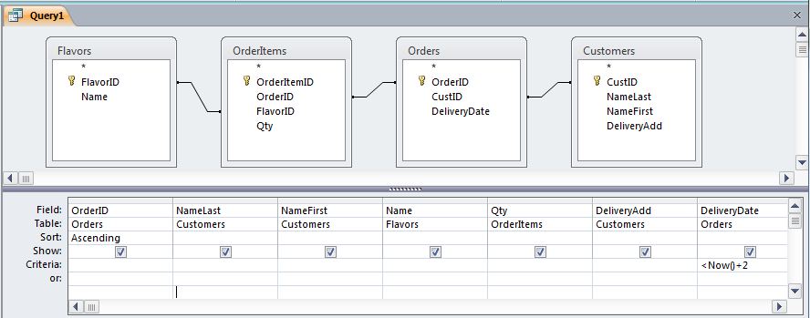
It would produce the following SQL:
If you aren't experienced with relational databases, then such a table join may seem intimidating. You probably won't need to do anything quite so complex in this course. The purpose of this example is two-fold:
- To illustrate that multi-table designs are often preferable to a "one-big-spreadsheet" approach.
- To emphasize the importance of SQL in pulling together data spread across multiple tables to perform valuable database queries.
D. Data modeling
Whether it's just a quick sketch on a napkin or a months-long process involving many stakeholders, the life cycle of any effective database begins with data modeling. Data modeling itself begins with a requirements analysis, which can be more or less formal, depending on the scale of the project. One of the common products of the data modeling process is an entity-relationship (ER) diagram. This sort of diagram depicts the categories of data that must be stored (the entities) along with the associations (or relationships) between them. The Wikipedia entry on ER diagrams is quite good, so I'm going to point you there to learn more:
Entity-relationship model article at Wikipedia [6] [http://en.wikipedia.org/wiki/Entity-relationship_model]
An ER diagram is essentially a blueprint for a database structure. Some RDBMSs provide diagramming tools (e.g., Oracle Designer, MySQL Workbench) and often include the capability of automatically creating the table structure conceptualized in the diagram.
In a GIS context, Esri makes it possible to create new geodatabases based on diagrams authored using CASE (Computer-Aided Software Engineering) tools. This blog post, Using Case tools in Arc GIS 10 [7], [http://blogs.esri.com/esri/arcgis/2010/08/05/using-case-tools-in-arcgis -10/] provides details if you are interested in learning more.
E. Design practice
To help drive these concepts home, here is a scenario for you to consider. You work for a group with an idea for a fun website: to provide a place for music lovers to share their reviews of albums on the 1001 Albums You Must Hear Before You Die list [8]. (All of these albums had been streamable from Radio Romania 3Net [9], but sadly it appears that's no longer the case.)
Spend 15-30 minutes designing a database (on paper, no need to implement it in Access) for this scenario. Your database should be capable of efficiently storing all of the following data:
- Artist
- Album Genre
- Record Label
- Album Comments
- Album
- Track Name
- Reviewer ID
- Track Rating
- Year
- Track Length
- Album Rating
- Track Comments
When you're satisfied with your design, move to the next page and compare yours to mine.
Implementing a Database Design
Implementing a Database Design
There is no one correct design for the music scenario posed on the last page. The figure below depicts one design. Note the FK notation beside some of the fields. FK stands for foreign key and indicates a field whose values uniquely identify rows in another table. There is no way to designate a field as a foreign key in MS-Access. For our purposes, you should just remember that building foreign keys into your database is what will enable you to create the table joins needed to answer the questions you envision your database answering.
Note also the 1 and * labels at the ends of the relationship lines, which indicate the number of times any particular value will appear in the connected field. As shown in the diagram, values in the Albums table's Album_ID field will appear just once; the same values in the associated field in the Tracks table may appear many times (conveyed by the * character). For example, an album with 10 tracks will have its Album_ID value appear in the Albums table just once. That Album_ID value would appear in the Tracks table 10 times. This uniqueness of values in fields is referred to as cardinality.
If you have questions about this design or see ways to improve it, please share your thoughts in the Lesson 2 Discussion Forum.
In this part of the lesson, we'll create and populate some of the tables depicted in the diagram above to give you a sense of how to move from the design phase to the implementation phase of a database project. Table creation is something that can be accomplished using SQL, as we'll see later in the course. Most RDBMSs also make it possible to create tables through a GUI, which is the approach we will take right now.
An integral part of creating a table is defining its fields and the types of data that can be stored in those fields. Here is a list of the most commonly used data types available in Access:
- Text - for strings of up to 255 characters
- Memo - for strings greater than 255 characters
- Number - for numeric data
- AutoNumber - for automatically incremented numeric fields; more on this below
- Yes/No - for holding values of 'Yes' or 'No'; equivalent to the Boolean type in other RDBMSs
- Date/Time - for storing dates and times
Beyond the data type, fields have a number of other properties that are sometimes useful to set. Among these are Default Value which specifies the value the field takes on by default, and Required, which specifies whether or not the field is allowed to contain Null values. It is also possible to specify that a field is the table's primary key (or part of a multi-field primary key).
Perhaps the most commonly set field property is the Field Size. For Text fields this property defaults to a value of 255 characters. This property should be set to a lower value when appropriate, for a couple of reasons. First, it will reduce the size of the database, and secondly, it can serve as a form of data validation (e.g., assigning a Field Size of 2 to a field that will store state abbreviations will ensure that no more than 2 characters are entered).
When dealing with a Number field, the Field Size property is used to specify the type of number:
- Byte - for integers ranging from 0 to 255
- Integer - for integers in the range of roughly +/- 32,000
- Long Integer - for integers in the range of roughly +/- 2 billion
- Single - for real numbers in the range of roughly +/- 1038
- Double - for real numbers in the range of roughly +/- 10308
As with Text fields, it is good practice to choose the smallest possible Field Size for a Number field.
With this background on fields in mind, let's move on to implementing the music database.
A. Create a new table
- Open Access and from the opening screen click on the Blank Database icon.
- In the right-hand panel, browse to your course folder and give the database the name music.accdb.
- Click the Create button to create the new empty database. Access will automatically create and open a blank table called Table1.
- Select View > Design View to begin modifying this table to meet your needs.
- Give the table the name Albums.
The Design View provides a grid for you to specify the names, data types and other properties for the fields (columns) you want to have in your table. Note that the table automatically has a field called ID with a data type of AutoNumber. The field is also designated as the table's Primary Key.
Note: Most RDBMSs offer an auto-incrementing numeric data type like this. It's common for database tables to use arbitrary integer fields as their primary key. If you create a field as this AutoNumber type (or its equivalent in another RDBMS), you need not supply a value for it when adding new records to the table. The software will automatically handle that for you.
- Rename the field from ID to Album_ID.
- Beneath that field, add a new one called Title.
With the 2013 version of MS Access the interface has changed some when it comes to the next two settings. The list of data types has become more streamlined and the way Field Size is set for numeric fields is different. I will indicate below what the differences are.
- Set the Title field's Data Type to Text.
In Access 2013 - set the Title field's Type to Short Text.
- Set its Field Size to 200. (This and several other options are found in the Field Properties section at the bottom of the window, under the General tab. Note that the maximum value allowed for this property is 255 characters.)
In Access 2013 - no need to set this, the Short Text type holds up to 255 characters.
FYI, the "Long Text" option in Access 2013 ("Memo" option in older Access versions) can hold up to a Gigabyte and can be configured to hold Rich Text formatted information.
- Repeat these steps to add the other fields defined for the Albums table:
In Access 2013 - To set the type and size for numeric data, you first choose Number from the Type list, then under the General tab click the FieldSize property box. Click the arrow and choose the desired field size (Integer, Long Integer, Float, etc.).Table 2.8: Albums Table Name Type Album_ID AutoNumber Title Text (200) Artist_ID Long Integer Release_Year Integer Label_ID Long Integer Note:
Try adding a field with a name of Year to see why we used the name Release_Year instead.
- When finished adding fields to the Albums table, click the Save button.
- To add the next table to the database design, click the Create tab, then Table Design.
- Repeat the steps outlined above to define the Artists table with the following fields:
Table 2.9: Artists Table Name Type Artist_ID AutoNumber Artist_Name Text (200) Year_Begin Integer Year_End Integer - Before closing the table, click in the small gray area to the left of the Artist_ID field to select that field then click on the Primary Key button on the ribbon.
- Create the Labels table with the following fields:
Table 2.10: Labels Table Name Type Label_ID AutoNumber Label_Name Text (200) - Set Label_ID as the primary key of the Labels table.
B. Establish relationships between the tables
While it's not strictly necessary to do so, it can be beneficial to spell out the relationships between the tables that you envisioned during the design phase.
- Click on Database Tools > Relationships.
- From the Show Table dialog double-click on each of the tables to add them to the Relationships layout.
- Arrange the tables so that the Albums table appears between the Artists and Labels tables.
- Like you did when building queries earlier, click on the Artist_ID field in the Artists table and drag it to the Artist_ID field in the Albums table. You should see a dialog titled "Edit Relationships".
- Check each of the three boxes: Enforce Referential Integrity, Cascade Update Related Fields, and Cascade Delete Related Records.
Checking these boxes tells Access that you want its help in keeping the values in the Artist_ID field in sync. For example:- Let's say your Artists table has only three records (with Artist_ID values of 1, 2 and 3). If you attempted to add a record to the Albums table with an Artist_ID of 4, Access would stop you, since that value does not exist in the related Artists table.
- If you change an Artist_ID value in the Artists table, all records in the Albums table will automatically have their Artist_ID values updated to match.
- If you delete an artist from the Artists table, the related records in the Albums table will be deleted as well.
- Click the Create button to establish the relationship between Artists and Albums.
- Follow the same steps to establish a relationship between Albums and Labels based on the Label_ID field.
- Save and Close the Relationships window.
With your database design implemented, you are now ready to add records to your tables.
Adding Records to a Table
Adding Records to a Table
Records may be added to tables in three ways: manually through the table GUI, using an SQL INSERT query to add a single record, and using an INSERT query to add multiple records in bulk.
A. Adding records manually
This method is by far the easiest, but also the most tedious. It is most suitable for populating small tables.
- Double-click on the Labels table in the object list on the left side of the window to open it in Datasheet mode.
- Try entering a value in the Label_ID field. You're not able to because that field was assigned a data type of AutoNumber.
- Tab to the Label_Name field, and enter Capitol. While typing, note the pencil icon in the gray selection box to the left of the record. This indicates that you are editing the record (it may be yellow depending upon the version of Access).
- Hit Tab or Enter. The pencil icon disappears, indicating the edit is complete, and the cursor moves to a new empty record.
- Add more records to your table so that it looks as follows:
Table 2.11: Label ID and Name Label_ID Label_Name 1 Capitol 2 Pye 3 Columbia 4 Track 5 Brunswick 6 Parlorphone 7 Apple Note:
When a record is deleted from a table with an AutoNumber field like this one, the AutoNumber value that had been associated with that record is gone forever. For example, imagine that the Columbia Records row was deleted from the table. The next new record would take on a Label_ID of 8. The Label_ID of 3 has already been used and will not be used again.
B. Adding a single record using an INSERT query
- Click the Create tab, then Query Design.
- Click Close to dismiss the Show Table dialog.
By default, queries in Access are of the Select type. However, you'll note that other query types are available including Append, Update, and Delete. We will work with the Append type in a moment and check out the Update and Delete types later. - Click on the Append button. You'll be prompted to specify which table you want to append to.
- Choose Artists from the drop-down list, and click OK. Note that an Append To row is added to the design grid.
- In the Field area of the design grid, enter "The Beatles" and tab out of that cell.
- Move your cursor to the Append To cell and select Artist_Name from the drop-down list.
- Move to the next column, and enter 1957 into the Field cell.
- Select Year_Begin as the Append To field for this column.
- Move to the next column, and enter 1970 into the Field cell.
- Select Year_End as the Append To field for this column. Your query design grid should look like this:
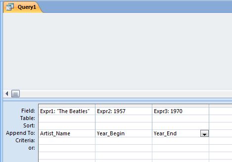 Figure 2.3: MS_Access query design grid GUI showing the layout that will result in appending one record to the database table. Note that an MS-Access Append query is actually translated into an SQL Insert query.
 - Click the Run button to execute this query. Answer Yes when asked whether you really want to append the record to the table.
- Open the Artists table, and confirm that a record for The Beatles exists.
At this point, you may be wondering why we used an Append query when I said we'd use an Insert query. - Go back to the design view window of your query, select View > SQL View, and note that what Access calls an Append query in its GUI is actually an INSERT query when translated to SQL:
INSERT INTO Artists ( Artist_Name, Year_Begin, Year_End )
SELECT "The Beatles" AS Expr1, 1957 AS Expr2, 1970 AS Expr3;
Check the Artists table to verify the addition of the new record. If your Artists table is still open, in the Home ribbon you can select Refresh then Refresh All.
If you're wondering why we bothered to write this query when we could have just entered the data directly into the table, you're right. That would be a waste of time. However, such statements are critical in scenarios in which records need to be added to tables programmatically. For example, if you've ever created a new account through some websites like amazon.com, it is likely that your form entries were committed to the site's database using an INSERT query like this one.
It is important to note that the syntax generated by the Access GUI does not follow standard SQL. Let's modify this SQL so that it follows the standard (and adds another artist to the table). - Change the query so that it reads as follows:
INSERT INTO Artists ( Artist_Name, Year_Begin, Year_End )
VALUES ( "The Kinks", 1964, 1996 );
- Click the Run button to execute the query.
- Finally, modify the query to add one more artist (and note the removal of the Year_End column and value, since The Who are considered an active band):
INSERT INTO Artists ( Artist_Name, Year_Begin )
VALUES ( "The Who", 1964 );
- Execute the query, then close it without saving.
C. Adding records from another table in bulk
The last method of adding records to a table is perhaps the most common one, the bulk insertion of records that are already in some other digital form. To enable you to see how this method works in Access, I've created a comma-delimited text file of albums released in the 1960s by the three artists above.
- Download the Albums.txt file [10] and save it to your machine.
- In Access, go to External Data > Text File. (Note the other choices available, including Access and Excel.)
- Browse to the text file on your machine and select it.
Note the three options available to you: importing to a new table, appending to an existing table and linking to the external table. The second option would make sense in this situation if the column headings in the text file matched those in the target Access table. They do not, so we will import to a new table and build a query to perform the append. - Confirm that the Import option is selected, and click OK.
- The first panel of the Import Text Wizard prompts you to specify whether your text is Delimited or Fixed Width. Confirm that Delimited is selected, and click Next.
- The next panel should automatically have Comma selected as the delimiter and double quotes as the Text Qualifier (i.e., the character used to enclose text strings). Check the First Row Contains Field Names checkbox, and click Next.
- The next panel makes it possible to override the field names and types. The wizard has correctly identified the field types for all but the Label_ID field. Click on the Label_ID heading, and change its data type to Long Integer. Click Next.
- The next panel provides an opportunity to specify the table's primary key. Options include adding a new AutoNumber field, choosing the key from the existing fields, or assigning no primary key at all. Because this table will be of no use to us after appending its records to the Albums table created earlier, select No primary key, and click Next.
- Finally, the last panel prompts you for the name to give to the table. Enter Albums_temp, and click Finish to complete the import.
- This is a one-time import process, so simply click Close when asked if you want to save the import steps.
- Double-click on Albums_temp to open it in datasheet mode, and confirm that the data imported correctly. You're now ready to build a query that will append the records from Albums_temp to Albums.
Note:
The Albums.txt text file you just imported was written assuming that the records in the Labels table are stored with Label_ID values as specified in the figure in Part A and Artist_ID values of 1 for The Beatles, 2 for The Kinks and 3 for The Who. If your tables don't have these ID values (e.g., if you ran into a problem with one of the inserts into the Artists table and had to add that artist again), you should modify the ID values in the Albums_temp table so that they match up with the ID values in your Labels and Artists tables before building the Append query in the steps below.
- Click Create > Query Design to begin building the query.
- Add the Albums_temp table to the query GUI. Do not add the Albums table. Close the Show Table dialog.
- As before, click the Append button to change the query type. You may have to go back to the Design ribbon.
- Select Albums as the Append to table, and click OK.
- Double-click on each of the fields in the Albums_temp table so that they appear in the design grid. Note that the Artist_ID and Label_ID fields are automatically paired up with the fields having the same name in the Albums table. The title and release year fields have different names, so you will have to match those fields up manually.
- In the Append To cell, select Title under the Album_Title field and Release_Year under the Released field.
If we wanted to append a subset of records from Albums_temp, we could add a WHERE clause to the query. We want to append all the records, so our query is done. - Execute the query, and confirm that the Albums table is now populated with 10 records.
- Close the query without saving. You would consider saving it if you found yourself performing this sort of append frequently.
If you were wondering why we didn't just import the text file and use the table produced by the import, that's a good observation. In this particular scenario, that would have been less work. However, the process we just followed is a common workflow, particularly when you are looking to append new records to a table that is already populated with other records. In that scenario, this methodology would be more clearly appropriate.
Updating Existing Records
Updating Existing Records
As with adding records, updating existing records can be done both manually through the GUI and programmatically with SQL. The manual method simply requires navigating to the correct record (sorting the table can often help with this step) and replacing the old value(s) with new one(s).
SQL UPDATE statements are used in a couple of different scenarios. The first is when you have bulk edits to make to a table. For example, let's say you wanted to add a region field to a states table. You might add the field through the table design GUI, then execute a series of UPDATE queries to populate the new region field. The logic of the queries would take the form, "Update the region field to X for the states in this list Y." We'll perform a bulk update like this in a moment.
The other common usage for the UPDATE statement goes back to the website account scenario. Let's say, you've moved and need to provide the company with your new address. Upon clicking the Submit button, a script will generate and execute an UPDATE query on your record in the table.
A. Performing an UPDATE query
After working with your album database for a while, you notice that you're constantly using string concatenation to add the word "Records" to the names of the companies in the Labels table. You decide that the benefit of adding that text to the label names outweighs the drawback of storing that text redundantly.
- Select Create > Query Design.
- Add the Labels table to the query design GUI, and close the Show Tables dialog.
- In the Query Type section of the Design ribbon, change the query type from Select to Update. Note that the Show and Sort rows in the design grid disappear (this query type doesn't show any results) and an Update To row takes their place.
- Double-click on the Label_Name field to add it to the design grid.
- In the Update To cell, enter the following expression (be sure to include the space before the word Records):
[Labels]![Label_Name] & " Records"
If you needed to, you could specify selection criteria to limit the update to a subset of records. For example, following on the state-region example mentioned above, you might update the region field to "New England" using a WHERE condition of:
WHERE state IN ('CT','MA','ME','NH','RI','VT').
In this case, we want to perform this update on all records, so our query is done. - Execute the query and open, or refresh, the Labels table to confirm that it worked.
- Return to the query and select View > SQL View to see the SQL statement that you created through the GUI:
UPDATE Labels SET Labels.Label_Name = [Labels]![Label_Name] & " Records";
As discussed earlier when we were dealing with SELECT queries, the brackets and exclamation point do not follow the SQL standard. You could also omit the parent table in the field specification if there is no chance of duplicate field names in your query. Thus, the following syntax would also work and be closer to standard SQL:
UPDATE Labels SET Label_Name = Label_Name & " Records";
Also, as mentioned before, concatenation requires a different syntax depending on the RDBMS. - Close the query without saving.
Deleting Records
Deleting Records
When working in Access, deleting records can be as easy as opening the table, navigating to the desired records, selecting them using the gray selection boxes to the left of the records, and hitting the Delete key on the keyboard. Likewise, it is possible to follow the same methodology to delete records returned by a SELECT query (if it's a one-table query).
However, as with the other query types, it is sometimes necessary to write a query to perform the task. For example, if you've ever canceled a hotel reservation or an order from an online vendor, a DELETE query was probably executed behind the scenes. Let's see how such a query can be built using the Access GUI and examine the resulting SQL.
A. Deleting records
Let's say a revised version of the 1001 albums list is released, and the albums recorded by The Who on the Track Records label have dropped off the list. Knowing that Track Records no longer has albums on the list, you decide to delete it from the Labels table.
- Select Create > Query Design.
- Double-click on Labels to add it to the query design GUI, then close the Show Tables dialog.
- Change the query type to Delete. As with the Update query, the Sort and Show rows disappear from the design grid, replaced by a Delete row.
- Double-click * to add it to the design grid. You should see the keyword From appear in the Delete row of the design grid.
While it's possible to bring down an individual field instead of *, which implies that it might be possible to delete values in a particular field only, that's not really the case. Delete queries are used to delete entire rows meeting certain criteria. If you want to wipe out the values in a field, leaving other field values intact, you should use an Update query. - Double-click Label_Name to add it to the design grid. You should see the keyword Where appear in the Delete row of the design grid.
- In the Criteria cell, enter "Track Records".
- Execute the query.
- You should be asked to confirm that you really want to delete the 1 record meeting your criteria. Answer Yes to go ahead with the deletion.
- Open the Labels table and verify that the record has been deleted.
- Open the Albums table and note that The Who Sell Out and Tommy have been deleted from that table also. This deletion was carried out because of the Cascade Delete Related Records setting we made earlier. If we had not checked that box, the two albums would be left in the Albums table referring to a record label that does not exist in the Labels table.
- Return to the query, and select View > SQL View. Note the statement produced by the GUI:
DELETE Labels.*, Labels.Label_Name
FROM Labels
WHERE (((Labels.Label_Name)="Track Records"));
Again, this statement could be simplified as follows:DELETE * FROM Labels WHERE Label_Name="Track Records";
- Close the query without saving.
One final note before moving on to the graded assignment. I had you delete the record label from the database because I wanted to show you how to write a DELETE query. However, think about other actions you might have taken instead under that scenario. Depending on the circumstance, it might make more sense to leave that label in the database and delete only the albums (in case the label once again has an album on the list). The upside of deleting the label is that answering a question like, "Which record companies released the albums on the list?" requires dealing only with the Labels table. On the other hand, if the Labels table included companies that had no albums on the list, answering that question would require a more complex query, involving a join between Albums and Labels.
Another response to the revised-list scenario might be to make it possible for the database to store all versions of the list, rather than just its current state. Generally speaking, it's better to err on the side of keeping data versus deleting. Doing so makes your database capable of answering a larger array of questions; it's quite common for database users to come up with questions that could not have been predicted in the initial design. The downside to this decision is that it necessitates changes to the database design. What changes would be required in this scenario?
Project 2: Designing a Relational Database
Project 2: Designing a Relational Database
This lesson focused on concepts involved in the design of a relational database. To demonstrate your understanding of these concepts, you'll now complete an exercise in database design. Here is the scenario; you work for a UFO investigation organization that has collected a lot of information related to sightings, and you've been tasked with designing a database that will be used as the back end for a website. The information to be stored in the database includes the following:
- sighting date/time
- object shape (saucer, cigar, etc.)
- sighting coordinates (latitude, longitude)
- witness name, phone # and email address
- textual descriptions of the sighting
In addition to this basic information, the organization has many digital files that must be made available through the website:
- photos
- videos
- drawings
- audio (interviews with witnesses)
While most RDBMSs make it possible to store such data in the form of BLOBs (Binary Large OBjects), doing so can be tricky. An alternative approach is to store the names of the files and use front-end application logic to present the file data appropriately.
If you have access to software that can be used to produce an entity-relationship diagram of your proposed database structure, feel free to use it. However, hand-drawn and scanned diagrams are perfectly acceptable as well. If you don't have access to a scanner at home or work, try your local library or FedEx Office store.
As part of your submission, please include notations of the key fields (primary and foreign), the relationships and cardinality between tables, and a short narrative that explains the thinking that went into your design.
Deliverables
This project is one week in length. Please refer to the Canvas Calendar for the due date.
- Upload your ER diagram and narrative to the Project 2 Dropbox, 100 of 100 points.
- Complete the Lesson 2 quiz.
Lesson 3: Building a Postgres/PostGIS Database
Overview
Overview
Now that you have a solid handle on the basics of relational database design and query writing, we're ready to dive into spatial database technology. Over the next two lessons, we'll experiment with the open-source RDBMS PostgreSQL (pronounced pōst-grɛs kyü'-ɛl ) and its spatial extension PostGIS (pronounced pōst-jis). This software combination is quite popular for those looking for an alternative to vendor solutions that are often more costly than their organization can afford.
Unlike MS-Access, which is intended for relatively small projects, Postgres is a full-fledged enterprise RDBMS more akin to the leading vendor products (e.g., Oracle and SQL Server). Though there are certainly differences between Postgres and Access, you should find that the concepts you learned earlier in the course will transfer over to this new environment.
After orienting you to working with Postgres, we'll get into the spatial functionality provided by PostGIS.
Objectives
At the successful completion of this lesson, students should be able to:
- create a new database schema in Postgres;
- use the Postgres shapefile loader plugin to import data in Esri's shapefile format;
- write and execute queries in Postgres;
- describe the spatial data types built into PostGIS;
- translate features in textual format into PostGIS geometries;
- imagine scenarios for storing multiple geometry columns or multiple geometry types in the same PostGIS table;
- view PostGIS tables as layers in QGIS;
- use QGIS to conduct basic GIS operations (such as creating a simple map).
Questions?
If you have any questions now or at any point during this week, please feel free to post them to the Lesson 3 Discussion Forum.
Checklist
Checklist
Lesson 3 is one week in length. See the Canvas Calendar for specific due dates. To finish this lesson, you must complete the activities listed below:
- If you haven't already done so, please download and install Postgres, PostGIS, and QGIS (an open-source desktop GIS package we'll use to view our PostGIS data):
-
Download and install Postgres 16.x [11], accepting all of the default settings - Go with the 64-bit version unless your computer will not support it.
When running the installation, you will need to have access to the Internet.- After Postgres is installed, you'll be asked if you want to launch the Stack Builder, a separate package that allows for the installation of add-ons to Postgres. Check the box for Stack Builder may be used... and in the next window, choose PostgreSQL 16.x on Port 5432 as the installation you are installing software for.
- Under the category of Spatial Extensions, choose the PostGIS 3.4 Bundle... Installing this add-on will enable you to execute the spatial queries covered in Lessons 3-4.
- Make your way through the installation, accepting the defaults. When the Choose Components dialog appears, check the Create spatial database box.
- For the Database Connection, leave the User Name set to postgres and Port set to 5432. Set the Password to postgres, same as the User Name, making it easy to remember.
- For the Database Name, leave it set to the default of postgis_34_sample.
- Installing PostGIS if Postgres is already installed - A separate installer file is available for the version that accompanies the 64-bit version of Postgres. If for some reason you do not use the Stack Builder noted above, you can use this installer. Locating the installer [12] at the postgis.net site is a bit tricky, so here is a direct link.
- Install QGIS [13] - click the QDownload QGIS 3.34 link under the Windows heading, and run the downloaded setup file to install QGIS.
-
- In addition to these software downloads, please also download and unzip the data needed for Lesson 3 [14].
- Work through Lesson 3.
- Complete Project 3, and upload its deliverables to the Project 3 Dropbox.
- Complete the Lesson 3 Quiz.
Getting Started with PostGIS
Getting Started with PostGIS
In this first part of the lesson, you'll get an introduction to Postgres's graphical interface called pgAdmin. You'll also import a shapefile, load data from a text file, and see how queries are performed in pgAdmin.
A. Create a new schema
- Open pgAdmin 4. The application should open with a pane on the left side of the window labeled Browser. Within the Browser, you should see a tree with Servers at the top. Beneath Servers, you should see a Postgres 16 server.
- Double-click on that server to open a connection to it. You will be logging in with the default user name of postgres.
Enter the password you defined earlier for the postgres account when you installed the software. You should now see 3 nodes beneath the localhost server: Databases, Login/Group Roles, and Tablespaces. - Expand the Databases list. You should see at least one "starter" database: postgres. It was created when you installed Postgres.
We want to create a new database that is specific to our desire to use the PostGIS functionality. - Right-click on the Databases list, and choose Create > Database.
- In the Create - Database dialog, set the Database to Lesson3db, and from the Owner list, select the postgres user name.
Hit Save. - Now, click on the Lesson3db database to expand its list of contents.
Right-click on Extensions, and select Create > Extension. - In the Create Extension dialog under the General tab, set the Name to postgis.
In the same dialog, select the Definition tab, and set the Version to 3.4.x.
(The settings you just established are reflected under the SQL tab.)
Click Save to dismiss the Create Extension dialog.
We will next concern ourselves with schemas. In Postgres, schemas are the containers for a set of related tables. Generally speaking when you begin a new project, you'll want to create a new schema. - Expand the Schemas list. At this point, you should see only one schema: public. We'll have a look at the public schema soon; but for now, let's create a new schema. This schema will store data for the United States that we will use in the next two lessons.
- Right-click on Schemas, and select Create > Schema.
- In the Create Schema dialog, specify a name of usa.
- Set the Owner of the schema to postgres.
- Click Save to create the schema.
B. Load data from a shapefile
A common workflow for PostGIS users is to convert their data from Esri shapefile format to PostGIS tables. Fortunately, some PostGIS developers have created a Shapefile Import/Export Manager that makes this conversion easy. In prior versions of pgAdmin, the shapefile importer was accessible as a plug-in. In pgAdmin 4, it must be run as a separate application.
- In Windows File Explorer, browse to the following folder:
C:\Program Files\PostgreSQL\16\bin\postgisgui - Run the executable shp2pgsql-gui.exe.
Note:
If you encounter an error that the file "libintl-9.dll is missing," the easiest fix for this problem is to navigate up to the bin folder where libintl-9.dll is found, copy it, and paste it into the postgisgui folder.
Since we will be using this executable several times, I suggest that you make a desktop shortcut for it. - At the top of the application window, click the View connection details button.
- Confirm that the PostGIS Connection parameters are set as follows:
Username: postgres
Password: <the password you set when installing the software>
Server Host: localhost (port 5432)
Database: Lesson3db - In the middle of the dialog, click the Add File button and navigate to the location of your Lesson 3 data.
- Select States.shp and click Open.
- In the Import List section of the dialog (above the Add File button) supply the following settings by clicking on the current values under each heading:
Schema: usa
Table: states
Geo Column: geom
SRID: 4269 (After setting this last value, be sure to click away from the row of specifications or hit Enter; otherwise, the last value changed may revert to its original value of 0.)
Before performing the import, let's spend a moment discussing the SRID (Spatial Reference IDentification) setting. This ID is set to 0 by default, a value that indicates the spatial reference of the shapefile is unknown. As with other GIS applications, defining a dataset's spatial reference is critical in enabling most of the functionality we typically need. We'll talk more about SRIDs later. For now, it's sufficient to know that 4269 is the ID associated with the decimal degree/NAD83 coordinate system used by the Lesson 3 data. - Click Import. After just a moment, the Log Window area of the dialog should report that the import process has been completed.
- Close the Import/Export Manager application by clicking the X button in the upper right of the dialog or on the Cancel button.
- Back in pgAdmin, expand the object list associated with the usa schema.
- Click on Tables. You should now see the newly imported states table.
Note:
It's sometimes necessary to refresh the GUI after creating new objects like this. This can be done by right-clicking on the schema or Tables node in the Browser and selecting Refresh (or hitting F5 on the keyboard).
- Right-click on the states table and select View/Edit Data > First 100 Rows. Note the other options in this context menu, which are rather straightforward to understand.
While looking at the table, note that the column headers include not just the names of the columns but also their data types. The gid column is an auto-incrementing integer column that was added by the importer. The presence of [PK] in its header indicates that it was also designated as the table's primary key.
Also note that the geom column header contains a "map" icon. Clicking it allows you to see the table's geometries on a simple map.
- Repeat these steps to import the us_cities shapefile. Truncate its name to just cities. Also note for future reference that although we didn't do so here, you may import multiple shapefiles at a time.
- Click Cancel to close the Shapefile Import/Export Manager.
C. Create a new table
Loading data from a comma-delimited text file is a common workflow for database developers. Let's see how this can be done in Postgres by loading some state demographic info from the 2010 Census. We'll begin by creating a new blank table.
- To create a new table, right-click on Tables under the usa schema and select Create > Table.
- Under the General tab, set the table's Name to census2010 and the Owner to postgres.
- Under the Columns tab, click the + button. You should see an entry appear for setting the new column's properties.
- Set the column's Name to state, its Data type to character varying and its Length to 50. Finally, switch the toggle in the under the Primary key? heading to on.
- Repeat the last two steps to add a column with the Name total and Data type of integer. The length property need not be set for the integer type and the column should not be defined as the primary key.
- Add the following additional columns to the table, all as integer data type.
Note:
Instead of having to expand the Data Type pick list, you can start typing the word integer, and the slot will let you autofill with choices. After you type inte, you can pick "integer." Be sure to add the columns in this order, otherwise the data load will not work properly.
Table 3.1: Additional Integer columns to be added to your usa.census2010 table.male female white black amind asian hawaiian other mixed - Click Save to finish creating the table.
D. Load data using the COPY command
Before executing the command that will import the data into the table, let's have a look at the data file in a plain text editor and also note its location.
- In Windows Explorer right-click on the census2010.csv file and select Open With > Notepad. Note that the values in the file are comma delimited and that the file includes a header row. Close the file when finished examining it.
- Determine the full path name of the location of your census2010.csv file. The format that you will need to use is as follows with the drive letter followed by the folder names and finally the file name. Something like C:\Users\Smith\Documents\Lesson3data\census2010.csv
- In pgAdmin, select Tools > Query Tool. The Query Tool dialog is built such that the SQL code is entered in the top and the query's output appears in the bottom.
- Enter the following command, changing the path to reflect the census2010.csv file location on your machine.
COPY usa.census2010 FROM 'C:\PSU\Geog868\Lesson3data\census2010.csv'
WITH (FORMAT csv, HEADER True);
Let's look for a moment at the options set in the WITH clause. If our input file were tab-delimited, we would use a FORMAT setting of text rather than csv. We set the HEADER option to True since our file contains a header row. A number of other options are available and can be found on the COPY command's page [16] in the documentation. One option you may need to set is DELIMITER. This defaults to the comma for csv files and to tab for text files. If your file uses another delimiter, such as the pipe character (|), you can indicate that using the DELIMITER option. Another option to note is QUOTE. Delimited text files often have text strings embedded within quotation marks. This is done to explicitly differentiate those values from numeric or Boolean values. Typically this quoting is done with the double-quote character. When Postgres copies the data from the text file to your table, it omits the quoting character. For example, "SMITH" in the text file becomes SMITH in the table. By default, Postgres assumes that such quoting will be done with the double quote. However, if your file's strings are instead denoted by a single quote or some other character, you can specify that by setting the QUOTE option to the appropriate character.Note:
If you encounter a "permission denied" error, it means the "postgres" database login doesn't have permission to read the csv file where it is currently located. Try copying it to a sub-directory belonging to the "Public" user (e.g., 'C:\Users\Public\Public Documents') or to a location that has no permission restrictions (e.g., 'C:\temp'). You could also reset the permissions on the folder that stores the CSV file as outlined in this stackoverflow thread [15].
The COPY command attempts to insert values from the first column of the input file into the first column of the table, values from the second column of the input file into the second column of the table, etc. The HEADER option simply tells Postgres to skip the first line; it does not tell it to read the column headers and intelligently match the columns of the input file to the columns of the table. If your table happens to have more columns than the input file, and/or the columns are in a different order, you can deal with this by supplying to the COPY command a list of column names that matches the input file after the table name. For example:COPY usa.census2010 (state, total, male....) FROM ....
- Execute the command by clicking the Execute button ("Play" icon) just above the SQL code box. You should receive a message that the query returned successfully with 52 rows affected.
- Confirm that the data loaded properly using the method you used for the states table.
E. Write queries in pgAdmin
- Click on Tools > Query Tool again to open a new query tab.
- In the SQL box, enter the following query to identify the states where most of the population uses the term 'Soda' when referring to soft drinks:
SELECT name, sub_region
FROM states
WHERE sub_region = 'Soda';
- Run the query by clicking the Execute button on the toolbar. You should receive an error message that the relation "states" does not exist.
- The reason for this error has to do with pgAdmin's search path. Among other things, the search path determines which schema(s) will be scanned when tables are specified using unqualified names (e.g., like we just did with "states"). There are two solutions to this problem. The first is to qualify all table names with their parent schema. For example:
SELECT name, sub_region
FROM usa.states
WHERE sub_region = 'Soda';
The second solution is to reset pgAdmin's search path so that the schema you're using is part of that path. By default, pgAdmin searches only the public schema. We will take this second approach since it allows us to omit the schema qualifier. - So, highlight the text of your query and cut it out of the editor window. We'll be pasting it back in momentarily.
- Enter the following statement into the SQL Editor:
SET search_path TO usa, public;
- Run this query by clicking the Execute button. You should receive a message that the query returned successfully, though you should expect no tabular output from a query like this. pgAdmin will now look for unqualified tables first in the usa schema, then in the public schema. We include the public schema because the search path is used not just for searching for tables but also for functions. When we move on to spatial queries, we'll need to have access to some of the functions available in the public schema.
If you are curious, you can run the following query to find out what the search path is set to.SHOW search_path;
- You can now retry the query that you cut out. You should see a list of 17 states in the Output pane at the bottom of the window.
Note:
You may still be receiving an error if you left the table's name set to States rather than states during the import process; pgAdmin converts all table/column names to lower-case prior to execution by default. Thus, even if your FROM clause reads "FROM States", it will be evaluated as "FROM states". And if your table is named States, pgAdmin won't find a matching table. To override this case conversion, you can put the table/column name in double quotes like this:
SELECT name, sub_region
FROM "States"
WHERE sub_region = 'Soda';
To avoid having to qualify your table/column names in this way, it's best to use lower case in your naming.
- While on the subject of case, you may have noticed that my examples place all SQL keywords in upper case and table/column names in lower case. This is a convention that is followed by many SQL developers because it makes it easy to tell at a glance which parts of the statement are SQL keywords and which are schema elements. This is just a convention, not a requirement, so you should feel free to deviate from it if you prefer. For example, this query will produce the same results:
select name, sub_region
from states
where sub_region = 'Soda';
Now that you have a feel for how Postgres works, go on to the next page to practice writing queries in pgAdmin.
Query-Writing Practice Exercises
Query-Writing Practice Exercises
To help you get oriented to writing SQL queries on the pgAdmin command line, try your hand at the following exercises. Recall that the 2008 population data, soft drink data, and geometries are in the states table, and that the 2010 data are in the census2010 table.
- Select the states with a 2008 population over 10 million.
- Select the state capitals.
- Select the states whose names begin with the word "New".
- Select the cities whose names contain the letter "z".
- Sort the states by their 2008 population from high to low.
- Sort the states first by soft drink name then by state name.
- Select the states with a 2008 population over 10 million and where the majority of the population refers to soft drinks as pop.
- Select cities in the states of NY, NJ, and PA (using the stateabb column).
- For each state, compute the percentage of the 2010 population that is white. Give this output column an alias of pctwhite. Besides pctwhite, include only the name of the state in the output. Note: the columns involved in this calculation are defined as integers, which means the resulting value will be rounded to the nearest integer (0). To avoid this rounding and obtain the desired percentages, add '::double precision' after the white column in the calculation. This will convert the integer values to double precision values prior to the calculation. It is only necessary to perform this conversion for one of the columns involved in the calculation.
- Sum the 2008 state populations across the soft drink categories (i.e., What is the population of the 'soda' states? Of the 'pop' states? Of the 'coke' states?).
- Bring together data from the states and census2010 tables, outputting the name from the states table, total population from the census2010 table and geom from the states table.
- Calculate the average 2010 male population across the soft drink categories.
Solutions [17] (This link takes you to the bottom of the Lesson.)
Introduction to Spatial Select Queries
Introduction to Spatial Select Queries
What sets spatial databases apart from their non-spatial counterparts is their support for answering geometric and topological questions. Let's have a look at some simple examples to demonstrate. We'll continue working with the states table we created in the last section.
- Return to the Query dialog in pgAdmin and execute the following query:
SELECT name, ST_Centroid(geom) AS centroid
FROM states
WHERE sub_region = 'Soda';
The obvious difference between this and our earlier queries is that it calls upon a function called ST_Centroid(). Like the functions we worked with in Lesson 1, the ST_Centroid() function accepts inputs and returns outputs. Here, we supply the geom column as an input to the function, and it returns the geometric centers of the shapes stored in that column.
You've probably noticed that the output from ST_Centroid() is not human friendly. It contains the coordinates of a point in the coordinate system of the input column, but expressed in hexadecimal notation [18]. To display the coordinate values in a more readable form, we can nest the call to the ST_Centroid() function within a call to a function named ST_AsText(). - Modify the query as follows, then execute:
SELECT name, ST_AsText(ST_Centroid(geom)) AS centroid
FROM states
WHERE sub_region = 'Soda';
In this version of the query, the hexadecimal value returned by ST_Centroid() is immediately passed to the ST_AsText() function, which returns a value formatted for human consumption (with longitude listed first, latitude second).
Now, let's try retrieving the areas of the states using ST_Area(). - Modify the query as follows, then execute:
SELECT name, ST_AsText(ST_Centroid(geom)) AS centroid, ST_Area(geom) AS area
FROM states
WHERE sub_region = 'Soda';
In the area column, take note of the values returned by ST_Area(). They are in the units of the input geometry, squared. Recall that the Lesson 3 shapefiles are in latitude/longitude coordinates, which means the area values we're seeing are in square degrees. Hopefully, you recognize that this is a poor way to compute area, since a square degree represents a different area depending on the part of the globe you're dealing with. The ST_Transform() function exists exactly for situations like this. It takes a geometry (in whatever spatial reference) as input and re-projects it into some other spatial reference. - Modify the query as follows, then execute:
SELECT name, ST_AsText(ST_Centroid(geom)) AS centroid, ST_Area(ST_Transform(geom,2163)) AS area
FROM states
WHERE sub_region = 'Soda';
Take note of the values now displayed in the area column. In this version of the query, the ST_Transform() function is first used to re-project the geometry into the spatial reference 2163 before ST_Area() is called. That spatial reference is an equal-area projection in meters that is suitable for the continental U.S. Don't worry, we'll discuss how you'd find that information later in this lesson.
Note: ST_Transform() re-projects input geometries in memory only, the input geometries stored in the table remain in the same spatial reference they had before.
We'll spend much more time discussing the spatial functions that are available in PostGIS later. Right now, let's go over the geometry types that are supported.
PostGIS Geometry Types
PostGIS Geometry Types
In the last section, we worked with a table – usa.states – containing geometries of the type POLYGON. The other basic geometry types are POINT and LINESTRING. As we'll see momentarily, there are numerous other geometry types available in PostGIS that allow for the storage of multipart shapes, 3-dimensional shapes, and shapes that have a measure (or M value) associated with its vertices. If keeping all of the various types straight becomes difficult, it may help to remember that the simple geometries we deal with most often are POINT, LINESTRING, and POLYGON.
To demonstrate some of the concepts in this section, we're going to create a new schema to store points of interest in New York City. Unlike the last schema where we used the Shapefile Import/Export Manager to both create and populate a table at the same time, here we'll carry out those steps separately.
A. Create a new empty spatial table
- In the Browser pane within pgAdmin, right-click on the Schemas node beneath the Lesson3db database and select Create > Schema.
- Set the Name of the schema to nyc_poi and its Owner to postgres, then click Save to create the schema.
- Expand the object listing associated with the nyc_poi schema.
- Right-click on the Tables node, and select Create > Table.
- Set the table's Name to pts and its Owner to postgres.
- Under the Columns tab, click the + button.
- For the new column, set the Name to gid (geometry ID) and the Data type to serial. This data type is roughly equivalent to the AutoNumber type we saw in Access. Define this column as the table's Primary key.
- Repeat the previous step to create a column called name. Set its Data type to character varying and its Length to 50. This column should not be the Primary key.
The last column we want to add to the table is one that will hold the geometries. While it's possible to add a column of type 'point' through the GUI, there are a number of other important settings that should be made when adding a geometry column (such as its spatial reference ID, or SRID). These settings are all handled by a PostGIS maintenance function called AddGeometryColumn(), so that is the route we will take.
- Click Save to dismiss the dialog and create the table. Before adding the geometry column to the table, let's recall the pgAdmin search path. It's not set to include the nyc_poi schema, so let's do that first.
- Reset the search path by executing the following statement in a Query window:
SET search_path TO nyc_poi, public;
- Now add a geometry column called geom to the table by executing this statement. (You can re-use the Query window you already have open for this and subsequent queries.)
SELECT AddGeometryColumn('nyc_poi','pts','geom',4269,'POINT',2);First, let's address the unusual syntax of this statement. You've no doubt grown accustomed to listing column names (or *) in the SELECT clause, but here we're plugging in a function without any columns. We're forced to use this awkward syntax because SQL rules don't allow for invoking functions directly. Function calls must be made in one of the statement types we've encountered so far (SELECT, INSERT, UPDATE, or DELETE). In this situation, a SELECT statement is the most appropriate.
The arguments to the function in this statement are, in order: the schema name, the table name, the name to be given to the geometry column, its spatial reference ID, the type of geometry it will store, and the dimension of the coordinates it will hold.
Before moving on, an explanation of this dimension parameter is in order. In most cases, you're likely to be storing just X and Y coordinates. When that's the case, you should assign a dimension value of 2, as we just did. However, it is also possible that you want to store the elevation (Z value) of the points. In that case, you assign a dimension value of 3. As mentioned above, it is also possible to store some type of measure (M value) with each point (e.g., the time the point was recorded with a GPS unit). In that scenario, you would also assign a dimension value of 3. You would differentiate that XYM type of point from an XYZ point by setting the geometry type to POINTM instead of POINT. Finally, it is possible to store all four values (X, Y, Z and M). In that situation, you would assign a dimension value of 4.
B. Add rows to the spatial table
We're about to add rows to our pts table through a series of INSERT statements. You'll find it much easier to copy and paste these statements rather than typing them manually, if not now, then certainly when we insert polygons later using long strings of coordinates.
- Execute the following statement to insert a row into the pts table.
INSERT INTO pts (name, geom)
VALUES ('Empire State Building', ST_GeomFromText('POINT(-73.985744 40.748549)',4269));
The key point to take away from this statement (no pun intended) is the call to the ST_GeomFromText() function. This function converts a geometry supplied in text format to the hexadecimal form that PostGIS geometries are stored in. The other argument is the spatial reference of the geometry. This argument is required in this case because when we created the geom column using AddGeometryColumn(), it added a constraint that values in that column must be in a particular spatial reference (which we specified as 4269). - Execute the statements below to add a couple more rows to the table. Note that while we've executed single statements thus far in the lesson, you are also allowed to execute multiple statements in succession.
INSERT INTO pts (name, geom) VALUES ('Statue of Liberty', ST_GeomFromText('POINT(-74.044508 40.689229)',4269)); INSERT INTO pts (name, geom) VALUES ('World Trade Center', ST_GeomFromText('POINT(-74.013371 40.711549)',4269)); - Next, execute the statement below, noting the use of the ST_MakePoint() function nested within the ST_SetSRID() function. In many situations, PostGIS offers multiple ways to accomplish the same task. In this case, the inner function (ST_MakePoint) is executed first, creating a POINT geometry, which then serves as an input to the outer function (ST_SetSRID), which sets the SRID of the POINT.
INSERT INTO pts (name, geom) VALUES ('Grand Central Station', ST_SetSRID(ST_MakePoint(-73.976522, 40.7528),4269)); - Finally, add two more rows using the statement below. Note that in this step you're adding multiple rows using a single statement.
INSERT INTO pts (name, geom) VALUES ('Radio City Music Hall', ST_GeomFromText('POINT(-73.97988 40.760171)',4269)), ('Madison Square Garden', ST_GeomFromText('POINT(-73.993544 40.750541)',4269)); - In the pgAdmin window, right-click on the pts table and select View/Edit Data > All Rows to confirm that the INSERT statements executed properly.
C. Create and populate a table of linestrings
- Repeat the steps (in Part A above) to create a new table within the nyc_poi schema, that will hold NYC line features. Pay particular attention to these differences:
- Give the table a name of lines.
- The table should have the same column definitions, with the exception that the geometry type should be set to LINESTRING rather than POINT.
- No need to set the search path again, as it will already include the nyc_poi schema.
- Execute the following statement to insert 3 new rows into the lines table:
INSERT INTO lines (name, geom)
VALUES ('Holland Tunnel',ST_GeomFromText('LINESTRING(
-74.036486 40.730121,
-74.03125 40.72882,
-74.011123 40.725958)',4269)),
('Lincoln Tunnel',ST_GeomFromText('LINESTRING(
-74.019921 40.767119,
-74.002841 40.759773)',4269)),
('Brooklyn Bridge',ST_GeomFromText('LINESTRING(
-73.99945 40.708231,
-73.9937 40.703676)',4269));
Note that I've split this statement across several lines to improve its readability, not for any syntax reasons. You should feel welcome to format your statements however you see fit.
As you can see, the syntax for constructing linestrings is similar to that of points. The difference is that instead of supplying just one X/Y (lon/lat in this case) pair, you supply however many pairs are needed to delineate the feature, with the pairs being connected sequentially by straight line segments. The longitude (X) value comes first and is separated from the latitude (Y) by a space. The lon/lat pairs are in turn separated by commas. For simplicity's sake, I gave you the coordinates of some very simple straight lines. In a real-world situation, you would likely need many lon/lat pairs for each line feature, the number depending on the curviness of the feature.
D. Create and populate a table of polygons
- Repeat the steps (in Part A) to create a new table within the nyc_poi schema, with the following exceptions:
- Give the table a name of polys.
- Set the geometry type of the geom column to POLYGON rather than LINESTRING.
- Execute the following statement to add a row to your polys table:
INSERT INTO polys (name, geom)
VALUES ('Central Park',ST_GeomFromText('POLYGON((
-73.973057 40.764356,
-73.981898 40.768094,
-73.958209 40.800621,
-73.949282 40.796853,
-73.973057 40.764356))',4269));
While the syntax for constructing a polygon looks very similar to that of a linestring, there are two important differences:- The first X/Y (lon/lat) pair should be the same as the last (to close the polygon).
- Note that the coordinate list is enclosed in an additional set of parentheses. This set of parentheses is required because polygons are actually composed of potentially multiple rings. Every polygon has a ring that defines its exterior. Some polygons also have additional rings that define holes in the interior. When constructing a polygon with holes, the exterior ring is supplied first, followed by the interior rings. Each ring is enclosed in a set of parentheses, and the rings are separated by commas.
To see an example, let's add Central Park again, this time cutting out the large reservoir near its center.
- First, let's remove the original Central Park row. In pgAdmin, right-click on the polys table and select Truncate > Truncate. Note that this deletes all rows from the table.
- Add Central Park (minus the reservoir) back into the table using this statement:
INSERT INTO polys (name, geom)
VALUES ('Central Park',ST_GeomFromText('POLYGON((
-73.973057 40.764356,
-73.981898 40.768094,
-73.958209 40.800621,
-73.949282 40.796853,
-73.973057 40.764356),
(-73.966681 40.785221,
-73.966058 40.787674,
-73.965586 40.788064,
-73.9649 40.788291,
-73.963913 40.788194,
-73.963333 40.788291,
-73.962539 40.788259,
-73.962153 40.788389,
-73.96181 40.788714,
-73.961359 40.788909,
-73.960887 40.788925,
-73.959986 40.788649,
-73.959492 40.788649,
-73.958913 40.78873,
-73.958269 40.788974,
-73.957797 40.788844,
-73.957497 40.788568,
-73.957497 40.788259,
-73.957776 40.787739,
-73.95784 40.787057,
-73.957819 40.786569,
-73.960801 40.782394,
-73.961145 40.78215,
-73.961638 40.782036,
-73.962518 40.782199,
-73.963076 40.78267,
-73.963677 40.783661,
-73.965694 40.784457,
-73.966681 40.785221)
)',4269));
E. 3- and 4-dimensional geometries
Earlier in this section, we discussed 3-dimensional (XYZ and XYM) and 4-dimensional (XYZM) geometries in the context of properly specifying the dimension argument to the AddGeometryColumn() function. We won't be doing so in this course, but let's look for a moment at the syntax used for creating these geometries.
To define a column that can store M values as part of the geometry, use the POINTM, LINESTRINGM, and POLYGONM data types. When specifying objects of these types, the M value should appear last. For example, an M value of 9999 is attached to each coordinate in these features from our nyc_poi schema:
POINTM(-73.985744 40.748549 9999)

LINESTRINGM(-74.019921 40.767119 9999, -74.002841 40.759773 9999)

POLYGONM((-73.973057 40.764356 9999,
-73.981898 40.768094 9999,
-73.958209 40.800621 9999,
-73.949282 40.796853 9999,
-73.973057 40.764356 9999)
Perhaps the most common usage of M coordinates is in linear referencing (e.g., to store the distance from the start of a road, power line, pipeline, etc.). This Wikipedia article on Linear Referencing [19] provides a good starting point if you're interested in learning more.
To define a column capable of storing Z values along with X and Y, use the "plain" POINT, LINESTRING and POLYGON data types rather than their "M" counterparts. The syntax for specifying an XYZ coordinate is the same as that for an XYM coordinate. The "plain" data type name tells PostGIS that the third coordinate is a Z value rather than an M value. For example, we could include sea level elevation in the coordinates for the Empire State Building (in feet):
POINT(-73.985744 40.748549 190).
Finally, in the event you want to store both Z and M values, again use the "plain" POINT, LINESTRING and POLYGON data types. The Z value should be listed third and the M value last. For example:
POINT(-73.985744 40.748549 190 9999)
F. Multipart geometries
PostGIS provides support for features with multiple parts through the MULTIPOINT, MULTILINESTRING, and MULTIPOLYGON data types. A classic example of multipart geometry is the state of Hawaii, which is composed of multiple disconnected islands. The syntax for specifying a MULTIPOLYGON builds upon the rules for a regular POLYGON; the parts are separated by commas and an additional set of parentheses is used to enclose the full coordinate list. The footprints of the World Trade Center Towers 1 and 2 (now fountains in the 9/11 Memorial) can be represented as a single multipart polygon as follows:
MULTIPOLYGON(((-74.013751 40.711976, -74.01344 40.712439,
-74.012834 40.712191,
-74.013145 40.711732,
-74.013751 40.711976)),
((-74.013622 40.710772,
-74.013311 40.711236,
-74.012699 40.710992,
-74.013021 40.710532,
-74.013622 40.710772)))
This basic example shows the syntax for storing just X and Y coordinates. Keep in mind that Z values and M values are also supported for multipart geometries. As you might guess, the "MULTI" data types have "M" counterparts too: MULTIPOINTM, MULTILINESTRINGM and MULTIPOLYGONM.
G. Mixing geometries
The tables we've created so far reflect a bias toward Esri-centric design with each table storing a single column of homogeneous geometries (i.e. all points, or all lines, or all polygons, but not a mix). However, PostGIS supports two design approaches that are good to keep in mind when putting together a database:
- It is possible to store multiple geometry columns in a table. This capability could be used to store data in two or more different spatial reference systems. Though one should do so under limited circumstances, given the existence of the ST_Transform() function and the additional maintenance such a design would require.
- It is possible to store multiple geometry types in a single column. This capability can simplify schema design and certain types of queries, though there are drawbacks to this approach, such as the fact that some third-party tools can't deal with mixed-geometry tables.
Let's see how this heterogeneous column approach can be used to store all of our nyc_poi data in the same table.
- Repeat the steps (in Part A) to create a new table within the nyc_poi schema. Pay particular attention to these differences:
- Give the table a name of mixed.
- The table should have the same column definitions, with the exception that the geometry type should be set to GEOMETRY.
- Add the same features to this new table by executing the following statement:
INSERT INTO mixed (name, geom) VALUES ('Empire State Building', ST_GeomFromText('POINT(-73.985744 40.748549)',4269)), ('Statue of Liberty', ST_GeomFromText('POINT(-74.044508 40.689229)',4269)), ('World Trade Center', ST_GeomFromText('POINT(-74.013371 40.711549)',4269)), ('Radio City Music Hall', ST_GeomFromText('POINT(-73.97988 40.760171)',4269)), ('Madison Square Garden', ST_GeomFromText('POINT(-73.993544 40.750541)',4269)), ('Holland Tunnel',ST_GeomFromText('LINESTRING( -74.036486 40.730121, -74.03125 40.72882, -74.011123 40.725958)',4269)), ('Lincoln Tunnel',ST_GeomFromText('LINESTRING( -74.019921 40.767119, -74.002841 40.759773)',4269)), ('Brooklyn Bridge',ST_GeomFromText('LINESTRING( -73.99945 40.708231, -73.9937 40.703676)',4269)), ('Central Park',ST_GeomFromText('POLYGON(( -73.973057 40.764356, -73.981898 40.768094, -73.958209 40.800621, -73.949282 40.796853, -73.973057 40.764356))',4269)); - In the pgAdmin window right-click on the mixed table and select View/Edit Data > All Rows to confirm that the INSERT statement executed properly.
At some point in this lesson, you probably thought to yourself, "This is fine, but what if I want to see the geometries?" Well, you can get a quick look at the geometries returned by a query in pgAdmin by clicking on the "eye" icon that appears on the right side of the geometry column header. But you'll likely want to go beyond this, for example, to utilize your geometries in the context of other data layers. That is the focus of the next part of the lesson, where we will use the third-party application Quantum GIS (QGIS) to view our PostGIS data.
Viewing Data in QGIS
Quantum GIS (QGIS, pronounced kyü'-jis) is a free and open-source desktop GIS package analogous to Esri's ArcMap/ArcGIS Pro. Because of its support for viewing PostGIS data and strong cartographic capabilities, QGIS and PostGIS are often found paired together. (OpenJUMP is another desktop application often used in combination with PostGIS, though its strengths are in spatial querying and geoprocessing.)
A. Add PostGIS data to QGIS
Let's see how QGIS can be used to view the tables we created and populated in the previous section.
- Open QGIS. It'll be the QGIS Desktop 3.x choice from the QGIS folder in your Start menu.
Double-click the New Empty Project option under Project Templates.
The basic elements of the application GUI are similar to ArcMap/ArcGIS Pro's. The Layers panel in the lower left of the window lists the project layers and their symbology, while the much wider pane to the right displays the layer features themselves. Across the top of the window is a set of toolbars that can be moved to custom positions by the user.
Above the Layers panel is the Browser panel, which provides an interface for browsing data sources. Moving from top to bottom:- Favorites - for enabling easy access to frequently used folders on your file system
- Spatial Bookmarks - for saving map extents that you'd like to return to later
- Home - for accessing data located within your folder in C:\Users
- C:\ - for accessing data anywhere on your hard drive
The folder navigation items above can be used to add file-based datasets to your project, such as Esri shapefiles or CSV files.
- GeoPackage - for data in an interchange format from the Open Geospatial Consortium (OGC)
- SpatiaLite - for data stored in a SpatiaLite database [20] (another free and open-source spatial database extension similar to PostGIS, built to add spatial functionality to an RDBMS called SQLite [21])
- PostgreSQL - for PostGIS data
- SAP HANA - for data stored in SAP HANA spatial databases
- MS SQL Server - for data stored in Microsoft SQL Server spatial databases
- Oracle - for data stored in Oracle Spatial databases
- WMS/WMTS - for data streamed via a Web Mapping Service or Web Map Tile Service
- Vector Tiles - for adding vector-tiled basemaps
- XYZ Tiles - for adding raster-tiled basemaps
- WCS - for data streamed via a Web Coverage Service
- WFS - for data streamed via a Web Feature Service
- ArcGIS REST Servers - for map service or feature service data published via an ArcGIS Server instance
- Right-click on the PostgreSQL entry and select New Connection.
- In the Create a New PostGIS connection dialog supply the following information. (See Figure 3.1, below.)
- Name: Lesson3
- Service - (leave blank)
- Host: localhost
- Port: 5432
- Database: Lesson3db
- SSL mode: disable
- Session role - (leave blank)
Supplying your authentication information can be done in a simple, but insecure way or a more secure way that requires a bit more effort. The simple way is to enter your authentication parameters under the Basic tab. They will be stored as part of the QGIS project file (.qgs), assuming you save your work, where they could be read fairly easily. The more secure way is to create a configuration under the Configurations tab. To do this, you would click the + icon, and, in the resulting dialog, give your configuration a name (e.g., Local Server), specify the URL of the PostGIS instance (or leave blank if using the one on your own machine), then supply the authentication parameters. If going this route, your credentials are stored in encrypted form in a QGIS authentication database on your machine.
You're welcome to choose either method, though for the purposes of this class, it should be fine to select the Basic method.
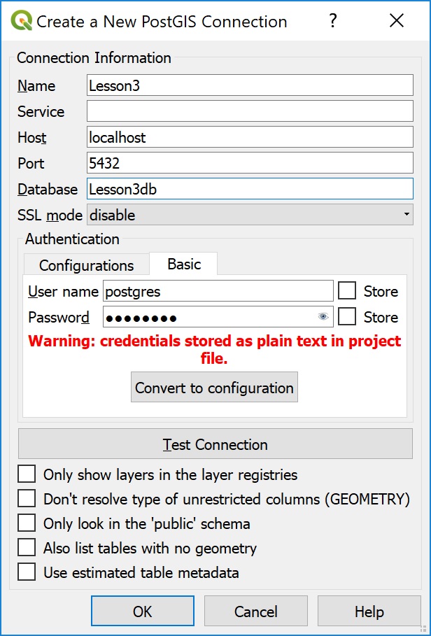
Figure 3.1: The Create a New PostGIS connection dialog, showing the correct information entered.
- You should click the Test Connection button to make sure you have typed things correctly.
- Click OK to create the connection and dismiss the dialog.
Lesson3 should now appear as a PostgreSQL data source. - Now, click the arrow next to the Lesson3 entry to expand the list of schemas made available through that connection.
If an Enter Credentials dialog pops up, just supply the postgres user name and the password you established for it. - Expand the list of layers available in the nyc_poi schema. You should see the pts, lines, and polys tables created early in the last section and also three layers that reference the mixed table created later (one layer for each geometry type). One of the convenient features of QGIS is that it automatically creates separate layers for each geometry type in a multi-geometry table, like our mixed table. The mixed layers can be differentiated by the icons that indicate the geometry type.
- Highlight all 6 nyc_poi datasets and drag them onto the map canvas (or right-click and choose Add Selected Layers to Project). You should see a Select Transformation dialog since the SRID assigned to the geometries in the selected tables (4269, NAD83) is of a different datum than the project's datum (WGS84, from SRID 4326). Click OK to accept the pre-selected NAD83 to WGS84 transformation. You should see your data displayed in the map display area and the layers listed in the Layers Panel on the bottom left of the window.
Now let's take a quick tour of how some common GIS operations are performed in QGIS.
B. Explore basic functions of QGIS
- Zoom to the full extent of all the layers by selecting View > Zoom Full.
- Click and drag to rearrange the layers. Put them in the following order, from top to bottom: pts, lines, polys, and then the mixed pts, lines, and polys layers.
Note: If you'd like a basemap, OpenStreetMap is available as a pre-loaded XYZ Tiles option. - The pts, lines, and polys layers are redundant with the three layers based on the mixed table, so turn off pts, lines, and polys by clicking the ✓ next to each layer.
While playing with layer visibility, you may note that the polys layer contains a hole in the Central Park polygon, whereas the "mixed" version of that polygon does not. This is to be expected, since we didn't bother to create that inner ring in the mixed version. - Each layer based on the mixed table has the same name. Go ahead and re-name these layers: mixed - lines, mixed - pts, and mixed - polys by right-clicking on the layers one at a time and selecting the Rename command. (Be sure you're working in the Layers panel, not the Browser panel.)
Now, let's see how we can restrict the features that are displayed in a layer by setting a property analogous to the "definition query" in ArcGIS. - Double-click on the mixed - lines layer to open its Layer Properties dialog. You should see tabs along the left side.
The Symbology tab is where you'd go to change the way a layer is symbolized. Note the pick list at the very top of the dialog which provides Single Symbol, Categorized, and Graduated options, etc.
The Actions tab provides functionality similar to ArcGIS's Hyperlink settings for launching external applications to view data found in the attribute table such as images and URLs.
The Joins tab is where you'd go if you need to join data from another table to the layer's attribute table.
The Diagrams tab provides settings for creating pie chart and histogram (bar) chart overlays from numeric data in the attribute table.
You can investigate the other elements of the Layer Properties at your leisure. - Now, still in the dialog for the mixed - lines Layer Properties, note the locations of the three line features, then go to the Source tab. Recall that the three line features represent two tunnels (the longer line features) and a bridge. We are going to restrict the layer to showing just tunnels by doing the following:
- Click on the Query Builder button at the lower right of the Layer Properties dialog.
- In the Provider Feature Filter box, compose the expression shown below, or just copy-paste it.
"name" LIKE '%Tunnel'
The % character is the wildcard character in Postgres; we saw it was the * character in MS-Access in Lesson 1.
- Click the Test button to verify the veracity of your expression, then OK after confirming that it returns 2 rows.
- Click OK to dismiss the Query Builder dialog.
You'll see the expression mirrored in the Provider feature filter box of the Layer Properties dialog. - Click OK to dismiss the Layer Properties dialog.
You should see that the Brooklyn Bridge is no longer displayed as part of the layer.
- An intuitive set of zoom/pan tools can be found on the Map Navigation Toolbar (the bar containing the "hand" icon). Clicking on the Pan tool activates it; you can then click-and-drag in the map display area to alter the visible extent.
- To the right of the Pan tool, you'll see a number of useful tools for zooming: in/out, to the full extent, to the extent of a layer, to the extent of the selected features, and backward and forward in the extent history, along with tools associated with map tips and bookmarks.
- To the right of the Map Navigation toolbar is the Selection Toolbar and the Attributes Toolbar. The controls on these toolbars include tools for selecting (the layer needs to be highlighted first)/unselecting features, the Identify Features tool, a tool for opening the attribute table of the layer selected in the Layers Panel, a Field Calculator, etc.
- Right-click on the mixed - pts layer, and select Open Attribute Table. Again, you should find the table dialog has functionality that is very similar to what is found in ArcGIS.
- Find and click the Select features using an expression button (it has a script capital E on it), and enter the following example expression:
gid < 4
Note that you can build the expression graphically by expanding the Fields and Values and Operators lists, then double-clicking on items in those lists. - Click Select features to evaluate the selection expression, then click Close to dismiss the Select by expression dialog, and note the selected features in the attribute table and on the map.
- Close the Attribute table.
- Finally, select Project > Properties.
Under the General tab, you can: set the selection and background colors, specify whether references to data sources should be stored with relative or absolute paths, and set the display units of the project.
Under the CRS (Coordinate Reference System) tab, you can specify on-the-fly coordinate system transformation settings. Let's re-project our data into the New York East State Plane system. - Click on the CRS tab.
- The Predefined Coordinate Reference Systems section of the dialog (where you pick a coordinate system) should show that NAD83 (with Authority ID of EPSG:4269) is selected. This setting was inherited from the first data layer added to the project. Scroll to the top of the list and click the minus sign [-] sign box to collapse the list of Geographic Coordinate Systems. This should enable you to see the other major category, Projected Coordinate Systems, which is where we'd expect to find the New York East system. QGIS doesn't include a State Plane sub-category in its Projected Coordinate System list; all of the state plane projections can be found in either the Lambert Conformal Conic or Transverse Mercator sub-categories.
- Scrolling through those long lists can be tedious, so go to the Filter box near the top of the dialog and enter new york. The coordinate system listing should now only include those with 'new york' in the name.
- Find NAD83 / New York Long Island EPSG: 32118 under the Lambert Conformal Conic category and select it. Note that the area the coordinate system is designed for is highlighted in red on the mini map at the bottom right of the dialog.
- Click OK to accept the selected CRS.
- If your data are no longer visible, select View > Zoom Full. You should note that the Coordinate readout at the bottom of the application window now reports values in the ballpark of 300000,65000.
- Finally, save your project by clicking the Save button. Give the project a name of Lesson3 and save it to an appropriate folder. Note that the file extension for QGIS project files is .qgs.
That completes our quick tour of QGIS. In the next section, we'll return to pgAdmin to see how queries can be saved for later re-use.
Working with Views
Working with Views
In Lesson 1, we saved a number of our MS-Access queries so that we could easily re-run them later and, in a couple of cases, to build a query upon another query rather than a table. In Postgres and other sophisticated RDBMSs, stored SQL statements like these are called views. In this section, we'll see how views can be created in Postgres.
A. Create a view based on attribute criteria
- In the pgAdmin Query dialog, execute the following query (which identifies the state capitals):
SELECT * FROM usa.cities WHERE capital = 1 ORDER BY stateabb;
(Sorry Montpelier, I guess you were too small.) - After confirming that the query returns the correct rows, copy the SQL to your computer's clipboard (Ctrl-C).
- Back in the main pgAdmin window, navigate to the usa schema.
- Right-click on the Views node and select Create > View.
- Set the view's Name to vw_capitals and its Owner to postgres.
- Click on the Code tab, and paste the SQL statement held on the clipboard (Ctrl-V) into the text box.
- Click Save to complete creation of the view.
- Select View > Refresh (or hit F5) if you don't see the new view listed.
- Assuming the original query and its output is still being displayed, click the X in the upper right of the page to close the query, then click Don't Save.
- Right-click on vw_capitals in the Browser pane, and select View/Edit Data > All Rows. The Data Output pane will re-fill with the results of having ‘run’ the view.
You could now use this view any time you want to work with state capitals. It's important to note that the output from the view is not a snapshot from the moment you created the view; if the underlying source table were updated, perhaps to add Montpelier, those updates would automatically be reflected in the view.
B. Build a query based on a view
Just as we saw in MS-Access, the records returned by views can be used as the source for a query.
- Open a new Query Tool tab and execute the following query, which identifies the 18 relatively small capitals. Note the use of the view we just created.
SELECT * FROM usa.vw_capitals WHERE popclass = 2;
C. Create a view based on a spatial function
Views can also include spatial functions, or a combination of spatial and non-spatial criteria, in their definition. To demonstrate this, let's create views that re-project our states and cities data on the fly.
- Study then execute the following query:
SELECT gid, name, pop2008, sub_region, ST_Transform(geom,2163) AS geom FROM usa.states;
- Follow the procedure outlined above to create a new view based on this query. Assign a name of vw_states_2163 to this view.
- Again, repeat this process to create an on-the-fly re-projection of the cities data called vw_cities_2163. Define the view using the following query:
SELECT *, ST_Transform(geom,2163) AS geom_2163 FROM usa.cities;
D. Display views in QGIS
QGIS makes it possible to add both tables and views as layers. We'll take advantage of this feature now by creating layers from the views we just created.
- Open a new project in QGIS.
- Go to Project > Properties, check the No CRS check box, and click OK.
- Now, look under the PostGIS heading in the Browser Panel.
- Your Lesson3 connection should be remembered in the Browser Panel. If your Lesson3 connection is not available, you will need to recreate it.
Click the arrow next to your Lesson3 connection selected to view the available schemas.
If an Enter Credentials dialog pops up, just supply the postgres user name and the password you established for it. - Expand the object list associated with the usa schema. You should see the original cities and states tables. You should also see vw_capitals, vw_states_2163 and two versions of vw_cities_2163.
You see two versions of vw_cities_2163 because that view outputs all of the columns from the cities table, including geom, plus a column of geometries re-projected into SRID 2163 (geom_2163). - Add the six usa schema layers to the QGIS project.
- Go back to Project > Properties. You should see that the checkbox for No CRS is now unchecked. Apparently, QGIS detected the fact that the spatial reference property settings for the layers we added are not all the same, so it engaged the on-the-fly projection capability.
- Check the No CRS box again, and hit the Apply button.
Close the Project Properties dialog. - Spend a few minutes playing with the view (zoom to the extent of the different layers and turn the views on and off). You will note that, indeed, without the on-the-fly projection engaged, the fact that some of the layers are in lon/lat coordinates and some are in meters based on an equal area map projection becomes apparent; cities, states, vw_capitals and vw_cities_2163.geom align correctly with one another, but they do not align with vw_cities_2163.geom_2163 and vw_states_2163.
To get all of the layers to realign with one another, we would need to re-enable on-the-fly re-projection.
This section showed how to save queries as views, which can then be utilized in the same way as tables. In the next section, we'll go into a bit more detail on the topic of spatial references.
Spatial Reference Considerations
Spatial Reference Considerations
A. Spatial Reference ID lookup
As we’ve seen, populating a geometry column with usable data requires specifying the spatial reference of the data. We also saw that geometries can be re-projected from one spatial reference to another using the ST_Transform() function. In both cases, it is necessary to refer to spatial reference systems by an SRID (Spatial Reference ID). So, where do these IDs come from, and where can a list of them be found?
The answer to the question of where the IDs come from is that PostGIS uses the spatial reference IDs defined by the European Petroleum Survey Group (EPSG). As for finding the ID for a spatial reference you want to use, there are a few different options.
Using pgAdmin
All of the spatial reference IDs are stored in a Postgres table in the public schema called spatial_ref_sys.
- In pgAdmin, navigate to the spatial_ref_sys table and view its first 100 rows. Make particular note of the srid and srtext columns.
One way to find an SRID is to query the spatial_ref_sys table. - Open the Query Tool and execute the following query:
SELECT srid, srtext FROM spatial_ref_sys
WHERE srtext LIKE '%Pennsylvania%';
This query shows the SRIDs of each Pennsylvania-specific spatial reference supported in PostGIS.
Using QGIS
Another way to find SRIDs is to look them up in QGIS.
- In QGIS, go to Project > Project Properties.
Under the CRS tab, recall that the various coordinate systems are categorized as Geographic or Projected. If you’re an Esri ArcMap user, this sort of interface should feel familiar. Let’s say you wanted to find the ID for UTM zone 18N, NAD83. - Expand the Projected Coordinate Systems category, then expand the Universal Transverse Mercator (UTM) category.
- To easily get to this sublist, you might want to use the Filter capability.
- Scroll down through the list and find NAD83 / UTM zone 18N.
- On the right side of the dialog, you should see a column called Authority ID. Note that most of the Authority ID values are prefixed with EPSG, which means those are the values you should use in PostGIS. In this case, you would find that the desired SRID for UTM NAD83 Zone 18N is 26918.
Using the Prj2EPSG service
The Prj2EPSG website [22] provides an easy-to-use interface for finding EPSG IDs. As its name implies, it allows the user to upload a .prj file (used by Esri to store projection metadata) and get back the matching EPSG ID. The site also makes it possible to enter search terms. My test search for ‘pennsylvania state plane’ yielded some garbage matches, but also the ones that I would expect.
This service appears to be down as of 5/29/2020. I leave this section here in case anyone is aware of a web-based alternative. If so, please share with the class in the discussion forum!
B. Geometry metadata in PostGIS
We’ve seen that the public schema contains a table called spatial_ref_sys that stores all of the spatial references supported by PostGIS. Another important item in that schema is the geometry_columns view. Have a look at the data returned by that view and note that it includes a row for each geometry column in the database. Among the metadata stored here are the parent schema, the parent table, the geometry column’s name, the coordinate dimension, the SRID and the geometry type (e.g., POINT, LINESTRING, etc.). Being able to conduct spatial analysis with PostGIS requires accurate geometry column information, so the PostGIS developers have made these data accessible through a read-only view rather than a table.
Earlier in the lesson, we used the AddGeometryColumn() function instead of adding the geometry column through the table definition GUI. An important reason for adding the geometry column in that manner is that it updates the geometry metadata that you can see through the geometry_columns view, something that would not happen if we had used the GUI.
C. Spherical measurements and the geography data type
We’ll talk more about measuring lengths, distances, and areas in the next lesson, but while we’re on the topic of spatial references, it makes sense to consider 2D Cartesian measurement in the context of planimetric map data versus measurement in the context of the spherical surface of the Earth. For example, the PostGIS function ST_Distance() can be used to calculate the distance between two geometries. When applied to geometries of the type we’ve dealt with so far, ST_Distance() will calculate distances in 2D Cartesian space. This is fine at a local or regional scale, since the impact of the curvature of the earth at those scales is negligible, but, over a continental or global scale, a significant error would result.
PostGIS offers a couple of alternative approaches to taking the earth’s curvature into account. Let’s assume that we wanted to measure the distance between points in the (U.S.) cities table that we created earlier in the lesson. We could use a version of the ST_Distance() function called ST_Distance_Spheroid(). As its name implies, this function is designed to calculate the minimum great-circle distance between two geometries.
The other approach is to store the features using a data type introduced in PostGIS 1.5 called geography. Unlike the geometry data type, the geography data type is meant for storing only latitude/longitude coordinates. The advantage of the geography data type is that measurement functions like ST_Distance(), ST_Length() and ST_Area() will return measures calculated in 3D space rather than 2D space. The disadvantage is that the geography data type is compatible with a significantly smaller subset of functions as compared to the geometry type. Calculating spherical measures can also take longer than Cartesian measures, since the mathematics involved is more complex.
The take-away message is that the geography data type can simplify data handling for projects that cover a continental-to-global scale. For projects covering a smaller portion of the earth’s surface, you are probably better off sticking with the geometry data type.
With that, we've covered all of the content for Lesson 3. In the next section, you'll find a project that will allow you to put what you've learned to use.
Project 3: Mapping the Class Roster
Project 3: Mapping the Class Roster
For Project 3, I would like you to map the hometowns of everyone on the class roster using Postgres/PostGIS and QGIS. Included in the data you downloaded at the beginning of the lesson were U.S. state and counties shapefiles, along with a comma-separated values file called postal_codes.txt that stores U.S. and Canadian postal codes and the coordinates of their centroids.
Right-click here to download the class roster with postal codes [23]. (If there are any students from outside the U.S. and Canada, they will appear at the bottom of the file with a special code. There will be a matching record at the bottom of the postal_codes.txt file.)
Here are the broad steps you should follow:
- Import the counties shapefile into Postgres.
- Create a table to store the postal code centroids.
- Load the centroid data from the text file.
- Add a geometry column and use an UPDATE query to populate it with POINT geometries.
- Create a table to store the class roster.
- Load the class roster from the text file.
- Determine a way to associate the geometries in the postal codes table with the records in the roster table.
- Use QGIS to create a map of the hometowns. Include state and county boundaries for some context.
Tips:
- The copy command can be used to load data from a text file into a table. Use the Postgres documentation [24] to determine the correct usage for this command. Navigate to the command's page in the documentation either through the Table of Contents or by using the Search function. Pay particular attention to the following options: FORMAT, HEADER, DELIMITER, and QUOTES. The copy command expects the columns of the "to" table to match and be in the same order as the columns of the "from" file.
- You can assume that the centroid coordinates are in the NAD83/Geographic coordinate system.
- Assuming your postal codes table contains columns named lat and lon you could use the following expression in an UPDATE statement to create a textual representation of the POINT geometry:
'POINT(' || lon || ' ' || lat || ')'
Note that the double-pipe character string (||) is the concatenation operator in Postgres. - A table/view must include a column that contains unique values in order for it to be added as a layer in QGIS. This column could be one that you've explicitly defined as a PK, but not necessarily. Also, this column need not be numeric. (Earlier versions of QGIS required tables/views to include an integer primary key column.)
- There are multiple ways to address step 7, some more well-designed than others. The ideal design would allow you to make changes to the class roster table (e.g., add new students or change erroneous postal codes) and those changes will automatically be reflected in QGIS (i.e., it should not be necessary to update a geometry column when a new student is added). Coming up with this design will be worth 10% of the total project points.
- Draw the state and county boundaries in light hues, so they don't distract from the main thing the map is meant to convey.
- If there are students from outside North America, create one map focused on North America and another that shows the whole class. You'll probably want to exclude the county boundaries for this second map.
Deliverables
This project is one week in length. Please refer to Canvas Calendar for the due date.
- In the Project 3 Dropbox, upload a write-up that includes the map and describes the process you used to produce it. Your write-up will be evaluated according to the following criteria:
- Workflow (60 of 100 points)
- Write-up quality (20 of 100 points)
- Aesthetic quality of the map (10 of 100 points)
- Ease of making updates/insertions to the class roster (10 of 100 points)
- Complete the Lesson 3 quiz.
Lesson 3 Practice Exercise Solutions
-
SELECT * FROM states WHERE pop2008 > 10000000;
-
SELECT * FROM cities WHERE capital = 1;
-
SELECT * FROM states WHERE name LIKE 'New%';
-
SELECT * FROM cities WHERE name LIKE '%z%';
-
SELECT * FROM states ORDER BY pop2008 DESC;
-
SELECT * FROM states ORDER BY sub_region, name;
-
SELECT * FROM states WHERE pop2008 > 10000000 AND sub_region = 'Pop';
-
SELECT * FROM cities WHERE stateabb IN ('US-NY','US-NJ','US-PA'); -
SELECT state, (white::double precision/total) * 100 AS pctwhite FROM census2010;
-
SELECT sub_region, Sum(pop2008) FROM states GROUP BY sub_region;
-
SELECT states.name, census2010.total, states.geom FROM states INNER JOIN census2010 ON states.name = census2010.state; -
SELECT states.sub_region, Avg(census2010.male)

    FROM states INNER JOIN census2010

    ON states.name = census2010.state

    GROUP BY states.sub_region;
Lesson 4: Advanced Postgres/PostGIS Topics
Overview
Overview
The real power of a spatial database is in its ability to conduct spatial analysis. This lesson focuses on the many spatial functions that are made available in the Postgres environment by the PostGIS extension. These functions are categorized in Chapter 8 of the online PostGIS manual [25] based on the jobs they do:
- Management Functions
- Geometry Constructors
- Geometry Accessors
- Geometry Editors
- Geometry Outputs
- Spatial Relationships and Measurements
- Geometry Processing Functions
- Miscellaneous Functions
We won't discuss every function in all of these categories, but we will go through most of the more useful ones with plenty of examples.
Objectives
At the successful completion of this lesson, students should be able to:
- add geometry columns to Postgres tables;
- correct undefined or incorrectly defined spatial reference info in a table's metadata;
- create new point, line, polygon, and envelope geometries using PostGIS functions;
- retrieve properties of existing geometries;
- transform geometries from one spatial reference to another;
- output geometries to a number of industry formats;
- examine proximity and containment relationships between geometries;
- retrieve measures such as area, length, and perimeter from geometries.
Questions?
If you have any questions now or at any point during this week, please feel free to post them to the Lesson 4 Discussion Forum.
Checklist
Checklist
Lesson 4 is one week in length. See the Canvas Calendar for specific due dates. To finish this lesson, you must complete the activities listed below:
- Download the data needed for Project 4 [26].
- Work through Lesson 4.
- Complete Project 4 and upload its deliverables to the Project 4 Dropbox.
- Complete the Lesson 4 Quiz.
Management Functions
Management Functions
AddGeometryColumn()
We used this function in the previous lesson. Recall that we used this function instead of adding the geometry column through the Postgres table definition GUI because PostGIS requires an entry in the geometry_columns view. AddGeometryColumn() handles this for us.
DropGeometryColumn()
As the name implies, this function does the opposite of AddGeometryColumn().
UpdateGeometrySRID()
This function is the equivalent of Esri’s Define Projection tool. Use it if a geometry column has its SRID defined incorrectly. As with the Define Projection tool, this function has no effect on coordinate values; it simply modifies the metadata for the geometry column.
Geometry Constructors
Geometry Constructors
The constructor functions are used to create new geometries. While it’s natural to think of using these functions to populate a table’s geometry column, you should keep in mind that they can also be used to create short-lived geometries that are used only within a query. For example, you might use the ST_MakeEnvelope() constructor function to create a bounding box that you then use to select intersecting geometries in some table.
ST_GeomFromText()
We used this function throughout Lesson 3 to create various types of geometries. In the documentation, you may see that it takes Well-Known Text (WKT) as its input. The “Well-Known” in Well-Known Text refers to the fact that the text follows an industry standard for specifying geometries.
There are a number of other “FromText” functions (e.g., ST_LineFromText, ST_PointFromText) that produce the same result as ST_GeomFromText(). The difference in these functions is that they validate the input text to ensure that it matches the expected geometry type. Thus, ST_PointFromText() will return Null if it is passed something other than a POINT geometry. If you don’t see any benefit to this validation, then you’re better served using the more generic ST_GeomFromText() as it performs a bit better.
ST_GeogFromText()
At the end of Lesson 3, we talked about the geography data type. You can use ST_GeogFromText() to populate geography columns in the same way we used ST_GeomFromText() to populate geometry columns. Both functions allow for specifying or omitting the SRID of the coordinates. If omitted, ST_GeomFromText() makes no assumption about the SRID; it is set to 0. ST_GeogFromText(), on the other hand, assumes that the SRID is 4326 unless specified otherwise.
The "Make" functions
An alternative to creating geometries with ST_GeomFromText() are the “Make” functions: ST_MakePoint(), ST_MakeLine() and ST_MakePolygon(). These functions offer better performance than ST_GeomFromText() and their syntax is a bit more compact. So, why does ST_GeomFromText() even exist? Well, ST_GeomFromText() provides compliance with the Open Geospatial Consortium (OGC)’s Simple Features specification. The advantage to using ST_GeomFromText() is that other RDBMSs (Oracle, SQL Server) offer nearly identical functions; your familiarity with the function would transfer to those other environments. One drawback of the “Make” functions is that they do not take SRID as an input, which results in the returned geometry having an undefined SRID. Thus, calls to these functions are normally nested inside a call to ST_SetSRID.
Given the advantages offered by the “Make” functions, let’s have a look at their use.
ST_MakePoint()
As you’d probably guess, this function accepts an X coordinate and a Y coordinate (and optionally Z and M values) as inputs. Here is how to add the Empire State Building to our nyc_poi.pts table using ST_MakePoint():
INSERT INTO pts (name, geom)
    VALUES ('Empire State Building', ST_SetSRID(ST_MakePoint(-73.985744, 40.748549),4269));
ST_MakeLine()
This function has three alternative syntaxes. The first simply accepts two point geometries as inputs and returns a straight line connecting the two. We could use this syntax to add the Lincoln Tunnel feature:
INSERT INTO lines (name, geom)
    VALUES ('Lincoln Tunnel',
    ST_SetSRID(ST_MakeLine(ST_MakePoint(-74.019921, 40.767119),
    ST_MakePoint(-74.002841, 40.759773)),4269));
The second syntax is used when the points that make up the line are stored in a table. The field containing the points is specified as the only input to the function. This example from the PostGIS documentation shows creating a line from a set of GPS points:
SELECT gps.gps_track, ST_MakeLine(gps.the_geom) As newgeom
    FROM (SELECT gps_track, gps_time, the_geom FROM gps_points ORDER BY gps_track, gps_time) As gps
    GROUP BY gps.gps_track;
In the example, a table called gps_points stores a track identifier (gps_track), the time (gps_time) and the point geometry (the_geom). The data held in those three columns are retrieved as a subquery with an alias of gps. The parent query groups by the track identifier and passes the point geometry field to the ST_MakeLine() function to create a line from the points.
The last ST_MakeLine() syntax accepts an array of points as its input. We could use this syntax to add the Holland Tunnel:
INSERT INTO lines (name, geom)
    VALUES ('Holland Tunnel',
    ST_SetSRID(ST_MakeLine(ARRAY[ST_MakePoint(-74.036486,40.730121),
    ST_MakePoint(-74.03125,40.72882),
    ST_MakePoint(-74.011123,40.725958)]),4269));
This example demonstrates the use of the Postgres ARRAY data type. Arrays are built using the ARRAY keyword followed by a list of items enclosed in square brackets.
The documentation shows a clever use of the array syntax, in which the centroids of polygons stored in a table called visit_locations are used as input to ST_MakeLine():
SELECT ST_MakeLine(ARRAY(SELECT ST_Centroid(the_geom) FROM visit_locations ORDER BY visit_time));
ST_MakePolygon()
This function takes a LINESTRING representing the polygon’s exterior ring as an input. Optionally, an array of interior ring LINESTRINGs can be included as a second input. Let’s have a look at an example of both, starting with the simpler case:
INSERT INTO polys (name, geom)
    VALUES ('Central Park',ST_SetSRID(ST_MakePolygon(ST_GeomFromText('LINESTRING(-73.973057 40.764356,
    -73.981898 40.768094,
    -73.958209 40.800621,
    -73.949282 40.796853,
    -73.973057 40.764356)')),4269));
In this example, I used ST_GeomFromText() to create the LINESTRING because supplying the string of points is much easier than if I had taken the ST_MakePoint() approach used for the Holland Tunnel example. In our previous uses of ST_GeomFromText(), we included the optional SRID argument but in this example I omitted it. Why? Because ST_MakePolygon() will return an SRID-less geometry no matter what, so it’s sensible to specify the SRID just once in the call to the ST_SetSRID() function.
And now, here’s an example that uses ST_MakePolygon() to cut out the reservoir from the Central Park polygon:
INSERT INTO polys (name, geom)
    VALUES ('Central Park',ST_SetSRID(ST_MakePolygon(ST_GeomFromText('LINESTRING(-73.973057 40.764356,
    -73.981898 40.768094,
    -73.958209 40.800621,
    -73.949282 40.796853,
    -73.973057 40.764356)'),
    ARRAY[ST_GeomFromText('LINESTRING(-73.966681 40.785221,
    -73.966058 40.787674,
    -73.9649 40.788291,
    -73.963913 40.788194,
    -73.963333 40.788291,
    -73.962539 40.788259,
    -73.962153 40.788389,
    -73.96181 40.788714,
    -73.961359 40.788909,
    -73.960887 40.788925,
    -73.959986 40.788649,
    -73.959492 40.788649,
    -73.958913 40.78873,
    -73.958269 40.788974,
    -73.957797 40.788844,
    -73.957497 40.788568,
    -73.957497 40.788259,
    -73.957776 40.787739,
    -73.95784 40.787057,
    -73.957819 40.786569,
    -73.960801 40.782394,
    -73.961145 40.78215,
    -73.961638 40.782036,
    -73.962518 40.782199,
    -73.963076 40.78267,
    -73.963677 40.783661,
    -73.965694 40.784457,
    -73.966681 40.785221)')]),4269));
ST_MakeEnvelope()
The ST_MakeEnvelope() function is used to create a rectangular box from a list of bounding coordinates: the box’s minimum x value, minimum y value, maximum x value, and maximum y value. While it’s rare that such a geometry would be used to depict a real-world feature, envelopes are often used as inputs to other functions (e.g., selecting all features that are within a bounding box). Here is an example that produces an envelope surrounding Pennsylvania:
SELECT ST_MakeEnvelope(-80.52, 39.72, -74.70, 42.27, 4269);
This example simply demonstrates the syntax of ST_MakeEnvelope(). Note that the SRID of the envelope is provided as the last input to the function. We’ll see a practical use for this envelope later in the lesson when we talk about the ST_Intersects() function.
Geometry Accessors
Geometry Accessors
Unlike the previous category of functions which were concerned with creating new geometries, this category involves functions used to retrieve information about geometries that already exist.
GeometryType()
This function returns the input geometry’s type as a string (e.g., ‘POINT’, ‘LINESTRING’, or ‘POLYGON’). It comes in particularly handy when dealing with a table of mixed geometries. Here we retrieve just the lines from the mixed nyc_poi table:
SELECT name FROM nyc_poi.mixed WHERE GeometryType(geom) = 'LINESTRING';
ST_X() and ST_Y()
These functions take a point as input and return its X or Y coordinate in numeric form. Similar functions exist for the M and Z coordinates as well. Here we get the coordinates of our nyc_poi pts data:
SELECT name, ST_X(geom), ST_Y(geom) FROM nyc_poi.pts;
ST_StartPoint() and ST_EndPoint()
These functions take a LINESTRING or POLYGON as input and return the first and last vertex of that geometry. Here is an example based on our nyc_poi lines table:
SELECT name, ST_AsText(ST_StartPoint(geom)), ST_AsText(ST_EndPoint(geom))
    FROM nyc_poi.lines;
Note that this example, and many others throughout this section, use the ST_AsText() function to output the returned geometry in a more human-friendly WKT.
ST_NPoints()
This function returns the number of points (vertices) that define the input geometry. Here we get the number of vertices from the states table:
SELECT name, ST_NPoints(geom) FROM usa.states ORDER BY name;
ST_Envelope()
This function accepts any type of geometry and returns that geometry’s minimum bounding box. Here we get the bounding box for Pennsylvania:
SELECT ST_AsText(ST_Envelope(geom)) FROM usa.states WHERE name = 'Pennsylvania';
ST_ExteriorRing()
This function takes a polygon as input and returns its exterior ring as a LINESTRING. Example:
SELECT name, ST_AsText(ST_ExteriorRing(geom)) FROM nyc_poi.polys;
ST_NumInteriorRings()
This function takes a polygon as input and returns the number of interior rings it contains. Example:
SELECT name, ST_NumInteriorRings(geom) FROM nyc_poi.polys;
ST_InteriorRingN()
This function takes a polygon and interior ring number as inputs and returns that ring as a LINESTRING. Note that the rings are numbered beginning with 1. This may seem obvious, but in many programming contexts items are numbered beginning with 0. Here we retrieve the Central Park reservoir ring:
SELECT name, ST_AsText(ST_InteriorRingN(geom,1)) FROM nyc_poi.polys;
Geometry Editors
Geometry Editors
ST_SetSRID()
This function, as we've already seen, is used to set the SRID of a geometry whose SRID is undefined or defined incorrectly. The statement below would re-set the SRID of the geometries in the states table to 4269:
SELECT ST_SetSRID(geom, 4269) FROM usa.states;
Just as the Define Projection tool in ArcMap only changes metadata and not the coordinate values themselves, ST_SetSRID() also has no effect on coordinate values. Where ST_SetSRID() differs from the Define Projection tool is that it is applied on an individual geometry basis rather than on a table basis. To re-project geometries into different coordinate systems (changing both the data and metadata), use the ST_Transform() function.
ST_Transform()
We worked with this function in Lesson 3. If ST_SetSRID() is analogous to the Define Projection tool, then ST_Transform() is analogous to the Project tool. An important thing to remember about ST_Transform() is that it leaves the underlying geometry unchanged when used in a SELECT query. If you want to store the transformed version of the geometry in a table, you should use ST_Transform() in an UPDATE or INSERT query.
Geometry Outputs
Geometry Outputs
PostGIS offers a number of functions for converting geometries between different forms. We saw ST_AsText() in a few examples from earlier in the lesson. Here we'll look at a few others.
ST_AsBinary()
This function outputs the geometry in Well-Known Binary (WKB) format, as laid out in the OGC specification. Outputting geometries in this format is sometimes necessary to interoperate with third-party applications. Here we output the NYC points in WKB format:
SELECT ST_AsBinary(geom) FROM nyc_poi.pts;
ST_AsEWKB()
One of the shortcomings of ST_AsBinary() is that it doesn't provide the geometry's SRID as part of its output. That's where the ST_AsEWKB() function comes in (the "E" in "EWKB" stands for extended). Note that the SRID is binary-encoded just like the coordinates, so you shouldn't expect to be able to read the SRID in the output. Here we use ST_AsEWKB() on the same NYC points:
SELECT ST_AsEWKB(geom) FROM nyc_poi.pts;
ST_AsText()
As we've seen in a number of examples, this function can be used to output geometries in a human-readable format.
ST_AsEWKT()
Just as the ST_AsBinary() function does not include SRID, the same is true of ST_AsText(). ST_AsEWKT() outputs the same text as ST_AsText(), but it also includes the SRID. For example:
SELECT ST_AsEWKT(geom) FROM nyc_poi.pts;
Other output functions
Other formats supported by PostGIS include GeoJSON (ST_AsGeoJSON), Geography Markup Language (ST_AsGML), Keyhole Markup Language (ST_AsKML) and scalable vector graphics (ST_AsSVG). Consult the PostGIS documentation [27] for details on using these functions.
Spatial Relationship and Measurement Functions
Spatial Relationship and Measurement Functions
The functions in this category are the big ones in terms of providing the true power of a GIS. (So pay attention!)
A. Spatial relationship functions
ST_Contains()
This function takes two geometries as input and determines whether or not the first geometry contains the other. The example below selects each city in the state of New York and checks to see if it is contained by a bounding box, the box representing the bounds of Pennsylvania which we created earlier using MakeEnvelope. This query should return True values for the border cities of Binghamton, Elmira and Jamestown, and False for all other cities.
SELECT name, ST_Contains(ST_MakeEnvelope(-80.52, 39.72, -74.70, 42.27, 4269),geom)
    FROM usa.cities
    WHERE stateabb = 'US-NY';
ST_Within()
The converse of the ST_Contains() function is ST_Within(), which determines whether or not the first geometry is within the other. Thus, you could obtain the same results returned by ST_Contains() by reversing the geometries:
SELECT name, ST_Within(geom,ST_MakeEnvelope(-80.52, 39.72, -74.70, 42.27, 4269))
    FROM usa.cities
    WHERE stateabb = 'US-NY';
ST_Covers()
This function will return the same results as ST_Contains() in most cases. To illustrate the difference between the two functions, imagine a road segment that is exactly coincident with a county boundary (i.e., the road forms the boundary between two counties). If the road segment and county geometries were fed to the ST_Contains() function, it would return False. The ST_Covers() function, on the other hand, would return True.
ST_CoveredBy()
This function is to ST_Covers() as ST_Within() is to ST_Contains().
ST_Intersects()
This function determines whether or not two geometries share the same space in any way. Unlike ST_Contains(), which tests whether or not one geometry is fully within another, ST_Intersects() looks for intersection between any parts of the geometries. Returning to the road/county example, a road segment that is partially within a county and partially outside of it would return False using ST_Contains(), but True using ST_Intersects().
ST_Disjoint()
This function is the converse of ST_Intersects(). It returns True if the two geometries share no space, and False if they intersect.
ST_Overlaps()
This function is quite similar to ST_Intersects with a couple of exceptions: a. the geometries must be of the same dimension (i.e., two lines or two polygons), and b. one geometry cannot completely contain the other.
ST_Touches()
This function returns True if the two geometries are tangent to one another but do not share any interior space. If the geometries are disjoint or overlapping, the function returns False. Two neighboring land parcels would return True when fed to ST_Touches(); a county and its parent state would yield a return value of False.
ST_DWithin()
This function performs "within a distance of" logic, accepting two geometries and a distance as inputs. It returns True if the geometries are within the specified distance of one another, and False if they are not. The example below reports on whether or not features in the NYC pts table are within a distance of 2 miles (5280 feet x 2) of the Empire State Building.
SELECT ptsA.name, ptsB.name,
    ST_DWithin(ST_Transform(ptsA.geom,2260),ST_Transform(ptsB.geom,2260),5280*2)
    FROM pts AS ptsA, pts AS ptsB
    WHERE ptsA.name = 'Empire State Building';
Some important aspects of this query are:
- The geometries (stored in the NAD83 latitude/longitude coordinates) are transformed to the New York East State Plane coordinate system before being passed to ST_DWithin(). This avoids measuring distance in decimal degrees.
- A cross join is used to join the pts table to itself. As we saw in Lesson 1, a cross join produces the cross product of two tables; i.e., it joins every row in the first table to every row in the second table.
- The WHERE clause restricts the query to showing just the Empire State Building records; if that clause were omitted, the query would output every combination of features from the pts table.
ST_DFullyWithin()
This function is similar to ST_DWithin(), with the difference being that ST_DFullyWithin() requires each point that makes up the two geometries to be within the search distance, whereas ST_DWithin() is satisfied if any of the points comprising the geometries are within the search distance. The example below demonstrates the difference by performing a cross join between the NYC pts and polys.
SELECT pts.name, polys.name,
    ST_DWithin(ST_Transform(pts.geom,2260),ST_Transform(polys.geom,2260),5280*2),
    ST_DFullyWithin(ST_Transform(pts.geom,2260),ST_Transform(polys.geom,2260),5280*2)
    FROM pts CROSS JOIN polys
    WHERE pts.name = 'Empire State Building';
ST_DWithin() reports that the Empire State Building and Central Park are within 2 miles of each other, whereas ST_DFullyWithin() reports that they are not (because part of the Central Park polygon is greater than 2 miles away). Note that this query shows an alternative syntax for specifying a cross join in Postgres.
B. Measurement functions
ST_Area()
The key point to remember with this function is to use it on a geometry that is suitable for measuring areas. As we saw in Lesson 3, the ST_Transform() function can be used to re-project data on the fly if it is not stored in an appropriate projection.
ST_Area() can be used on both geometry and geography data types. Though geography objects are in latitude/longitude coordinates by definition, ST_Area() is programmed to return area values in square meters when a geography object is passed to it. By default, the area will be calculated using the WGS84 spheroid. This can be costly in terms of performance, so the function has an optional use_spheroid parameter. Setting that parameter to false causes the function to use a much simpler, but less accurate, sphere.
ST_Centroid()
See Lesson 3 for example usages of this function.
ST_Distance()
This function calculates the 2D (Cartesian) distance between two geometries. It should only be used at a local or regional scale when the curvature of the earth's surface is not a significant factor. The example below again uses a cross join between the NYC pts table and itself to compute the distance in miles between the Empire State Building and the other features in the table:
SELECT ptsA.name, ptsB.name,
    ST_Distance(ST_Transform(ptsA.geom,2260),ST_Transform(ptsB.geom,2260))/5280
    FROM pts AS ptsA CROSS JOIN pts AS ptsB
    WHERE ptsA.name = 'Empire State Building';
The ST_Distance() function can also be used to calculate distances between geography data types. If only geography objects are supplied in the call to the function, the distance will be calculated based on a simple sphere. For a more accurate calculation, an optional use_spheroid argument can be set to True, as we saw with ST_Area().
ST_DistanceSpheroid() and ST_DistanceSphere()
These functions exist to provide for high-accuracy distance measurement when the data are stored using the geometry data type (rather than geography) and the distance is large enough for the earth's curvature to have an impact. They essentially eliminate the need to transform lat/long data stored as geometries prior to using ST_Distance(). The example below illustrates the use of both functions to calculate the distance between Los Angeles and New York.
SELECT cityA.name, cityB.name,
    ST_DistanceSphere(cityA.geom,cityB.geom)/1000 AS dist_sphere,
    ST_DistanceSpheroid(cityA.geom,cityB.geom,'SPHEROID["GRS 1980",6378137,298.257222101]')/1000 AS dist_spheroid
    FROM cities AS cityA CROSS JOIN cities AS cityB
    WHERE cityA.name = 'Los Angeles' AND cityB.name = 'New York';
Note that the Spheroid function requires specification of a spheroid. In this case, the GRS80 spheroid is used because it is associated with the NAD83 GCS. Other spheroid specifications can be found in the spatial_ref_sys table in the public schema. You can query that table like so:
SELECT srtext FROM spatial_ref_sys WHERE srid = 4326;
The query above returns the description of the WGS84 GCS, including its spheroid parameters. These parameters could be copied for use in the ST_DistanceSpheroid() function as in the example above.
ST_Length()
This function returns the length of a linestring. The length of polygon outlines is provided by ST_Perimeter(); see below. As with measuring distance, be sure to use an appropriate spatial reference. Here we get the length of the features in our NYC lines table in feet:
SELECT name, ST_Length(ST_Transform(geom,2260)) FROM lines;
As with the ST_Distance() function, ST_Length() accepts the geography data type as an input and can calculate length using either a sphere or spheroid.
ST_3DLength()
This function is used to measure the lengths of linestrings that have a Z dimension.
ST_LengthSpheroid()
Like the ST_DistanceSpheroid() function, this function is intended for measuring the lengths of lat/long geometries without having to transform to a different spatial reference. It can be used on 2D or 3D geometries.
ST_Perimeter()
This function is used to measure the length of a polygon's perimeter. Here we obtain the perimeter of Central Park:
SELECT name, ST_Perimeter(ST_Transform(geom,2260)) FROM polys;
Note that the returned length will include the perimeter of both the exterior ring and any interior rings. For example, the function returns a length of just over 6 miles for the version of Central Park without the lake and just under 8 miles for the version with the lake.
ST_3DPerimeter()
This function is used to measure the perimeter of polygons whose boundaries include a Z dimension.
PostGIS Spatial Function Practice Exercises
PostGIS Spatial Function Practice Exercises
Before moving on to Project 4, try your hand at the following practice exercises. Solutions can be found at the bottom of the page.
- Add Times Square to the nyc_poi pts table (located at 40.757685,-73.985727).
- Report the number of points in the geometries of states with a 2010 population over 10 million.
- Perform an on-the-fly re-projection of your nyc_poi pts data into the New York East NAD27 state plane coordinate system.
- Output the U.S. cities coordinates in human-readable format, including the SRID.
- Select the names and centroids of states where the 2010 male population is greater than the female population.
- List the states that contain a city named Springfield (based on points in the cities table).
- List the cities that are found in ‘Soda’ states. Sort the cities first by state name, then city name.
- Select features from the nyc_poi lines table that are within 1 mile of Madison Square Garden.
- Calculate the distance in kilometers (based on a sphere) between all of the state capitals.
- Find the SRID of the Pennsylvania North NAD83 state plane feet coordinate system.
- Using data in the 'usa' schema select states containing cities that have a 'popclass' value of 4 or 5. Pretend that the stateabb column in the cities table doesn't exist. Don't fret if your results include duplicate states. How to handle duplicate results is demonstrated in the solution.
Solutions [28]
PostGIS Spatial Function Practice Exercise Solutions
PostGIS Spatial Function Practice Exercise Solutions
- Add Times Square to the nyc_poi pts table (located at 40.757685,-73.985727).
INSERT INTO nyc_poi.pts (name, geom)
    VALUES ('Times Square', ST_SetSRID(ST_MakePoint(-73.985727,40.757685),4269));
OR
INSERT INTO nyc_poi.pts (name, geom) VALUES ('Times Square', ST_GeomFromText('POINT(-73.985727 40.757685)',4269)); - Report the number of points in the boundaries of states with a 2010 population over 10 million.
SELECT name, ST_NPoints(geom) FROM states INNER JOIN census2010 ON states.name = census2010.state WHERE census2010.total > 10000000; - Perform an on-the-fly re-projection of your nyc_poi pts data into the New York East NAD27 state plane coordinate system (SRID 32105).
SELECT name, ST_Transform(geom,32015) FROM nyc_poi.pts;
OR for human-readable geom:
SELECT name, ST_AsText(ST_Transform(geom,32015)) FROM nyc_poi.pts;
- Output the U.S. cities coordinates in human-readable format, including the SRID.
SELECT name, ST_AsEWKT(geom) FROM usa.cities;
- Select the names and centroids of states where the 2010 male population is greater than the female population.
SELECT name, ST_AsText(ST_Centroid(geom)) FROM states INNER JOIN census2010 ON states.name = census2010.state WHERE male > female; - List the states that contain a city named Springfield (based on points in the cities table).
SELECT states.name
    FROM states CROSS JOIN cities
    WHERE ST_Contains(states.geom, cities.geom) AND cities.name = 'Springfield';
OR
SELECT states.name FROM states CROSS JOIN cities WHERE ST_Covers(states.geom, cities.geom) AND cities.name = 'Springfield'; - List the cities that are found in ‘Soda’ states. Sort the cities first by state name, then city name.
SELECT cities.name, cities.stateabb
    FROM states CROSS JOIN cities
    WHERE ST_Within(cities.geom, states.geom) AND states.sub_region='Soda'
    ORDER BY cities.stateabb, cities.name;
OR
SELECT cities.name, cities.stateabb FROM states CROSS JOIN cities WHERE ST_Intersects(cities.geom, states.geom) AND states.sub_region='Soda' ORDER BY cities.stateabb, cities.name; - Select features from the nyc_poi lines table that are within 1 mile of Madison Square Garden.
SELECT lines.name FROM lines CROSS JOIN pts WHERE pts.name = 'Madison Square Garden' AND ST_DWithin(ST_Transform(lines.geom,2260),ST_Transform(pts.geom,2260),5280*1); - Calculate the distance in kilometers (based on a sphere) between all of the state capitals.
SELECT cityA.name, cityB.name, ST_DistanceSphere(cityA.geom, cityB.geom) / 1000 AS dist_km FROM cities AS cityA CROSS JOIN cities AS cityB WHERE (cityA.capital = 1 AND cityB.capital = 1) AND (cityA.name != cityB.name); - Find the SRID of the Pennsylvania North NAD83 state plane feet coordinate system.
SELECT * FROM spatial_ref_sys WHERE srtext LIKE '%Pennsylvania North%';
The correct spatial reference has an SRID of 2271.
- Select states containing cities with a 'popclass' value of 4 or 5.
SELECT DISTINCT states.name
    FROM states CROSS JOIN cities
    WHERE ST_Contains(states.geom, cities.geom) AND cities.popclass >= 4;
If you completed this exercise on your own, you probably had Texas appear in your results 3 times. Remember that a cross join creates a result set that combines all the rows from table A with all the rows from table B. The WHERE clause narrows down the cities in the output to those 9 having a popclass of 4 or 5, but 3 of those 9 cities are in Texas. That explains why the query returns Texas 3 times. The answer in a case like this is to insert the DISTINCT keyword after SELECT. This ensures that none of the output rows will be duplicated.
Project 4: Jen and Barry's Site Selection in PostGIS
A. Scenario Refresher
If you took GEOG 483, the first project had you finding the best locations for "Jen and Barry" to open an ice cream business. We're going to revisit that scenario for this project. Your task is to import the project shapefiles into a PostGIS schema and then write a series of SQL statements that automate the site selection process. If you need a new copy of the data, you can download and unzip the Project 4 Data [26] file. Here's a reminder of Jen and Barry's original selection criteria:
- Greater than 500 farms for milk production
- A labor pool of at least 25,000 individuals between the ages of 18 and 64 years
- A low crime index (less than or equal to 0.02)
- A population of less than 150 individuals per square mile
- Located near a university or college
- At least one recreation area within 10 miles
- Interstate within 20 miles
You should narrow the cities down to 9, based on the county- and city-level criteria. After evaluating the interstate and recreation area criteria (which are a bit more difficult), that should get you down to 4 cities.
B. Tips for completing Project 4
- While it may be possible to meet the project requirements using one really long query loaded with embedded subqueries, I suggest you avoid attempting to go that route.
- The most logical workflow I can think of is as follows:
- Write a query that selects the suitable counties based on the county-level criteria and save this as a view.
- Write a query that selects cities in the suitable counties that also meet the city-level criteria and save this as a view. This would meet 80% of the project requirements (with incorporating the interstate-recreation area criteria and the quality of your write-up accounting for 10% each).
- Select from cities in the view saved in #2 above that meet the "near an interstate" criterion and save this as a view.
- Then select from cities in the view saved in #3 above that meet the "near a recreation area" criterion.
- It should not be necessary to create any new tables to hold intermediate results.
- This is a scenario that calls for the use of cross joins.
- If you look at the .prj files for the project shapefiles, you'll see that they are in geographic coordinates, NAD27 (SRID = 4267). Be sure to re-project the data into a spatial reference that is appropriate for distance measurement when dealing with the interstates and recreation areas. Pennsylvania State Plane North (NAD27 or NAD83), units = feet, would be a logical choice for that purpose.
C. Deliverables
This project is one week in length. Please refer to the Canvas Calendar for the due date.
- Submit a write-up that summarizes your approach to this project. Most importantly, include the SQL code that you developed. Don't forget to include the code built into your views if you create any. You are not required to create a map of the candidate cities in QGIS, though that would leave a good impression with the instructor. :-)
SQL code that selects the correct 9 cities based on the county- and city-level criteria: 80 of 100 points
SQL code that incorporates the interstate and recarea criteria: 10 of 100 points
Quality of write-up: 10 of 100 points - Complete the Lesson 4 quiz.
Lesson 5: Working with Esri's Desktop Geodatabases
Overview
Overview
Critical to maintaining spatial databases is the job of ensuring the integrity of your spatial and nonspatial data. There are several behaviors that you can impose upon your data that will give you access to robust methods of assessing the integrity of existing data and of ensuring the integrity of newly created data. This lesson will expose you to some of those techniques.
Note that there are two sets of pages in this lesson; the first written for ArcGIS Pro and the second for ArcGIS Desktop (ArcMap). I strongly encourage you to work through the ArcGIS Pro pages since it is the more modern of the two packages. If you do that, there is no need to also work through the ArcMap pages, unless you're particularly interested. But if you have good reason to avoid Pro, such as having no experience with it or working in an environment where you're required to use ArcMap instead, then you have that option.
The point has been made that the best practice is to think through the implementation of your database design before you implement it. That philosophy certainly holds for what we will be covering in this lesson. However, in order to illustrate the concepts that we want to cover, it is advantageous to already have some existing data, both spatial and attribute. The scope of this lesson does not include a lot of tracing of spatial features and entering of attribute values. So, we will be applying the various techniques to existing data.
Objectives
At the successful completion of this lesson, students should be able to:
- understand attribute domains;
- understand subtypes;
- understand geodatabase topology.
Questions?
Conversation and comments in this course will take place within the course discussion forums.
Checklist
Checklist
Lesson 5 is one week in length. See the Canvas Calendar for specific due dates. To finish this lesson, you must complete the activities listed below:
- Work through Lesson 5.
- Complete the Projects that are at the end of each section of the lesson and upload the results as deliverables to the Project 5 Dropbox.
- Complete the Lesson 5 Quiz.
Attribute Domains
Attribute Domains
In Geography 484: GIS Database Development, you were introduced to attribute domains; however, it is possible to go through that course without having actually implemented them. So we will go over Coded Value Domains and Range Domains in the following section. Some of the material will be review for some of you, but even if you did work with attribute domains in Geography 484, you are apt to be exposed to functionality associated with them that was not covered in that course.
Follow this link to download the data for this part of the lesson: AttributeDomains.zip [29]
The zip archive contains two Esri File Geodatabases:
- AttributeDomainExercise.gdb
- AttributeDomainProject.gdb
A. Coded Value and Range Domains
A coded value domain allows you to choose from a list of values that are allowed in a field. A range domain allows you to specify a valid range for values in a numeric field. Both types of attribute domain thus provide means of enforcing data integrity.
- Create a new ArcGIS Pro project, then open the Catalog View (View > Catalog View) and browse to the Benchmarks feature class found in the AttributeDomainExercise.gdb file geodatabase. With the Benchmarks feature class selected, you should see the Details panel appear on the right side of the view. Click the Table tab to get a preview of the attribute table associated with the feature class. Take note of the Data Type of the ELEVATION field and of the BENCHSPOT field. Close the Feature Class Properties window.
The point features in the feature class represent locations of elevation benchmarks and spot elevations. The BENCHSPOT field is meant to hold an s for a spot elevation or a b for a benchmark location. A quick perusal of the values in that field shows that there are some errors. In addition, the elevation in this region ranges from about 1000 feet to about 1900 feet above sea level. We can see that there are some values in the ELEVATION field that violate that range. Our summer intern was not very meticulous.
Hover the mouse over the ELEVATION and BENCHSPOT field headings and take note of their data types.
Let's create and impose a coded value domain that will limit the possible entries in the BENCHSPOT field to s and b. And let's create and impose a range domain on the ELEVATION field that will allow us to verify that the values in that field are within the correct elevation range.
First, we will create a coded value domain named BenchSpotElev. - Browse back to the folder containing the AttributeDomainExercise.gdb file geodatabase, then right-click on the geodatabase and select Domains.
- In the first open slot under Domain Name, type BenchSpotElev. Then in the corresponding Description slot, enter a brief description of your choice.
- We know that the values in the existing BENCHSPOT field are Text type; so under the Field Type heading, select Text.
- We are dealing with a Text field, so under the Domain Type heading Coded Value Domain is really the only logical choice.
- Now in the panel to the right of the domain list, you should see a table with headings Code and Description. This is where we must enter our desired Code values (s and b) and their respective descriptions (spot elevation and benchmark).
Your Domains view should look like the image below. - If all is as it should be, hit the Save button; this is important to do before we move on.
Note: If you have a set of codes and associated descriptions in tabular form already, you can avoid the trouble of re-entering that information as outlined above by using the Table to Domain tool [30]. And if you are looking to automate the domain pieces of a workflow through either Model Builder or Python scripting, you may want to check out the other tools in the Domains toolset [31].
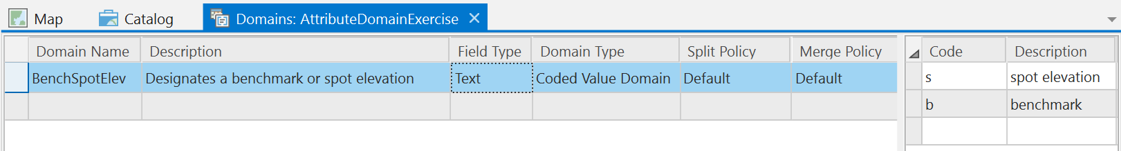 Figure 5.1: The Domains view, showing configuration of the BenchSpotElev coded value domain.
 - Do not close the Domains view. We still need to create our Range domain for elevation. In a new empty row, assign a Domain Name of ElevationRange and enter something appropriate for the Description.
- Change the Field Type to Long and set the Domain Type to Range. Do you know why we need to set the Domain type to Long?
- Now, in the panel to the right, you will see spaces in which to enter the Minimum value and the Maximum value that we wish to use to constrain the entries in the ELEVATION field in the attribute table of our Benchmarks feature class. For Minimum, enter 1000, and for Maximum enter 1900.
- Your range domain settings should look like the image below. Make sure they do, and hit the Save button.
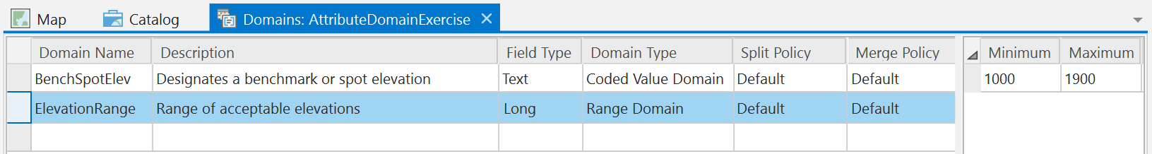 Figure 5.2: The Domains view showing configuration of the ElevationRange range domain.
 - Close the Domains view.
Now we need to apply the two new attribute domains to the BENCHSPOT and the ELEVATION fields. - Right-click on the Benchmarks feature class, and select Design > Fields.
- In the row for the ELEVATION field, access the dropdown list under the Domain heading and select the ElevationRange domain you just created.
 Figure 5.3: Assigning the ElevationRange domain to the ELEVATION field
 - Click the Save button. Do not close the Fields view.
- Now perform the same operation to assign the BenchSpotElev domain to the BENCHSPOT field.
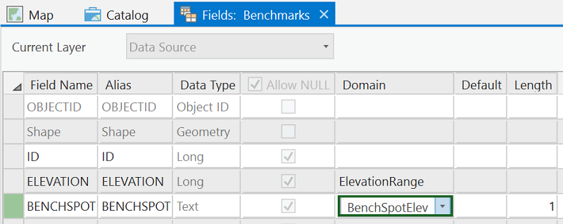 Figure 5.4: Assigning the BenchSpotElev domain to the BENCHSPOT field
 - Again, click the Save button.
And now you can close the Fields view.
Now, let's add the data to a map and see how the attribute domains help us control attribute data integrity. Before doing so, first a word about differences in attribute validation between ArcMap and ArcGIS Pro. In ArcMap, the default behavior is to allow values to be assigned to a field that are outside its domain. For example, you could enter an ELEVATION value greater than 1900, even after applying the ElevationRange domain. If that seems counter-intuitive to you, I would agree. However, ArcMap provides a Validate Features tool, which flags such invalid features so that you can correct them if you wish. And you also have the option of turning on automatic record validation, which will cause a warning to appear immediately if you attempt to enter a value outside a field's domain.
ArcGIS Pro, on the other hand, does not allow entries outside of a field's domain. I would say that's a sensible change. However, in a situation like this one, in which a domain has been applied after a feature class has already been populated with data, ArcMap's Validate Features tool provides a means to identify problematic values in the existing data, whereas ArcGIS Pro has no analogous tool.
- Add the Benchmarks feature class to the map and open its attribute table. You will probably notice immediately that the contents of the BENCHSPOT field appear different. While the code values that are a function of having assigned a coded value domain to a field are what are stored in the database, the description values are what display by default in the open attribute table. You can toggle this behavior off if you wish, clicking on the "hamburger" icon in the upper right of the table view and unchecking the Show domain and subtype descriptions option.
- Try changing one of the ELEVATION values to something greater than 1900 and note that it immediately reverts to the maximum allowed value (1900) per the domain we imposed.
- Click on a BENCHSPOT cell and note that you are limited to the two options defined in the BenchSpotElev domain (or Null).
- Next, click the Switch button to switch from no features selected to all features selected.
- Under the Edit tab, click the Attributes button. This will open a panel in which all of the benchmark features are listed by their ID value in the top of the panel and the full set of attributes for the currently highlighted feature is listed in the bottom of the panel.
- Click on ID 108 and note that its ELEVATION value is highlighted in red because that value is outside the field's domain. Click on ID 119 and note that both its ELEVATION and BENCHSPOT values are highlighted in red for the same reason.
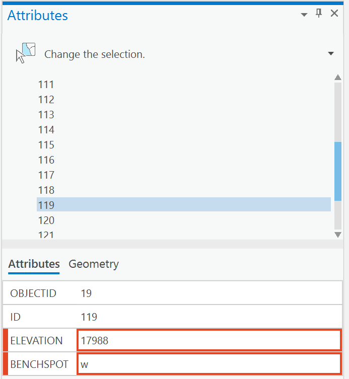 Figure 5.5: Attributes panel in ArcGIS Pro, showing attribute values violating attribute domain rules that are in place.
Clicking on features one at a time looking for attributes highlighted in red is not a particularly exciting prospect, especially if you're dealing with a lot more than the 25 features we have in this exercise. Better options would be to:
a. Use the Validate Features tool in ArcMap to isolate the problematic records, or
b. Use the Select By Attributes tool to find them (e.g., BENCHSPOT NOT IN ('b', 's') and ELEVATION < 1000 OR ELEVATION > 1900).
In any case, this problem of fixing invalid attribute values can be avoided if you apply domains when you first create the feature class!
B. Split and Merge Policies
Additional behaviors that can accompany attribute domains allow us to define what values get assigned to the field when a feature is split into two or when two features are merged into one. According to the Esri documentation, "...merge policies are not evaluated when merging features in the Editor. However, developers can take advantage of merge policies when writing their own merge implementations." The scope of this lesson does not include developer-level exercises, so we will visit only the use of split policies.
- In ArcGIS Pro's Catalog View, navigate to the AttributeDomainExercise.gdb file geodatabase and Preview the Roads feature class. We will be working with the SurfaceType field and the Length_Feet field.
Note that the Length_Feet field is a Float type field, and the SurfaceType field is a Text type field.
Let's create a coded value domain to use with the SurfaceType field and a range domain to use with Length_Feet field. - Right-click on the AttributeDomainExercise.gdb file geodatabase, and open its Domains view (Design > Domains).
- Click in the cell beneath your ElevationRange domain name, and name a new domain LengthFeet, and describe it as Length range in feet.
- Set the Field Type to Float (do you recall why?), and set the Domain Type to Range.
- Now, from the dropdown list under the Split policy heading, choose Geometry Ratio. This setting will make it so that the resulting values (in feet) in the Length_Feet field are in the same ratio as that of the lengths (the geometry) of the two new line features that resulted from the split operation.
Take note of the other two choices in the Split policy picklist. The Default Value is taken from the Default Value property that can be assigned to the field. We will see this below in the context of the coded value domain for the SurfaceType field. In this case, it would not make much sense to assign a default length to road segments, nor would it make sense to use the other choice, Duplicate, to assign the same length to each segment.
We will not interact with the Merge policy setting since we cannot take advantage of it, as mentioned above. But go ahead and look at the choices given if you are curious. - Let's define the Minimum value as 10 and the Maximum value as 264000. We are arbitrarily deciding that when we split a line feature representing a road that no road segment can be shorter than 10 feet or longer than 50 miles (264,000 feet).
- Check to be sure your settings are correct, and hit the Save button, but do not close the Domains view.
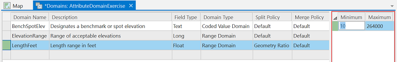 Figure 5.6: Defining a domain with a Split Policy setting.
 - Next, let's set up a domain for the road surface type values. Name it RoadSurface and describe it as Road surface material.
- Set the Field Type to Text. Note that this will force the Domain Type to be set to Coded Value Domain. But you knew that would be the case, right?
- Then set the Split policy to Default. As mentioned above, the default value is specified later in the properties of the SurfaceType field.
(The only Merge policy setting for a coded value domain is Default.) - Now, because this is a coded value domain, we need to enter the Code values and the corresponding Description values. Recall that we learned in the previous section that the codes are stored in the database (and the descriptions appear in the open table). As you noted when you previewed the data in the SurfaceType field of the Roads feature class, the existing data values are grass, gravel, asphalt, concrete and cobblestone. We will go ahead and retain those as the code values and set the description values to match. A "code" does not have to be a numeral or a single character (like the s and b used for the Benchmarks above). So go ahead and enter the five surface type category names in the right-hand panel as shown in the figure below. Take care to spell the code entries correctly. A misspelling would result in the existing values in the SurfaceType field not taking part in the domain.
- Hit the Save button when certain you have entered the correct settings -- the RoadSurface domain settings should look like this:
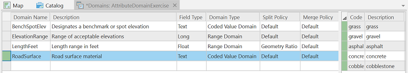 Figure 5.7: RoadSurface domain settings, with the Split Policy set to Default.
 - Close the Domains view.
Now, let's assign the two new domains to the respective fields in the Roads feature class attribute table. - Still in Catalog View, right-click on the Roads feature class and select Design > Fields to open the Fields view.
- You've done this before. Under the Domain heading, click on the Length_Feet cell and select LengthFeet from the dropdown list.
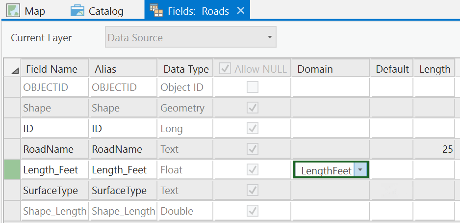 Figure 5.8: Assigning the LengthFeet domain to the Length_Feet field.
 - Hit Save.
- Next, assign the RoadSurface domain to the SurfaceType field. Note that the BenchSpotElev domain also appears in the picklist. Why, do you suppose?
- Also, under the Default heading, type asphalt. Recall that above we set the Split policy for the RoadSurface domain to Default Value. We are now specifying that default value; it needs to be one of the Code values that is part of the RoadSurface domain. Spell it correctly.
We can say that we know that most of the future work on the road system in this area will be done by the State, so the "asphalt" surface type is most apt to be involved; hence, we can set it as the default.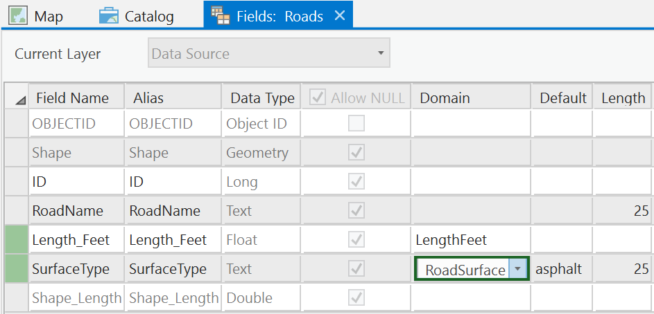 Figure 5.9: Assigning the RoadSurface domain to the SurfaceType field, and setting the Default value to 'asphalt', and the Length to 25.
 - Hit Save, then close the Fields view.
Now, let's see the behavior imposed on the data by two domains when we perform some edits. - Add the Roads feature class to the map.
- Open the Roads feature class attribute table.
- Select the U.S. Hwy 62 feature; you can click on it in the attribute table. Note the Length_Feet value (23128.34), and the SurfaceType value (concrete).
- Under the Edit tab, select the Split Tool and arbitrarily choose a point on the selected line feature and perform a split.
What happens? If you performed the split successfully, you should now see two separate U.S. Hwy 62 line features on the map and two U.S. Hwy 62 records in the attribute table.
What happened to the SurfaceType value for both of the features that are now the U.S. Hwy 62? Are they still "concrete"? Why not?
What are the Length_Feet values for the two features? Do they add up to 23128.34?
You can use the Undo tool in the upper right of the application window to revert to pre-split status if you want to compare the before and after. - Experiment with editing some of the other features if you wish.
- Save your project if you want, and quit ArcGIS Pro.
C. Project - Attribute Domains
For the homework deliverable for this part of the lesson, I am going to have you create two attribute domains to be assigned to existing fields in a feature class attribute table.
The data you will use is found in the AttributeDomainsProject.gdb file geodatabase. That geodatabase contains a single feature class named BuildingFootprints.
- Create an attribute domain and assign it to the Bldg_Type field (alias Building Type). The three allowed values for the field include C (commercial), R (residential), and P (public). NULL values are also allowed when the building category is not known.
- The Bldg_Story field (alias Building Stories) should contain values no larger than 7. Create and assign an attribute domain that will allow you to verify that values in that field do not violate that stipulation.
- Using either the Validate Features tool in ArcMap or your own queries in ArcGIS Pro, make and submit a screen capture showing features that have values outside the two domains. The image should show the selected offending records in the attribute table along with the query you used to select them.
- Submit your AttributeDomainsProject.gdb file geodatabase to the Lesson 5 drop box.
Following are some instructions on how to zip up both your image file and your AttributeDomainsProject.gdb file geodatabase.
In Lesson 5, we are dealing with File Geodatabases. Your AttributeDomainsProject.gdb geodatabase is a folder even though it has the .gdb extension on the name. To compress your file geodatabase along with your screen captured image in order to submit them, do the following:- In a Windows Explorer or a (My) Computer window, select both the geodatabase folder and your Word document file. The assumption is that the geodatabase and the image file are in the same folder making it possible to select them both.
- Then right-click on one of them and choose Send To | Compressed (zipped) Folder.
That will create a .zip file in the same folder. You need to turn in this .zip file. If, for some reason, you do not have the option to compress from within the Windows operating system, you can download a free application called 7-Zip [32]. It works well. - Name your .zip file appropriately, something like: <your name>_Lesson5Domains.zip.
D. Summary
Because attribute domains are stored in the geodatabase, they can be used by any dataset: feature class, table, subtype (covered in the next part of the lesson), within the geodatabase.
You can now move on to the Subtypes part of the lesson.
Subtypes
Subtypes
In a situation where we have a lot of similar features, roads for example, that we want to easily assign separate attribute values to and symbolize differently, etc., we can designate them as what Esri calls subtypes. The alternative for managing such data and information would be to create separate feature classes for, in this example, each type of road. This practice can affect the performance and ease of use of the database.
Subtypes can be created for spatial features in a feature class or for objects (records) in a nonspatial, stand alone table. Subtypes can be created based on an existing field or a new field is created to hold the subtype values.
A subtype is defined by a code and a description. The codes are stored in a field in the attribute table and must be either Short or Long Integer values. Each code value is equated to a descriptive category. Sounds a lot like a coded value domain but, as you will see, they are not the same.
In our exercise example, we will be creating road subtypes from integer values that represent six different road type categories.
Follow this link to download the data for this part of the lesson: Subtypes.zip [33]
The zip archive contains two Esri file geodatabases:
- SubtypesExercise.gdb
- SubtypesProject.gdb
A. Assigning features to subtypes
We are going to place roads in subtype categories according to the values in an existing field that contains integer values that represent six road type categories.
- Open ArcGIS Pro.
- Navigate to the SubtypesExercise.gdb geodatabase in the Catalog pane and take note of its two attribute domains: MaintPeriod and RoadSurface.
- Now look into the Roads feature class that resides in the SubtypesExercise.gdb geodatabase. Investigate the attribute data and the properties of the fields. The data in the RoadType field will be the basis for our subtypes, and we will see how attribute domains are involved, too.
As mentioned above, an existing field containing either Long or Short Integer values can be used as the basis for establishing subtypes. The integer values 1 - 6 in the RoadType field represent the following categories of road. Each will become a subtype within our Roads feature class.- 1 - Primary Hwy
- 2 - Secondary Hwy
- 3 - Light Duty
- 4 - Unimproved
- 5 - 4WD
- 6 - Trail
- Let's use those descriptions to establish our subtypes. Open the Subtypes View for the Roads feature class (right-click, select Design > Subtypes).
- Click the Create/Manage button on the ribbon to begin creating the subtype.
- In the Manage Subtypes dialog that appears, select RoadType as the Subtype Field.
- Skipping over the Default Subtype for now, let us proceed to enter the Code values and their corresponding Description values using the list of road types above.
- The Default Subtype should be automatically set to Primary Hwy, assuming it was the first subtype you entered. But let's assume that we know that a roads improvement project will be beginning that will result in new Light Duty type roads being created. So, let's change the Default Subtype to Light Duty.
Your Manage Subtypes dialog should look like this: Figure 5.10: Defining the Roads subtypes using the Manage Subtypes dialog.
 - Click OK to finishing creating the subtypes.
Upon clicking OK, you should see new headings appear in the Subtypes View, one for each of the subtypes. The Light Duty heading will be in bold, indicating that it's the default subtype. Beneath each heading, you should see two columns: Domain and Default Value. As you can probably guess, this enables you to configure each subtype to have its own domain and default value, if desired. - Notice that, by default, the first subtype listed has become the Default Subtype. Let's change that.
- Under the Primary Hwy heading, make the following settings:
- specify the Default Value for the Surface Type field by selecting concrete from the dropdown list
- assign the MaintPeriod range domain to the MaintPeriod field (yes, the domain and the field have the same name)
- specify a Default Value of 2 (months) for the MaintPeriod field
- For each subtype, proceed to set a default value for the Surface Type field, assign the MaintPeriod range domain to the MaintPeriod field, and set a default value for the MaintPeriod field. Do so according to the following list.
- Primary Hwy | SurfaceType = concrete | MaintPeriod = 2 (already taken care of above)
- Secondary Hwy | SurfaceType = concrete | MaintPeriod = 2
- Light Duty | SurfaceType = asphalt | MaintPeriod = 6
- Unimproved | SurfaceType = cobblestone | MaintPeriod = 8
- 4WD | SurfaceType = gravel | MaintPeriod = 12
- Trail | SurfaceType = grass | MaintPeriod = 12
- Your Subtypes View should look like the following. (The green bars indicate settings that haven't been saved.)
 Figure 5.11 The Subtypes View with domains and default values set for each subtype.
 - Be sure to click Save to apply your settings, then you may close the Subtypes View.
Now we will see what the implementation of the subtypes has put at our disposal. - If you haven't already, add the Roads feature class to the map.
One thing that is an implication of having subtypes assigned will be readily apparent. In the Contents pane, you will see that each subtype is listed along with a distinct symbolization. Go ahead and alter the symbol for each road type if you wish.
 Figure 5.12: The Contents pane in ArcGIS Pro, showing the subtypes of the Roads feature class.
 - Now, click the Edit tab, followed by the Create button. In the Create Features pane that opens, notice that each subtype has its own editing template. This serves to reinforce that each subtype is a category unto itself.
 Figure 5.13: The Create Features pane, showing that each subtype of the Roads feature class has an editing template.
 - Go ahead and choose one of the Roads subtype editing templates, then sketch a new line feature. It doesn't need to be a real road, you're simply testing out the subtype behavior. When you complete the sketch of the new line feature, a new record appears in the attribute table, complete with the default values pertinent to whatever subtype category you chose.
- Experiment further if you wish. Save your edits if you wish.
- Close ArcGIS Pro, saving your project if you desire.
So instead of creating separate feature classes for the different road types, we put the road line features into subtypes which gave us the ability to specify unique default values for each new feature of a different road type category, and to assign, or not, certain attribute domains to each category.
B. Project - Subtype Creation
As was mentioned above, subtypes can be created for objects (records) in a nonspatial table. In this homework project, that is what you will do.
Investigate the field structure and attribute data in the Encounters table residing in the SubtypesProject.gdb geodatabase. In addition to the OBJECTID field that is automatically created by the GIS, you will find the following five fields: ID, Encounter, Category, EducationLevel, and BloodAlcohol.
The values of 1 and 2 in the Encounter field represent Distant Encounters and Close Encounters respectively.
The descriptions of the values in the Category field are as follows:
- DE-1 - Nocturnal Light
- DE-2 - Daylight Disc
- DE-3 - Radar-visual
- CE-1 - Light/object in Proximity
- CE-2 - Physical Trace
- CE-3 - Occupant
The encounter data descriptions are based on information I took from the UFO Casebook site [34]: http://www.ufocasebook.com/Hynek.html
The values in the EducationLevel field are the number of years of school attended.
The values in the BloodAlcohol field are blood alcohol content measures. (Wikipedia Blood Alcohol Content Page [35]/ http://en.wikipedia.org/wiki/Blood_alcohol_content)
Here is what I want you to do for this project:
- Create an attribute domain for the three Distant Encounter categories (the DE values)
- Create an attribute domain for the three Close Encounter categories (the CE values)
- Create an attribute domain for the education level data
- Create an attribute domain for the blood alcohol content data
- Create subtypes based on the values in the Encounter field and associate the appropriate attribute domains with each
- Based on the data choose a default subtype (in spite of the small sample size)
- Based on the data specify default values for the two encounter subtypes (again, in spite of the small sample size)
When finished, zip your SubtypesProject.gdb geodatabase and submit it to the Project 5 Drop Box.
It can be problematic if the result of zipping your file geodatabase results in an archive name like Sloan_SubtypesProject.gdb.zip -- the embedded .gdb needs to be avoided.
Geodatabase Topology
Geodatabase Topology
A geodatabase topology is another construct that is stored within a geodatabase and gives us added control over assessing and maintaining the integrity of our spatial data.
Follow this link to download the data for this part of the lesson: Topology.zip [36]
The zip archive contains the following:
An Esri File Geodatabase: geodatabasetopol.gdb
A zip archive: TopologyProject.zip
Controlling spatial data integrity by imposing rules - Geodatabase Topology
A geodatabase topology provides a robust way of defining topological relationships among spatial features. It does so by analyzing coordinate locations of feature vertices both among features within a feature class and between features in multiple feature classes taking part in the topology. Therefore, it is not only important that all of the feature classes participating in a geodatabase topology be in the same coordinate system, but also that the measurement precision defined for each feature class be the same. To assure that this is the case, all feature classes that take part in a geodatabase topology must reside within what is known as a Feature Dataset. When a feature dataset is created, the coordinate system and precision are defined, and any subsequent feature class that is added to the feature dataset inherits that coordinate system and precision. In the exercise that follows, you will see that the precision is controlled by the Tolerance and Resolution settings. I encourage you to read more about these topics in the Topology in ArcGIS [37] entry in the ArcGIS Pro documentation.
A geodatabase topology is governed by topology "rules" that the user specifies, and those rules are based on knowledge of the relationships between and among the features that will be taking part in the topology. So, the onus is on the user to understand the data being created/edited in order that appropriate rules are specified.
The manifestation of a geodatabase topology is as a layer in the feature dataset. As such, the topology errors that it contains are symbolized just as are the features in any other map layer in ArcGIS. In the documentation, the Validate and fix geodatabase topology [38] topic provides an overview of the error fixing process along with links to the rules available for points, polylines, and polygons. If you are inclined to adorn your walls with GIS help guides, you may want to print the topology rules poster [39]. Whether you print it out or not. it offers a bit more in the way of graphic description and examples of the rules.
Once topology rules have been imposed on the data in a feature dataset. errors are discovered by "validating" the topology. Validation can be done on the entire visible extent of the data or on a smaller specified area. The latter technique allows you to just check an area that you have been editing, rather than the entire dataset. This can save time when the entire dataset is large.
As is mentioned above, one needs to be aware of how the features involved in a geodatabase topology relate to each other in order to be able to define appropriate topology rules to govern the creation of spatial data and aid in discovering errors in existing data. In the following exercise, we will be working with the data depicted in the image below, and I will be the arbitrary source of what is known about the relationships among the features in the four feature classes involved. We will be basing our choices of rules on the following:
- the polygons in the FDpolygon_1 feature class must have a single point feature within them
- all of the polygons in the FDpolygon_1 feature class must be within the polygons (there is only one) in the FDpolygon_2 feature class
- the polygons in the FDpolygon_1 feature class must have no gaps between them
- the polygons in the FDpolygon_1 feature class must not overlap
- all of the lines in the FDline feature class must be within the FDpolygon_2 polygons
- all of the lines in the FDline feature class cannot be joined to only one other line feature in the feature class (In topology parlance, the point where only two line segments meet is called a pseudo-node, or -vertex.)
- where lines in the FDline feature class meet, they must be snapped together (The end of a line feature that is not connected to another line feature is said to dangle.)

A. Create and interact with a Geodatabase Topology
- Open ArcGIS Pro.
- In the Catalog pane, navigate to your geodatabasetopol.gdb geodatabase.
- Within the geodatabasetopol.gdb geodatabase is a feature dataset named TopolExFeatureDataset. Verify that it contains four feature classes. You might also check the XY Coordinate System and the Tolerance and the Resolution of some of the feature classes to see that those settings are indeed the same for each feature class.
- Right-click on the TopolExFeatureDataset and select New > Topology. This will start the Create Topology Wizard.
- Accept the defaults for the name and for the cluster tolerance.
- Click the Select All button to include all of the feature classes in the feature dataset to the topology that we are creating.
We'll now assign a rank value to each feature class. The lower the number, the higher the rank. A high rank value indicates that positions of the features in that feature class are known more accurately, or that we do not want them to move relative to feature classes of lower rank during an editing operation. - Assign a value of 4 to the Number of XY Ranks property.
- Let's arbitrarily assign the following ranks (though nothing we do in the steps that follow will illustrate the effect of the rankings):
- 1 - FDpolygon_1
- 2 - FDpolygon_2
- 3 - FDline
- 4 - FDpoint
- Click Next. We're presented with an empty table of topology rules. Now, based on our knowledge and understanding of how the spatial data in the feature classes are topologically related, we can specify the rules that help us to ensure that those spatial relationships are maintained. Click in the empty row at the bottom of the table to add a new rule. Add each of the rules listed below, in all cases setting Feature Class 1 and a Rule, and sometimes setting Feature Class 2. Subtypes do not apply in this scenario.
- FDpoint | Must Be Properly Inside | FDpolygon_1
- FDpolygon_1 | Must Be Covered By Feature Class Of | FDpolygon_2
- FDpolygon_1 | Must Not Have Gaps
- FDpolygon_1 | Must Not Overlap
- FDline | Must Be Inside | FDpolygon_2
- FDline | Must Not Have Pseudo Nodes
- FDline | Must Not Have Dangles
- Click Next. You can review the choices just made.
Click Finish.
After processing for a few moments, you should have a new geodatabase topology layer named TopolExFeatureDataset_Topology in your TopolExFeatureDataset feature dataset. - In the Catalog pane, right-click on the topology layer and select Add to Current Map. This will add the topology layer and the four feature classes participating in the topology. (Yes, the data oddly cover much of the western hemisphere. I haven't the slightest idea where these shapes came from, please just go with it.)
The topology layer should display at the top of the Table of Contents list. This is important in order to be able to view the topology errors when they are symbolized. See Figure 5.16, below. - Alter the symbology and rearrange the order of the 4 feature class layers in order to clearly see the features they contain.
Do not label the features yet. - Under the Edit tab, in the Manage Edits group, you should see your geodatabase topology selected in the dropdown list. If not, go ahead and select it. Note that while we're experimenting with a geodatabase topology here, it is also possible to instead store topology rules as part of a map within a Pro project.
- Click on the Error Inspector
 button. The Error Inspector will display beneath the map by default.
 Figure 5.15: The Error Inspector pane.
 - We're now going to validate the topological relationships according to the rules we defined. First, be certain you can view all of the features in the map display area. The validation will be carried out only for the features visible in the current map extent by default. Click the Validate button (part of the Error Inspector GUI).
Several features in the colors indicated in the Table of Contents pane for the topology layer should be visible. We will spend the next several steps investigating what they tell us.
(The image below also shows the results of the feature labeling we will do in the next step.)
 Figure 5.16: The map, showing the TopolExFeatureDataset_Topology geodatabase topology, along with the layers that take part in the geodatabase topology. The image also shows the labeling of the features.
 - Before we proceed, let's label the features in the data frame with the values in the OBJECTID field of each feature class. For each layer, right-click, select Labeling Properties, set the Expression to $feature.OBJECTID, then right-click on the layer again and select Label.
- Keep in mind what you read above, at the beginning of this section, in regard to what are the desired spatial relationships of the features in the dataset we are working with.
The Error Inspector shows errors associated with all rules by default, but we can limit that to just a particular rule. Next to the Filter heading, click the Rules button, and select FDline - Must Not Have Pseudo Nodes.
The full list of 19 errors will be reduced to 2. - Click on the row in the Error Inspector that holds the error entry where Feature 1 is 10 and Feature 2 is 16. The Feature # is the value of the OBJECTID field. This is why I had you label the features with the values in the OBJECTID field.
This type of error is represented by a Point Error symbol, the pink square. When you click the row in the Error Inspector, the pink square that separates line features 10 and 16 will turn yellow, thus indicating the location of the instance that violates this particular topological rule, that each line feature in the FDline feature class should share an end point with at least two other lines. The highlighted error indicates a situation where only two line features are sharing an endpoint. Note that you are also shown a zoomed-in look at the error in the right-hand pane of the Error Inspector. - If you right-click on the line entry in the Error Inspector, it will bring up a list (see Figure 5.17 below) from which you can choose to, among several things, Merge or Merge To Largest. These are two choices in the context of this particular type of error for fixing the problem. The Merge choice gives you an option to choose one of the two line features. The implication is that the attributes associated with the chosen line will be those retained for the new single line feature that results from the Merge.
Go ahead and experiment with the choices in the list. You can always Undo any change you make. (Ctrl-Z, or use the Undo button in the upper left of the application window)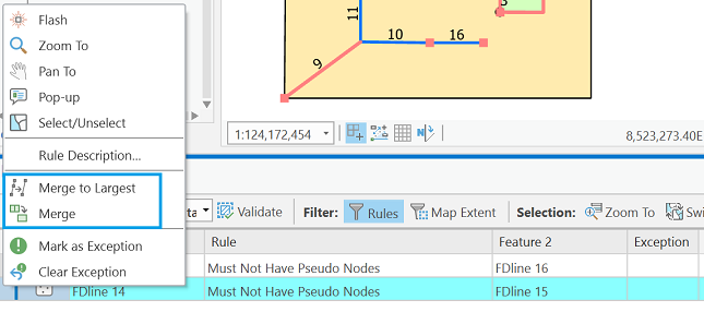 Figure 5.17: The menu that comes up when you right-click on an entry of the Error Inspector pane.
 - There is a second violation of the Must Not Have Pseudo Nodes error. Highlight it via the Error Inspector. You'll see that it is where line features 8, 14, and 15 are supposed to meet. If you zoom in far enough on that intersection, you will see that line 8 is not snapped at the intersection of lines 14 and 15.
- It turns out that one of our other rules would have also highlighted an error in that same area. Do you know which one? Click the Rules button again and select FDline - Must Not Have Dangles.
- In the list of errors, click the row where Feature 1 is equal to 8. That should also highlight a vertex in the vicinity of where line feature 8 is supposed to be snapped at the intersection of lines 14 and 15. Which vertex is highlighted? It is the end vertex of line feature 8.
The list of Must Not Have Dangles errors contains 10 entries. It is important to realize that not all dangling line feature endpoints are actually errors. It is acceptable to have dead end streets, for example. - It is also important to realize that the Must Not Have Dangles rule only pertains to features in a single layer. If you click through the list of dangle errors, you will see that three of the entries on the list are where line features 7, 8, and 9 meet the corners of polygon 11 (the FDpolygon_2 feature). If you do some investigating, you will find that the end of line 7 is indeed snapped to the corner vertex of polygon 11. Even so, the geodatabase topology still flags it as a possible error.
- Now, let's look at the FDpolygon_1 - Must Not Have Gaps error results.
Select it from the Rules picklist in the Error Inspector. You should see two results listed in the Error Inspector represented by the Line Error symbol. - One of the Error Inspector entries, when chosen from the list, will show the result depicted in the image below (Figure 5.18).
Click on the entries until you find it.
Part of the description of this topology rule includes the following: "An error will always exist on the perimeter of the surface. You can either ignore this error or mark it as an exception." Figure 5.18: The view of the FDpolygon_1 data after you choose the desired Must Not Have Gaps entry in the Error Inspector.
 - Let's mark this as an exception.
Right-click on the error entry in the Error Inspector table and choose Mark As Exception. An exclamation point icon will appear in the Exception column and if you select a different error, you'll see that what had been a pink outline, indicating an error, has changed to a green outline, indicating that it's been marked as an exception. - Select the error that highlights the boundary between polygons 2 and 5, then click the Error Inspector's Zoom To button. Toggle the topology layer's visibility off for the moment so that you're able to see the polygon boundaries. When you zoom in far enough, you should discover a gap between FDpolygon_1 polygons 2 and 5. Someone did not do a good job of making sure the FDpolygon_1 features shared boundaries.
Let's stick with the FDpolygon_1 polygon layer and perform an edit. While we are at it, we will learn how to highlight areas in our data that have been modified/edited. These "dirty areas," as they are referred to, let us know that we should validate the topology again. - Zoom back out to Full Extent.
In the Error Inspector, select the FDpolygon_1 - Must Not Overlap rule. There should be two errors. We are going to focus on the one involving polygons 2 and 3. - Again making sure the topology layer is turned off, zoom in on the location of the overlap error between polygons 2 and 3 until you have a good view of the overlap. You could elect to change the display of the layer to "Hollow" in order to see the overlap more definitely.
- Let's rectify the overlap using the canned error correction choice provided by the Error Inspector. Right-click on the error in the Error Inspector and select Merge from the menu.
- In the Merge window that opens, click on each of the two entries. Doing so will cause the polygon that the overlap area will be merged with to be flicker-highlighted.
- Choose the first of the two -- for polygon feature 2, and then click the Merge button.
- If you still have the display of the TopolExFeatureDataset_Topology layer un-checked, check the box now. Also turn on the display of the Dirty Areas Polygon 3 should be highlighted in the hatch pattern, indicating that it is a dirty area -- that a change has been made since the topology rules were last validated.
- Click the Validate button again. The hatched area should disappear, indicating that the error has been correctly dealt with as far as our topology rules are concerned. Also note that there should be only one overlap error left.
- You should save your edits now (Edit > Save).
- Deliverable- I want to see that you were able to perform the correction we just went though, so zip up your geodatabasetopol.gdb geodatabase and upload it to the Project 5 Drop Box.
You should be getting a feel for how to interact with the Error Inspector.
Go ahead and spend some time investigating the other rules infractions to see if you can determine the reasons for the other error symbols that you see on the map.
- Why is there a Point Error at the bottom-left corner of the FDpolygon_1 polygon 5 feature (point 3)?
- Why is line 9 highlighted?
- etc.
If you want, attempt to correct some of the other errors. Not all of them (like the gap we found between the two polygons) have canned fixes via the Error Inspector. So if you are pining away for a chance to do some editing, be my guest.
I leave it up to you to choose whether or not to save the project, and any edits you make.
B. Using topology editing tools with shared polygon boundaries
With a geodatabase topology in place, there are certain tools at your disposal that enable you to maintain topological relationships when you make edits to spatial data. Here, we contrast editing a shared polygon boundary with and without having a geodatabase topology set up. It is important to realize that the "shared" boundary between two polygons actually is a duplicate set of line segments, each polygon boundary exists as complete and independent from the adjacent polygon. So, when a shared boundary needs to be edited, one must actually edit the boundaries of two polygons.
- First, we will look at the case where we have no topology imposed on the data, and we attempt to edit a shared polygon boundary with the Vertices tool
 . The images below illustrate what happens. Because the edit is conducted with No Topology, only one of the polygon's vertices can be moved at a time. The images depict a simple case, but think of a situation where three or four polygons share a common corner vertex.
 Figure 5.19: Two polygon features in a geodatabase feature class that share a boundary.
 Figure 5.20: The result of editing/moving one vertex when conducted with No Topology.
 - With a topology in place, the capabilities of the Vertices tool are extended a bit. In the Modify Features pane to the right of the map, an Edges tab appears in addition to the Features tab. By clicking the Edges tab, you can then select a shared edge that you'd like to modify. In the first of the two figures below, the shared edge is shown selected after having clicked the Edges tab. In the second figure, you can see that the same vertex moved in Figure 5.20 has been moved again. This time, both polygon boundaries are edited at the same time.
 Figure 5.21: With a geodatabase topology in place, and the shared boundary selected prior to moving the vertex.
 Figure 5.22: The result of editing/moving two shared vertices when a geodatabase topology is in place.
C. Project - Given a single feature class in a geodatabase, set up a geodatabase topology and deal with a single class of error
Because this is not a course in inputting and editing spatial and attribute data, we are choosing to focus on what needs to be done to prepare to implement a geodatabase topology. There will be some errors in spatial data to repair, but it involves going over ground already covered in section A of the lesson.
Unzip the TopologyProject.zip archive. The archive contains a folder named TopologyProject. Within that folder is a geodatabase (TopologyProject.gdb) and a georeferenced image of a map (with ancillary files).
The BuildingFootprints feature class contains some instances of polygon overlap that need to be repaired.
In order for you to accomplish finding and repairing the errors in the BuildingFootprints feature class, you are going to have to create and employ a geodatabase topology. You know from section A how to create a geodatabase topology, and you know that in order to do so, the data in question has to reside within a feature dataset. What we did not explicitly go over in the lesson was how to (1) create a feature dataset, and (2) how to get existing data, in this case the feature class contained in the TopologyProject.gdb, into a feature dataset that we create. But that's what I want you to do. Given that Geography 484 or comparable experience was the prerequisite for taking this course, you should be able to do it.
Once you have accomplished that, proceed to find and correct the overlapping building footprint polygons. All of the offending features will be in the area covered by the included georeferenced map image. You can use it as reference to make sure you are performing the corrections to the polygons correctly.
When you finish, zip up your version of the TopologyProject.gdb and upload it to the Lesson 5 Drop Box.
Attribute Domains (for ArcMap)
Attribute Domains
In Geography 484: GIS Database Development, you were introduced to attribute domains; however, it is possible to go through that course without having actually implemented them. So we will go over Coded Value Domains and Range Domains in the following section. Some of the material will be review for some of you, but even if you did work with attribute domains in Geography 484, you are apt to be exposed to functionality associated with them that was not covered in that course.
Follow this link to download the data for this part of the lesson: AttributeDomains.zip [29]
The zip archive contains two Esri File Geodatabases:
- AttributeDomainExercise.gdb
- AttributeDomainProject.gdb
A. Coded Value and Range Domains
A coded value domain allows you to choose from a list of values that are allowed in a field. A range domain allows you to specify a valid range for values in a numeric field. Both types of attribute domain thus provide means of enforcing data integrity.
- Open ArcCatalog (the standalone application, not the Catalog window in ArcMap), and look at the Properties of the Benchmarks feature class found in the AttributeDomainExercise.gdb file geodatabase. Right-click and choose Properties. Click the Fields tab and take note of the Data Type of the ELEVATION field and of the BENCHSPOT field. Close the Feature Class Properties window.
Also Preview the feature class, use the picklist at the bottom of the Preview pane to view the contents of the attribute Table.
The point features in the feature class represent locations of elevation benchmarks and spot elevations. The BENCHSPOT field is meant to hold an s for a spot elevation or a b for a benchmark location. A quick perusal of the values in that field shows that there are some errors. In addition, the elevation in this region ranges from about 1000 feet to about 1900 feet above sea level. We can see that there are some values in the ELEVATION field that violate that range. Our summer intern was not very meticulous.
Let's create and impose a coded value domain that will limit the possible entries in the BENCHSPOT field to s and b. And let's create and impose a range domain on the ELEVATION field that will allow us to verify that the values in that field are within the correct elevation range.
First, we will create a coded value domain named BenchSpotElev. - Right-click on the name of the AttributeDomainExercise.gdb file geodatabase and select Properties. This will open the Database Properties window.
Select the Domains tab. - In the first open slot under Domain Name, type BenchSpotElev. Then in the corresponding Description slot, enter a brief description of your choice.
- Look at the entries in the Domain Properties area. The cell next to Domain Type will let you select either Coded Values or Range. We are creating a coded value domain, so make sure it is set to the Coded Values choice.
- We know that the values in the existing BENCHSPOT field are Text type; so now in the Domain Properties area, click in the cell to the right of Field Type, and from the picklist choose Text. While we are here, note that based on the choices in the picklist, you can create a coded value domain that can be used with six different field data types.
After setting the Field Type to Text, the Domain Type will no longer present the Range choice; a Range domain can only be a numeric type. - Now in the Coded Values area, we must enter both Code values and corresponding Description values. The values s and b will be our code values, and the respective descriptions will be spot elevation and benchmark.
Your Database Properties window should look like the image below. Your domain Description may be different, and hopefully without the typo that mine has. - If all is as it should be, hit the Apply button; this is important to do before we move on.
Note: If you have a set of codes and associated descriptions in tabular form already, you can avoid the trouble of re-entering that information as outlined above by using the Table to Domain tool [30]. And if you are looking to automate the domain pieces of a workflow through either Model Builder or Python scripting, you may want to check out the other tools in the Domains toolset [31].
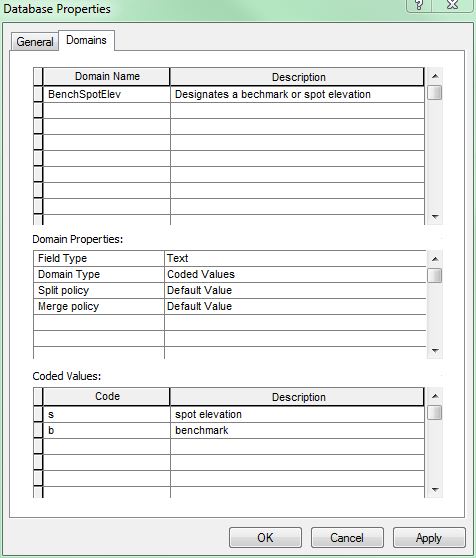 Figure 5.1: The Database Properties dialog > Domains tab configuration for the BenchSpotElev coded value domain.
 - Do not close the Database Properties window. We still need to create our Range domain for elevation. Go back to the Domain Name column and add an entry named ElevationRange and enter something appropriate for the Description.
- Change the Field Type to Long Integer and set the Domain Type to Range. Do you know why we need to set the Domain type to Long Integer?
- Now you will see spaces in which to enter the Minimum value and the Maximum value that we wish to use to constrain the entries in the ELEVATION field in the attribute table of our Benchmarks feature class. For Minimum value, enter 1000, and for Maximum value enter 1900.
- Your range domain setting should look like those below. Make sure they do, and hit the Apply button.
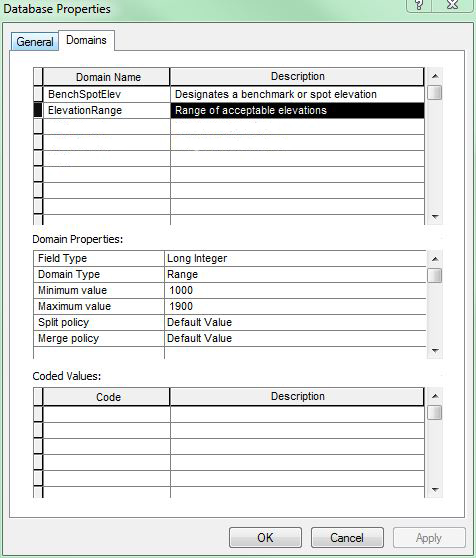 Figure 5.2: The Database Properties dialog > Domains tab configuration for the ElevationRange range domain.
 - Hit the OK button to close the Database Properties window.
Now we need to apply the two new attribute domains to the BENCHSPOT and the ELEVATION fields. - Right-click on the Benchmarks feature class, and select Properties.
Select the Fields tab if necessary. - Click on the ELEVATION field name. In the Field Properties area, there should be a Domain property.
Click in the cell next to it, and select the ElevationRange domain.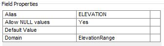 Figure 5.3: Assigning the ElevationRange domain to the ELEVATION field.
 - Click the Apply button. Do not close the Feature Class Properties window.
- Now, click on the name of the BENCHSPOT field.
In the cell next to the Domain property, choose the BenchSpotElev domain.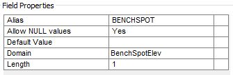 Figure 5.4: Assigning the BenchSpotElev domain to the BENCHSPOT field, and setting the Length property to 1.
 - Again, click the Apply button.
And you can click the OK button to dismiss the window.
Now, let's go into ArcMap and see how the attribute domains help us control attribute data integrity. In an editing session, with the desired features selected, we can find out if there are any attribute entries that violate the specifications of the attribute domains we established. - Open ArcMap.
- Add the Benchmarks feature class to the data frame and open its attribute table. You will probably notice immediately that the contents of the BENCHSPOT field appear different. While the code values that are a function of having assigned a coded value domain to a field are what are stored in the database, the description values are what display by default in the open attribute table. You can control the display by going into the Table Properties menu (the icon in the upper left), selecting Appearance and checking or un-checking the box for Display coded value domains and subtype descriptions.
- Start an editing session. Add the Editor toolbar if necessary.
- From the Table Options list in the open attribute table, choose Select All.
- Now, from the Editor drop down list on the Editor toolbar, select Validate Features. Two things will happen. You will see a popup that lets you know that there are five features with attribute values in violation of the attribute domain rules, and the selected set of features will be reduced to those five offending features.
At this point, you could go ahead and deal with the errors by editing the values in the attribute table.
 Figure 5.5: Popup showing how many attribute values violate attribute domain rules that are in place.
 - When it comes to adding additional features and corresponding attributes with the coded value domain in place for the BENCHSPOT field, a drop-down list from which either valid value can be chosen will appear when that cell in the attribute table is edited. When it comes to the ELEVATION field, you can either periodically perform the Validate Features step as we did above, or you can go into the Table Options menu > choose Appearance | and check the box for Automatically validate records. With that set, a warning will appear any time you enter an elevation value that is not within the specified range.
Take some time and experiment. - Close ArcMap. You can save your map document if you wish. You may want to return to it.
B. Split and Merge Policies
Additional behaviors that can accompany attribute domains allow us to define what values get assigned to the field when a feature is split into two or when two features are merged into one. According to the Esri documentation, "...merge policies are not evaluated when merging features in the Editor. However, developers can take advantage of merge policies when writing their own merge implementations." The scope of this lesson does not include developer-level exercises, so we will visit only the use of split policies.
- In ArcCatalog, navigate to the AttributeDomainExercise.gdb file geodatabase and Preview the Roads feature class. We will be working with the SurfaceType field and the Length_Feet field.
View the Feature Class Properties of the Roads feature class, and see that the Length_Feet field is a Float type field, and the SurfaceType field is a Text type field.
Let's create a coded value domain to use with the SurfaceType field and a range domain to use with Length_Feet field. - Right-click on the AttributeDomainExercise.gdb file geodatabase, and go to Properties.
Select the Domains tab. - Click in the cell beneath your ElevationRange domain name, and name a new domain LengthFeet, and describe it as Length range in feet.
- In the Domain Properties area, set the Field Type to Float (do you recall why?), and set the Domain Type to Range.
- Let's define the Minimum value as 10 and the Maximum value as 264000. We are arbitrarily deciding that when we split a line feature representing a road that no road segment can be shorter than 10 feet or longer than 50 miles (264,000 feet).
- Now, from the picklist in the cell next to Split policy, choose Geometry Ratio. This setting will make it so that the resulting values (in feet) in the Length_Feet field are in the same ratio as that of the lengths (the geometry) of the two new line features that resulted from the split operation.
Take note of the other two choices in the Split policy picklist. The Default Value is taken from the Default Value property that can be assigned to the field. We will see this below in the context of the coded value domain for the SurfaceType field. In this case, it would not make much sense to assign a default length to road segments, nor would it make sense to use the other choice, Duplicate, to assign the same length to each segment.
We will not interact with the Merge policy setting since we cannot take advantage of it, as mentioned above. But go ahead and look at the choices given if you are curious. - Check to be sure your settings are correct, and hit the Apply button, but do not close the Database Properties window.
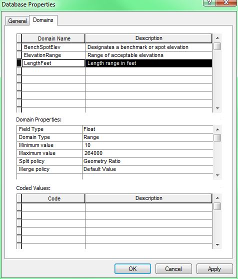 Figure 5.6: Domain Properties > Domains tab showing settings to create LengthFeet range domain, with the Split policy property set to Geometry Ratio.
 - Next, let's set up a domain for the road surface type values. Name it RoadSurface and describe it as Road surface material.
- Set the Field Type to Text. Note that this will force the Domain Type to be set to Coded Values. But you knew that would be the case, right?
- Then set the Split policy to Default Value. As mentioned above, the default value is specified later in the properties of the SurfaceType field.
(The only Merge policy setting for a coded value domain is Default value.) - Now, because this is a coded value domain, we need to enter the Code values and the corresponding Description values. Recall that we learned in the previous section that the codes are stored in the database (and the descriptions appear in the open table). As you noted when you previewed the data in the SurfaceType field of the Roads feature class the existing data values are grass, gravel, asphalt, concrete and cobblestone. We will go ahead and retain those as the code values and set the description values to match. A "code" does not have to be a numeral or a single character (like the s and b used for the Benchmarks above). So go ahead and enter the five surface type category names in both the Code list and the Description list of the Coded Values area. Take care to spell the code entries correctly. A misspelling would result in the existing values in the SurfaceType field not taking part in the domain.
- Hit the Apply button when certain you have entered the correct settings -- the RoadSurface domain settings should look like this:
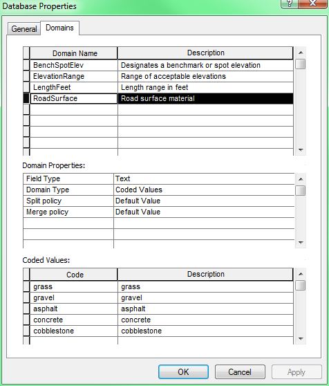 Figure 5.7: Domain Properties > Domains tab showing settings to create RoadSurface coded value domain, with the Split policy set to Default Value.
 - Hit the OK button to dismiss the Database Properties window.
Now, let's assign the two new domains to the respective fields in the Roads feature class attribute table. - Still in ArcCatalog, right-click on the Roads feature class and select Properties to open the Feature Class Properties window.
- You've done this before, In the Field Name list, click on the Length_Feet field, then in the Field Properties area assign the LengthFeet domain to the Domain property of the field.
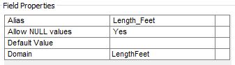 Figure 5.8: Assigning the LengthFeet domain to the Length_Feet field.
 - Hit Apply.
- Next, click the SurfaceType field, and assign the RoadSurface domain to it. Note that the BenchSpotElev domain also appears in the picklist. Why, do you suppose?
- Also, in the cell next to Default Value in the Field Properties area, type asphalt. Recall that above we set the Split policy for the RoadSurface domain to Default Value. We are now specifying that default value; it needs to be one of the Code values that is part of the RoadSurface domain. Spell it correctly.
We can say that we know that most of the future work on the road system in this area will be done by the State, so the "asphalt" surface type is most apt to be involved; hence, we can set it as the default.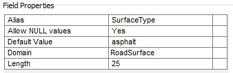 Figure 5.9: Assigning the RoadSurface domain to the SurfaceType field, and setting the Default Value to 'asphalt', and the Length property to 25.
 - Hit Apply, then hit OK.
Now, in ArcMap, let's see the behavior imposed on the data by two domains when we perform some edits. - Open ArcMap, and add the Roads feature class to the data frame.
- Open the Roads feature class attribute table.
- Start an editing session.
- Select the U.S. Hwy 62 feature; you can click on it in the attribute table. Note the Length_Feet value (23128.34), and the SurfaceType value (concrete).
- Select the Split Tool from the Editor toolbar, and arbitrarily choose a point on the selected line feature and perform a split. You might want to invoke the Edge Snapping to aid you.
What happens? If you go to select the U.S. Hwy 62 line feature, it should be in two parts, and there should also be a new record in the attribute table at the bottom.
What happened to the SurfaceType value for both of the features that are now the U.S. Hwy 62? Are they still "concrete"? Why not?
What are the Length_Feet values for the two features? Do they add up to 23128.34?
You can use the Undo tool on the standard toolbar to revert to pre-split status if you want to compare the before and after. - Experiment with editing some of the other features if you wish.
- Save your map document if you want, and quit ArcMap.
C. Project - Attribute Domains
For the homework deliverable for this part of the lesson, I am going to have you create two attribute domains to be assigned to existing fields in a feature class attribute table.
You will use the behavior functionality that the domains give you to find several attribute errors that reside in the dataset.
The data you will use is found in the AttributeDomainsProject.gdb file geodatabase. That geodatabase contains a single feature class named BuildingFootprints.
- Create an attribute domain for the Bldg_Type field (alias Building Type). The three allowed values for the field include C (commercial), R (residential), and P (public). NULL values are also allowed when the building category is not known.
- The Bldg_Story field (alias Building Stories) should contain values no larger than 7. Create an attribute domain that will allow you to verify that values in that field do not violate that stipulation.
- Make and submit a screen capture showing the results of discovering the errors that exist in the two fields in question. The image should show (1) the selected offending records in the attribute table, and (2) the popup showing the number of offending records.
- Submit your AttributeDomainsProject.gdb file geodatabase to the Lesson 5 drop box.
Following are some instructions on how to zip up both your image file and your AttributeDomainsProject.gdb file geodatabase.
In Lesson 5, we are dealing with File Geodatabases. Your AttributeDomainsProject.gdb geodatabase is a folder even though it has the .gdb extension on the name. To compress your file geodatabase along with your screen captured image in order to submit them, do the following:- In a Windows Explorer or a (My) Computer window, select both the geodatabase folder and your Word document file. The assumption is that the geodatabase and the image file are in the same folder, making it possible to select them both.
- Then right-click on one of them and choose Send To | Compressed (zipped) Folder.
That will create a .zip file in the same folder. You need to turn in this .zip file. If, for some reason, you do not have the option to compress from within the Windows operating system, you can download a free application called 7-Zip [32]. It works well. - Name your .zip file appropriately, something like: <your name>_Lesson5Domains.zip.
D. Summary
Because attribute domains are stored in the geodatabase, they can be used by any dataset: feature class, table, subtype (covered in the next part of the lesson), within the geodatabase.
You can now move on to the Subtypes part of the lesson.
Subtypes (for ArcMap)
Subtypes
In a situation where we have a lot of similar features, roads for example, that we want to easily assign separate attribute values to and symbolize differently, etc., we can designate them as what are called Subtypes. The alternative for managing such data and information would be to create separate feature classes for, in this example, each type of road. This practice can affect the performance and ease of use of the database.
Subtypes can be created for spatial features in a feature class or for objects (records) in a nonspatial, standalone table. Subtypes can be created based on an existing field, or a new field is created to hold the subtype values.
A subtype is defined by a code and a description. The codes are stored in a field in the attribute table and must be either Short or Long Integer values. Each code value is equated to a descriptive category. Sounds a lot like a coded value domain but, as you will see, they are not the same.
In our exercise example, we will be creating road subtypes from integer values that represent six different road type categories.
Follow this link to download the data for this part of the lesson: Subtypes.zip [33]
The zip archive contains two Esri File Geodatabases:
- SubtypesExercise.gdb
- SubtypesProject.gdb
A. Assigning features to subtypes
We are going to place roads in subtype categories according to the values in an existing field that contains integer values that represent six road type categories.
- Open ArcCatalog.
- Navigate to the SubtypesExercise.gdb geodatabase and take note of the two attribute domains: MaintPeriod and RoadSurface.
- Now look into the Roads feature class that resides in the SubtypesExercise.gdb geodatabase. Investigate the attribute data and the properties of the fields. The data in the RoadType field will be the basis for our subtypes, and we will see how attribute domains are involved, too.
As mentioned above, an existing field containing either Long or Short Integer values can be used as the basis for establishing subtypes. The integer values 1 - 6 in the RoadType field represent the following categories of road. Each will become a subtype within our Roads feature class.- 1 - Primary Hwy
- 2 - Secondary Hwy
- 3 - Light Duty
- 4 - Unimproved
- 5 - 4WD
- 6 - Trail
- Let's use those descriptions to establish our subtypes. Open the Feature Class Properties dialog window for the Roads feature class.
- Select the Subtypes tab. Take a look at the aspects involved in defining subtypes. Note the area of the dialog that allows us to set default values for fields and to specify attribute domains. Such settings will be imposed on our existing features and upon new features that we create, providing a measure of automated data integrity control. There are also a Domains button that allows us to review the attribute domains that exist in our geodatabase. This can come in handy when we want to set default values.
- In the Subtype Field dropdown list, select the RoadType field. Recall that it contains the integer values that will become the codes for our subtypes. Also note that the names of the fields in the feature class and any assigned domains are now visible.
- Let us now proceed to provide the Code values and the corresponding Description values for the subtypes. First, replace the 0 in the Code column with a 1, and then change New Subtype to Primary Hwy. Then, using the list of road types above, continue to supply code and description values in the Subtypes area. You can hit the Apply button at any time along the way to preserve your progress of establishing the settings.
- Notice that, by default, the first subtype listed has become the Default Subtype. Let's change that. Assume that we know that a roads improvement project will be beginning that will result in new Light Duty type roads being created. So, let's change the Default Subtype to Light Duty.
- Now, let's spend some time specifying the behavior of each subtype by modifying the settings for each via the Default Values and Domains area. One at a time, we will select each subtype in the Subtypes list and then specify settings for it in the Default Values and Domains area. In order to highlight one of the subtypes in the list, click on the small gray box at the left end of the row. Clicking anywhere in the row of one of the subtypes will select it but won't highlight it and so makes it harder to remember which one we are interacting with.
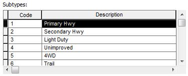 Figure 5.10: The Primary Hwy domain highlighted, by clicking on the small box on the left end of the row..
 - Select the Primary Hwy subtype, then, in the Default Values and Domains area, do three things:
- specify the Default Value for the Surface Type field by typing in concrete
- the MaintPeriod range domain was not assigned to the MaintPeriod field (yes, the domain and the field have the same name), so we can do that now -- click in the Domain cell in the MaintPeriod field row, and choose the MaintPeriod domain
- specify a Default Value of 2 (months) for the MaintPeriod field
- For each subtype, proceed to set a default value for the Surface Type field, assign the MaintPeriod range domain to the MaintPeriod field, and set a default value for the MaintPeriod field. Do so according to the following list. Don't forget that you can hit the Apply button at any time during the process to save your progress.
- Primary Hwy | SurfaceType = concrete | MaintPeriod = 2 (already taken care of above)
- Secondary Hwy | SurfaceType = concrete | MaintPeriod = 2
- Light Duty | SurfaceType = asphalt | MaintPeriod = 6
- Unimproved | SurfaceType = cobblestone | MaintPeriod = 8
- 4WD | SurfaceType = gravel | MaintPeriod = 12
- Trail | SurfaceType = grass | MaintPeriod = 12
The image below shows the dialog window with the Trail subtype chosen.
 Figure 5.11: The Subtypes dialog with the Trail subtype chosen. Then the Default Value and Domain are selected for the Surface Type and MaintPeriod fields.
- When you are finished, hit the OK button to dismiss the dialog window.
Now, we will go into ArcMap and see what the implementation of the subtypes has put at our disposal. - Open ArcMap and add the Roads feature class to the data frame.
One thing that is an implication of having subtypes assigned will be readily apparent. In the table of contents window, you will see that each subtype is listed along with a distinct symbolization. Go ahead and alter the symbol for each road type if you wish.
 Figure 5.12: The Table of Contents pane in ArcMap, showing the subtypes of the Roads feature class.
 - Now, initiate an edit session. In the Create Features window that opens, notice that each subtype has its own editing template. This serves to reinforce that each subtype is a category unto itself.
 Figure 5.13: The Create Features pane, showing that each subtype of the Roads feature class has an editing template.
 - Let's do something we've done before.
Still in an editing session, open the Roads feature class attribute table.
From the Table Options menu, Select All features. - Now, go to the Editor pull down list on the Editor toolbar and Validate Features.
You should discover that there are 4 violations. What are these based on? In each case, the MaintPeriod value is outside the range specified in the range domain assigned to that field. If you do not get a report of four errors, you may have neglected to assign the MaintPeriod domain to the field of the same name up above.
This reporting of attribute value violations can point to potential problems in the existing data, ones that are less apt to occur in the future now that we have exerted some control over the integrity of data that will be newly created in the context of our subtype settings. - While you are still in the editing session with the attribute table still open, create a new road feature:
- Click on one of the Roads subtypes templates in the Create Features window. Doing so will turn your mouse cursor into the Line construction tool, see beneath the Create Features window.
- Digitize a line feature
- Experiment further if you wish. Save your edits if you wish.
- Close ArcMap, saving your map document if you desire.
So instead of creating separate feature classes for the different road types, we put the road line features into subtypes which gave us the ability to specify unique default values for each new feature of a different road type category, and to assign, or not, certain attribute domains to each category.
B. Project - Subtype Creation
As was mentioned above, subtypes can be created for objects (records) in a nonspatial table. In this homework project, that is what you will do.
Investigate the field structure and attribute data in the Encounters table residing in the SubtypesProject.gdb geodatabase. In addition to the OBJECTID field that is automatically created by the GIS, you will find the following five fields: ID, Encounter, Category, EducationLevel, and BloodAlcohol.
The values of 1 and 2 in the Encounter field represent Distant Encounters and Close Encounters respectively.
The descriptions of the values in the Category field are as follows:
- DE-1 - Nocturnal Light
- DE-2 - Daylight Disc
- DE-3 - Radar-visual
- CE-1 - Light/object in Proximity
- CE-2 - Physical Trace
- CE-3 - Occupant
The encounter data descriptions are based on information I took from the UFO Casebook site [34]: http://www.ufocasebook.com/Hynek.html
The values in the EducationLevel field are the number of years of school attended.
The values in the BloodAlcohol field are blood alcohol content measures. (Wikipedia Blood Alcohol Content Page [35]/ http://en.wikipedia.org/wiki/Blood_alcohol_content)
Here is what I want you to do for this project:
- Create an attribute domain for the three Distant Encounter categories (the DE values)
- Create an attribute domain for the three Close Encounter categories (the CE values)
- Create an attribute domain for the education level data
- Create an attribute domain for the blood alcohol content data
- Create subtypes based on the values in the Encounter field and associate the appropriate attribute domains with each
- Based on the data, choose a default subtype (in spite of the small sample size)
- Based on the data, specify default values for the two encounter subtypes (again, in spite of the small sample size)
When finished, zip your SubtypesProject.gdb geodatabase and submit it to the Project 5 Drop Box.
It can be problematic if the result of zipping your file geodatabase results in an archive name like Sloan_SubtypesProject.gdb.zip -- the embedded .gdb needs to be avoided.
Geodatabase Topology (for ArcMap)
Geodatabase Topology
A geodatabase topology is another construct that is stored within a geodatabase and gives us added control over assessing and maintaining the integrity of our spatial data.
Follow this link to download the data for this part of the lesson: Topology_ArcMap.zip [40]
The zip archive contains the following:
An Esri Personal Geodatabase: geodatabasetopol.mdb
A zip archive: TopologyProject.zip
Controlling spatial data integrity by imposing rules - Geodatabase Topology
A geodatabase topology provides a robust way of defining topological relationships among spatial features. It does so by analyzing coordinate locations of feature vertices, both among features within a feature class and between features in multiple feature classes taking part in the topology. Therefore, it is not only important that all of the feature classes participating in a geodatabase topology be in the same coordinate system, but also that the measurement precision defined for each feature class be the same. To assure that this is the case, all feature classes that take part in a geodatabase topology must reside within what is known as a Feature Dataset. When a feature dataset is created, the coordinate system and precision are defined, and any subsequent feature class that is added to the feature dataset inherits that coordinate system and precision. In the exercise that follows, you will see that the precision is controlled by the Tolerance and Resolution settings. I encourage you to read more about these topics in the Desktop Help when you have time. Search on "topology rules", and then select the "Topology in ArcGIS" topic entry.
A geodatabase topology is governed by topology "rules" that the user specifies, and those rules are based on knowledge of the relationships between and among the features that will be taking part in the topology. So, the onus is on the user to understand the data being created/edited in order that appropriate rules are specified. Rules can be added to and taken away from a topology as long as the data is not part of an active ArcMap editing session.
The manifestation of a geodatabase topology is as a layer in the feature dataset. As such, the topology errors that it contains are symbolized just as are the features in any other map layer in ArcMap. In the Desktop Help, search on "topology rules", and then select the "Geodatabase topology rules and topology error fixes" topic entry. This will take you to a compilation of the types of rules that can be defined along with suggestions for ways to fix violations of each rule and a description of how the errors are symbolized in the map data frame, as Points, Lines, and Areas. If you are inclined to adorn your walls with GIS help guides, you will find a link to a topology rules poster in the opening passage to the Help page I just referred you to. Whether you print it out or not. it offers a bit more in the way of graphic description and examples of the rules.
Once topology rules have been imposed on the data in a feature dataset. errors are discovered by "validating" the topology. Validation can be done on the entire visible extent of the data or on a smaller specified area. The latter technique allows you to just check an area that you have been editing, rather than the entire dataset. This can save time when the entire dataset is large.
As is mentioned above, one needs to be aware of how the features involved in a geodatabase topology relate to each other in order to be able to define appropriate topology rules to govern the creation of spatial data and aid in discovering errors in existing data. In the following exercise, we will be working with the data depicted in the image below, and I will be the arbitrary source of what is known about the relationships among the features in the four feature classes involved. We will be basing our choices of rules on the following:
- the polygons in the FDpolygon_1 feature class must have a single point feature within them
- all of the polygons in the FDpolygon_1 feature class must be within the polygons (there is only one) in the FDpolygon_2 feature class
- the polygons in the FDpolygon_1 feature class must have no gaps between them
- the polygons in the FDpolygon_1 feature class must not overlap
- all of the lines in the FDline feature class must be within the FDpolygon_2 polygons
- all of the lines in the FDline feature class cannot be joined to only one other line feature in the feature class (In topology parlance, the point where only two line segments meet is called a pseudo-node, or -vertex.)
- where lines in the FDline feature class meet, they must be snapped together (The end of a line feature that is not connected to another line feature is said to dangle.)

A. Create and interact with a Geodatabase Topology
- Open ArcCatalog.
- Navigate to your geodatabasetopol.mdb geodatabase.
- Within the geodatabasetopol.mdb geodatabase is a feature dataset named TopolExFeatureDataset, and within it are four feature classes. Verify this, and Preview the data in the feature classes if you wish. You might also check the XY Coordinate System and the Tolerance and the Resolution of the some of the feature classes to see that those settings are indeed the same for each feature class.
- Right-click on the TopolExFeatureDataset name | expand New| select Topology. This will start the New Topology wizard.
Click Next. - Accept the defaults for the name and for the cluster tolerance. Click Next.
- In the next window, click the Select All button to include all of the feature class layers in the geodatabase topology that we are creating.
- Click Next. We now have the option to assign a rank value to each feature class. The lower the number, the higher the rank. A high rank value indicates that positions of the features in that feature class are known more accurately, or that we do not want them to move relative to layers of lower rank during an editing operation. Let's arbitrarily assign the following ranks (though nothing we do in the steps that follow will illustrate the effect of the rankings):
- 1 - FDpolygon_1
- 2 - FDpolygon_2
- 3 - FDline
- 4 - FDpoint
- Click Next. Now based on our knowledge and understanding of how the spatial data in the feature classes are topologically related, we need to specify the rules that help us to ensure that those spatial relationships are maintained. To comply with the relationships among the features that we outlined above, use the Add Rule... button to choose the following rules:
- FDpoint | Must Be Properly Inside | FDpolygon_1
- FDpolygon_1 | Must Be Covered By Feature Class Of | FDpolygon_2
- FDpolygon_1 | Must Not Have Gaps
- FDpolygon_1 | Must Not Overlap
- FDline | Must Be Inside | FDpolygon_2
- FDline | Must Not Have Pseudo Nodes
- FDline | Must Not Have Dangles
- Click Next. You can review the choices just made.
Click Finish.
It will process for a moment and then ask if you would "...like to validate it now?" - Click No. We will validate the topological relationships later in ArcMap.
Now within your TopolExFeatureDataset feature dataset, there will be a geodatabase topology "layer" named TopolExFeatureDataset_Topology. - Open ArcMap, and initiate a new map document.
- You will need the Topology toolbar and the Editor toolbar, so add them to the display if they are not already there.
- Expand the Catalog pane. (If you do not see the tab on the upper-right side, go to the Windows menu and select Catalog.)
Navigate into the TopolExFeatureDataset. - Drag-and-drop the TopolExFeatureDataset_Topology into your data frame.
Click Yes when it asks if you want to add the feature classes that participate in the topology.
The topology layer should display at the top of the Table of Contents list. This is important in order to be able to view the topology errors when they are symbolized. See Figure 5.16, below. - Alter the symbology and rearrange the order of the 4 feature class layers in order to clearly see the features they contain.
Do not label the features yet. - Start an editing session. This will awaken the Topology toolbar.
You can hide the Create Features pane (click the push pin icon). - Take note of the components on the Topology toolbar.
- The icon on the far-right end of the Topology toolbar invokes the Error Inspector. Click it.
The Error Inspector will display beneath the data frame by default. Resize your ArcMap window as needed in order to see it.
 Figure 5.15: The Error Inspector pane.
 - Recall that when we created the geodatabase topology in ArcCatalog, we chose not to validate the topological relationships at that time. Let's do that now. First, be certain you can view all of the features in the map display area. You literally need to be able to see the features -- it isn't enough that they are in the data frame, if they are in the data frame but covered by the Error Inspector pane for example, they will not be validated.
The Validate Topology in Current Extent tool is the third icon from the right end of the Topology toolbar.
Click it.
Several features in the colors indicated in the Table of Contents pane for the topology layer should be visible. We will spend the next several steps investigating what they tell us.
(The image below also shows the results of the feature labeling we will do in the next step.)
 Figure 5.16: The map document, showing the TopolExFeatureDataset_Topology geodatabase topology added to the data frame, along with the layers that take part in the geodatabase topology. The image also shows the labeling of the features.
 - Before we proceed, let's label the features in the data frame with the values in the OBJECTID field of each feature class. For each layer, bring up the Layer Properties window | select the Labels tab | change the Label Field to OBJECTID | click OK. Then right-click on the layer name in the table of contents and select Label Features.
- Keep in mind what you read above, at the beginning of this section, in regard to what are the desired spatial relationships of the features in the dataset we are working with.
Expand the Show: picklist in the Error Inspector, and choose FDline - Must Not Have Pseudo Nodes, and then click the Search Now button. NOTE: It is still important that all of the features still be visible in the data frame.
Two entries will appear in the Error Inspector table. - Click on the row in the Error Inspector that holds the first error entry, where Feature 1 is 10 and Feature 2 is 16. The Feature # is the value of the OBJECTID field. This is why I had you label the features with the values in the OBJECTID field.
This type of error is represented by a Point Error symbol, the pink square. When you click the row in the Error Inspector, the pink square that separates line features 10 and 16 will turn black, thus indicating the location of the instance that violates this particular topological rule, each line feature in the FDline feature class should share an end point with at least two other lines. The highlighted Point Error indicates a situation where only two line features are sharing an endpoint. - If you right-click on the line entry in the Error Inspector, it will bring up a list (see Figure 5.17 below) from which you can choose to, among several things, Merge or Merge To Largest. These are two choices in the context of this particular type of error for fixing the problem. The Merge choice gives you an option to choose one of the two line features. The implication is that the attributes associated with the chosen line will be those retained for the new single line feature that is a result of the Merge.
Go ahead and experiment with the choices in the list. You can always Undo any change you make. (Ctrl-Z, or Edit menu | Undo... or use the Undo... tool icon.)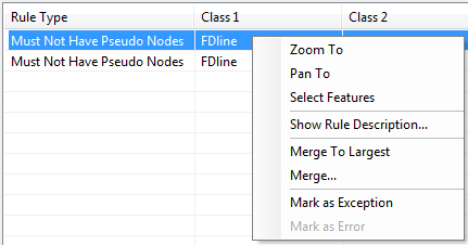 Figure 5.17: The menu that comes up when you right-click on an entry of the Error Inspector pane.
 - There is a second violation of the Must Not Have Pseudo Nodes error. Highlight it via the Error Inspector. You'll see that it is where line features 8, 14, and 15 are supposed to meet. If you zoom in far enough on that intersection, you will see that line 8 is not snapped at the intersection of lines 14 and 15.
- It turns out that one of our other rules would have also highlighted an error in that same area. Do you know which one? Expand the Show: picklist in the Error Inspector, and choose FDline - Must Not Have Dangles, and then click the Search Now button.
- In the list of errors, click the first row where Feature 1 is equal to 8 (it ought to be third from the bottom). That should also highlight a vertex in the vicinity of where line feature 8 is supposed to be snapped at the intersection of lines 14 and 15. Which vertex is highlighted? It is the end vertex of the 8 line feature.
The list of Must Not Have Dangles errors contains 10 entries. It is important to realize that not all dangling line feature endpoints are actually errors. It is acceptable to have dead end streets for example. - It is also important to realize that the Must Not Have Dangles rule only pertains to features in a single layer. If you click through the list of ten dangle errors, you will see that three of the entries on the list are where line features 7, 8, and 9 meet the corners of polygon 11 (the FDpolygon_2 feature). If you do some investigating, you will find that the end of line 7 is indeed snapped to the corner vertex of polygon 11. Even so, the geodatabase topology still flags it as a possible error. To prove to yourself that line 7 is snapped to the polygon boundary, you may need to invoke a Map Topology. Do you recall how from having taken Geography 484?
- Now, let's look at the FDpolygon_1 - Must Not Have Gaps error results.
Select it from the Show: picklist in the Error Inspector.
Then hit the Search Now button. You should see two results listed in the Error Inspector represented by the Line Error symbol. - One of the Error Inspecctor entries, when chosen from the list, will show the result depicted in the image below (Figure 5.18).
Click on the two entries until you find it.
Part of the description of this topology rule includes the following: "An error will always exist on the perimeter of the surface. You can either ignore this error or mark it as an exception."
 Figure 5.18: The view of the FDpolygon_1 data after you chose the desired Must Not Have Gaps entry in the Error Inspector.
 - Let's mark this as an exception.
Right-click on the error entry in the Error Inspector table and choose Mark As Exception. The pink lines marking the perimeter of each of the polygons will disappear and the error will disappear from the Errors list.
Note the Exceptions check box. You can search for things that you have marked as such if need be. - Highlight the remaining error on the list, take note of where it is (between polygons 2 and 5), and in the table of contents window, un-check the box controlling the display of the topology layer. This will prevent the topology features from hiding what we are looking for. When you zoom in far enough, you should discover a gap between FDpolygon_1 polygons 2 and 5. Someone did not do a good job of making sure the FDpolygon_1 features shared boundaries.
Let's stick with the FDpolygon_1 polygon layer and perform an edit. While we are at it, we will learn how to highlight areas in our data that have been modified/edited. These "dirty areas," as they are referred to, let us know that we should validate the topology again. - Zoom back out to Full Extent.
In the Error Inspector, show the FDpolygon_1 - Must Not Overlap error, and hit the Search Now button. There should be two errors. We are going to focus on the error involving polygons 2 and 3. - Turn off the display of the topology layer and zoom in on the location of the overlap error between polygons 2 and 3 until you have a good view of the overlap. You could elect to change the display of the layer to "Hollow" in order to see the overlap more definitely.
- Now, before we attempt to correct the error, go to the Layer Properties of the TopolExFeatureDataset_Topology layer | select the Symbology tab | check the box for Dirty Areas | click OK. A new "Dirty Areas" hatch symbol will appear in the table of contents under the topology layer.
- Let's rectify the overlap using the canned error correction choice provided by the Error Inspector. Right-click on the error in the Error Inspector and select Merge from the menu.
- In the Merge window that opens, click on each of the two entries. Doing so will cause the polygon that the overlap area will be merged with to be flicker-highlighted.
- Choose the first of the two -- the PLY12(FDpolygon_1) entry, and then click the OK button.
- If you still have the display of the TopolExFeatureDataset_Topology layer un-checked, check the box now. Polygon 3 should be highlighted in the hatch pattern, indicating that it is a dirty area -- that a change has been made since the topology rules were last validated.
- Zoom to full extent. We are going to use the Validate Topology In Specified Area tool
 (fourth from the end on the Topology toolbar) to see if the correction we made to the overlap is no longer considered an error. Select that tool and click-drag a rectangle that will encompass the hatched area. When you let off the mouse button, the hatched area should disappear, indicating that the error has been correctly dealt with as far as our topology rules are concerned.
To prove this to yourself, you can hit the Search Now button and see how many overlap errors are found. There should be only one left. - You should save your edits now.
- Deliverable- I want to see that you were able to perform the correction we just went though, so zip up your geodatabasetopol.mdb geodatabase and upload it to the Project 5 Drop Box.
You should be getting a feel for how to interact with the Error Inspector.
Go ahead and spend some time investigating the other rules infractions to see if you can determine the reasons for the other error symbols that you see on the map.
- Why is there a Point Error at the bottom-left corner of the FDpolygon_1 polygon 5 feature (point 3)?
- Why is line 9 highlighted?
- etc.
If you want, attempt to correct some of the other errors. Not all of them (like the gap we found between the two polygons) have canned fixes via the Error Inspector. So if you are pining away for a chance to do some editing, be my guest.
I leave it up to you to choose whether or not to save the map document, and any edits you make.
B. Using topology editing tools with shared polygon boundaries
With a geodatabase topology in place, there are certain tools at your disposal that enable you to maintain topological relationships when you make edits to spatial data. Here, we contrast editing a shared polygon boundary with and without having a geodatabase topology set up. It is important to realize that the "shared" boundary between two polygons actually is a duplicate set of line segments, each polygon boundary exists as complete and independent from the adjacent polygon. So when a shared boundary needs to be edited, one must actually edit the boundaries of two polygons.
- First we will look at the case where we have no topology imposed on the data, and we attempt to edit a shared polygon boundary with the Edit Vertices tool . The images below illustrate what happens. Because only one feature can be selected when editing with the Edit Vertices tool, only one instance of the extent of the shared boundary can be edited at a time. The images depict a simple case, but think of a situation where three or four polygons share a common corner vertex.
 Figure 5.19: Two polygon features in a geodatabase feature class that share a boundary.
 Figure 5.20: The result of editing/moving one vertex when no geodatabase topology is in place.
 - With a geodatabase topology in place, one can first use the Topology Edit Tool
 to select the length of the shared boundary. Then, using the Modify Edge tool
  (which when invoked causes the vertices to display), a shared vertex can be selected and moved, editing both polygon boundaries at the same time. Holding down the Shift key when selecting vertices allows you to select more than one.
 Figure 5.21: With a geodatabase topology in place, and the shared boundary selected using the Topology Edit Tool.
 Figure 5.22: The result of editing/moving two shared vertices when a geodatabase topology is in place.
C. Project - Given a single feature class in a geodatabase, set up a geodatabase topology and deal with a single class of error
Because this is not a course in inputting and editing spatial and attribute data, we are choosing to focus on what needs to be done to prepare to implement a geodatabase topology. There will be some errors in spatial data to repair, but it involves going over ground already covered in section A of the lesson.
Unzip the TopologyProject.zip archive. The archive contains a folder named TopologyProject. Within that folder is a map document (TopologyProject.mxd file), a geodatabase (TopologyProject.gdb) and a georeferenced image of a map (with ancillary files). When you unzip the archive, keep the folder and its contents intact. The map document is set to maintain relative paths to the data that it points to, so after you have extracted the folder and you navigate into it and double-click on the TopologyProject.mxd, the map image and the single feature class contained in the geodatabase should be present in the resulting ArcMap session.
The BuildingFootprints feature class contains some instances of polygon overlap that need to be repaired.
In order for you to accomplish finding and repairing the errors in the BuildingFootprints feature class, you are going to have to create and employ a geodatabase topology. You know from section A how to create a geodatabase topology, and you know that in order to do so, the data in question has to reside within a feature dataset. What we did not explicitly go over in the lesson was how to (1) create a feature dataset, and (2) how to get existing data, in this case the feature class contained in the TopologyProject.gdb, into a feature dataset that we create. But that's what I want you to do. Given that Geography 484 or comparable experience was the prerequisite for taking this course, you should be able to do it.
Once you have accomplished that, proceed to find and correct the overlapping building footprint polygons. All of the offending features will be in the area covered by the included georeferenced map image. You can use it as a reference to make sure you are performing the corrections to the polygons correctly.
When you finish, zip up your version of the TopologyProject.gdb and upload it to the Lesson 5 Drop Box.
Project 5: Esri Geodatabase Behaviors
Project 5: Esri Geodatabase Behaviors
A. Deliverables
This project is one week in length. Please refer to the Canvas Calendar for the due date.
The various Project deliverables were described along the way throughout the lesson. Below is a list summarizing what you need to submit.
- Attribute Domains - Upload your version of the AttributeDomainsProject.gdb geodatabase, and the screen capture showing the results of discovering the errors, both zipped into your last name_Lesson5_Domains.zip
- Subtypes - Upload your SubtypesProject.gdb geodatabase, zipped and named appropriately.
- Geodatabase Topology - (1) Upload your version of the geodatabasetopol.gdb geodatabase, and (2) your version of the TopologyProject.gdb, zipped and named appropriately. (I do not need your map document or any of the image files.)
- Complete the Lesson 5 quiz.
Lesson 6: Introduction to the Enterprise Geodatabase
Overview
Overview
Teaching enterprise geodatabase concepts online has historically been a challenge because it's been difficult to provide students with a "playground" to get hands-on experience. Fortunately, today it is much easier to give students hands-on experience with enterprise geodatabases through virtual machines hosted by Amazon. Over the next three weeks, you will use this Amazon cloud-based solution to set up and experiment with your own remote enterprise geodatabase server.
Objectives
At the successful completion of this lesson, students should be able to:
- set up a cloud-based enterprise geodatabase through Amazon's EC2 service;
- explain the concept of an Amazon Machine Image (AMI);
- stop and start their geodatabase instance;
- enable the transfer of files from their local machine to their geodatabase instance;
- describe the role of ArcSDE in allowing ArcGIS products to work with data in an RDBMS;
- list advantages of a multiuser (ArcSDE) geodatabase;
- connect to a SQL Server-based geodatabase through ArcGIS Desktop;
- create database login roles and assign data access privileges to those roles.
Questions?
If you have any questions now or at any point during this week, please feel free to post them to the Lesson 6 Discussion Forum.
Checklist
Checklist
Lesson 6 is one week in length. See the Canvas Calendar for specific due dates. To finish this lesson, you must complete the activities listed below. You may find it useful to print this page out first so that you can follow along with the directions.
- Work through Lesson 6.
- Complete the write-up of your organization's data users described on the last page of the lesson.
- Take Quiz 6.
Create a Cloud-Based Enterprise Geodatabase
Create a Cloud-Based Enterprise Geodatabase
Using the Amazon service mentioned above, Esri makes it possible to set up cloud-based installations of ArcGIS Enterprise, software required for implementing an enterprise geodatabase. Because our Cloud and Server GIS course also guides students through putting together an instance of ArcGIS Enterprise, the instructions below are borrowed from that course. While our focus in this course will be on the enterprise geodatabase that we'll implement on the instance with ArcGIS Enterprise, a side benefit is that you'll also be able to experiment with ArcGIS Enterprise functionality if you like.
A. Prepare to work in the Amazon cloud environment
Go to Amazon Web Services [41] and click on "Create an AWS Account."
If prompted to create a Business or Personal account, choose Personal. Please make careful note of the password you select when setting up your account, you will be needing it. It is characteristic of Amazon Web Services that things work the way they are supposed to, but you don't get a lot of hand-holding. So, if you lose your password, I'm not sure it would be easy to recover it, and you will need to fill out a form with personal information.
Second, you will need to provide payment information, including a credit card number. If you are careful and follow the course instructions about explicitly stopping your instance (virtual machine) when you are not using it, you should be able to complete the coursework while incurring charges of $20-$40. The current step of signing up is free, but you should be aware that you will start being charged immediately upon starting to use AWS services. As part of this step, you'll be asked to select a support plan. The Basic (Free) support is all you need for this class.
Third, there is an identity confirmation step during which you will receive a phone call and enter a code. This ensures you are a human. Amazon does not use the phone number provided here for other purposes.
You can monitor your billing status by clicking your user name at the top-right of the AWS screen and choosing "My Billing Dashboard." On the right side of the billing dashboard, you should see a "Month-to-Date Spend by Service" section, from which you can view details about what you're being charged for in the current month or any other month.
If any of these directions are confusing or inaccurate, please post a question or comment to the Lesson 6 discussion forum.
B. Create a VPC and key pair
In a few moments, we'll see that two of the settings involved in launching a new instance in EC2 are the VPC and key pair. A VPC (Virtual Private Cloud) is sort of your own special space carved out of Amazon's cloud. Instances in a VPC can see each other and your own network fairly easily, but they're not immediately accessible from elsewhere without some extra work on your part. That's a good thing for security.
A key pair is another security measure that will come into play when you log in to your instance for the first time. You will be logging in to your instance as a user named Administrator. The password for the Administrator user will be encrypted by AWS. The procedure for getting that password so that you can log in to your instance involves 1) creating a key pair (one key held by Amazon and another key given to you) in the AWS Management Console, 2) providing the name of that key pair when launching the instance, and 3) using the key pair after the instance has been created to decrypt the password.
Note: If you've taken our Cloud and Server GIS course (GEOG 865), you will have already created a VPC and key pair. You may skip over the steps in this section (or do them again if you like) and pick up with section C below.
- Go to the AWS Management Console [42] and click on VPC (under the Services > Networking & Content Delivery heading).
Creating a VPC is potentially a very technical and complex activity, but it's something most people have to do at first. For that reason, Amazon has made a wizard for setting up a real basic VPC. This will suffice for our purposes.
- Click Create VPC.
- Select the VPC and more option, then under the Name tag auto-generation heading confirm that the Auto-generate box is checked and enter a name tag of geog868. These two settings will automatically name some of the AWS resources that are about to be created.
- Set the Number of Availability Zones to 1. In a real-world implementation, you'd probably want at least two, but one should be fine for our classwork.
- Set the Number of public subnets to 1 and Number of private subnets to 0.
- Leave the other settings at their defaults and click Create VPC.
- After a few moments, AWS should be done doing its thing, and you can click the View VPC button.
When we launch our instance in a few moments, we want it to be assigned a public IP address so that we can connect to it using Windows Remote Desktop. Whether the instance is assigned a public IP address or not depends on whether the subnet we just created allows for that. The default setting is for it to not assign one, but that's something we can change. - Under the Virtual Private Cloud heading in the left-hand pane of the console, click on the Subnets link. You'll see just one subnet listed, unless you've created a VPC/subnet before.
- In any case, you want to right-click on the named subnet and choose Edit subnet settings.
- Check the Enable auto-assign public IPv4 address box and click Save.
With a VPC and subnet created and configured, let's turn our attention to the key pair.
- Go to the EC2 Management Console [43] (click the link to the left or select Services > Compute > EC2) and under the Network & Security heading click on the Key Pairs link in the navigation pane on the left side of the page.
- Click Create Key Pair.
- Give it a Name (e.g., geog868_keypair) and change the file format to .pem. Then click Create.
- Save the .pem file produced by AWS to a folder on your machine where you'll be able to find it later. (It will likely be automatically saved to your Downloads folder. You may want to move it to a location where you're less likely to delete it mistakenly.)
C. Create your own cloud-based instance of ArcGIS Enterprise
Esri provides two ways to deploy ArcGIS in AWS: using Amazon's CloudFormation service and Amazon's AWS Management Console. For our purposes, the AWS Management Console is the best option, so we will lead you through the launching of an instance via that route. However, if you decide to deploy ArcGIS in the cloud as part of your job, you may want to explore the CloudFormation option as well. Instructions for both can be found in Esri's documentation [44] [http://server.arcgis.com/en/server/latest/cloud/amazon/use-aws-management-console-with-arcgis-server.htm]. Note that this link opens the Management Console instructions; instructions for the CloudFormation method can be found through the navigation headings on the left side of the page.
The basic idea behind what we're about to do is that Amazon has made it possible for vendors like Esri to create machine images (configurations of operating system, software, data, etc.) that can serve as blueprints for the making of child instances. Esri has created several of these AMIs (Amazon Machine Images): one that runs ArcGIS Enterprise on the Linux OS Ubuntu with Postgres, one that runs ArcGIS Enterprise on Windows with SQL Server, etc. Third parties (like us) can discover and "subscribe" to these AMIs through the AWS Marketplace.
- Browse to the AWS Marketplace description of the ArcGIS Enterprise 10.9.1 AMI [45] [https://aws.amazon.com/marketplace/pp/prodview-rh32a6tw3ju4a?sr=0-3&ref_=beagle&applicationId=AWSMPContessa].
- In the upper right, click the Continue to Subscribe button. You'll be taken to a page of Esri's Terms and Conditions for using their software on AWS.
- Assuming you accept the terms, click the Continue to Configuration button in the upper right.
You'll be taken to a page where you can make settings in the following categories prior to launching your instance: Delivery Method, Software Version, and Region.
- For Fulfillment option, accept the default option of 64-bit Amazon Machine Image (AMI).
- For Software version, accept the default option of 10.9.1.
- For Region, select US East (N. Virginia).
- Click the Continue to Launch button in the upper right.
On this next page, you can make settings in the following categories: Choose Action, EC2 Instance Type, VPC Settings, Subnet Settings, Security Group Settings, and Key Pair Settings.
- Under Choose Action, select Launch from Website.
- For EC2 Instance Type, select m5.xlarge. This is a lower-cost option for running ArcGIS Enterprise at a reasonable speed for this course. At the time of this writing, it costs about 37 cents per hour to run an m5.xlarge instance of Windows in most regions.
In a real-world implementation, you would probably want to use a higher performing instance. Amazon provides pricing info on the various instance types available through EC2. Pricing info for current generation instance types such as m5 can be found here [46][https://aws.amazon.com/ec2/pricing/on-demand/]. (Scroll down to the On-Demand Pricing section.) - Under VPC (Virtual Private Cloud) Settings, select the VPC you created above (or one that you had created at some other time).
- Under Subnet Settings, accept the default option.
Note: It's not important that you have much understanding of VPCs and subnets for the purpose of this course. However, if you are interested in implementing a real-world cloud solution, it would be smart to read into them further. This overview from Amazon [47] [https://docs.aws.amazon.com/AmazonVPC/latest/UserGuide/VPC_Subnets.html] might be a good starting point.
- Under Security Group, select the Create new based on seller settings option.
- Give your security group a Name and Description, such as geog868_securitygroup and Security rules for my Geog 868 ArcGIS Enterprise instance. Click Save.
- Under Key Pair, you should see the key pair you created in the step above (or one that you had created at some other time).
- Finally, click the Launch button in the lower right.
- On the resulting "Congratulations" page, click on the EC2 Console link. (The terms EC2 Console and AWS Management Console for our purposes refer to the same thing and are used interchangeably.)
On the Console page, you'll be taken to a listing of your Instances. You should see an entry for the instance you just launched. The instance is running (shown under Instance state), but still initializing (shown under Status check).
It should take anywhere from 5-30 minutes for your instance to be ready for use. You'll know it's ready when you see the Status change from Initializing to 2/2 checks. The Status sometimes fails to refresh itself, so you can click the Refresh button (built into the console, not your browser's) every few minutes if you don't see the 2/2 checks status.
Note: If the status check reports a failure (i.e., 0 or 1 passed checks), troubleshooting is often as simple as turning the instance off and on again. Do this by right-clicking on the instance, selecting Stop Instance, waiting until its state changes to Stopped, then right-clicking and selecting Start Instance.
You may have noticed that the instance doesn't have a name. While you wait, you can give it one. - If you hover your mouse over the instance's Name field, you should see a pencil icon appear. Click on this icon to obtain a text box, then enter a suitable name. (Something like geog868 will work.)
Every instance you create has a public-facing address, or Public DNS that can be used to reference the instance from anywhere on the Internet. The challenge is that this address changes every time you stop and then start your instance. To give your machine a more permanent address, you'll set up an Amazon Elastic IP. This is an unchanging address that Amazon allocates to you for your use. You can then associate it with any instance you choose. Every time you stop and start the instance, you'll associate it with this IP address. - Now, in the left-side navigation pane of the Console, under Network & Security, click Elastic IPs.
- Click Allocate New Address, accept all of the default settings in the resulting panel, and click Allocate.
You should see a message in a banner along the top of the page indicating that your request was successful along with the address that was allocated to you, such as 107.20.220.152. You might write down your IP address, but you should be able to easily locate it in the AWS Console when you need to. - As you did with the instance, you may want to assign a name to your new Elastic IP address. Hover your mouse over the Name field and click the pencil icon to assign a name like geog868_elasticip.
- You'll now want to associate the new Elastic IP address with your instance. Performing this step can be initiated by clicking the Associate this Elastic IP address button on the message banner, or by selecting Actions > Associate Elastic IP address.
- Either way, you'll be shown a page with a box for specifying the instance ID. Click in this Instance box, and you should see a list of the instances you've launched. Choose the correct instance and then click the Associate button. You'll now be able to access your instance through a consistent IP address, even after stopping/re-starting it.
There were a lot of steps involved in launching this instance and some of it may have seemed confusing, but the good news is you should not need to go through these steps again. Stopping and re-starting your instance now that it's been created is a much simpler process.
D. Starting and Stopping your Instance via the AWS Management Console
Whether starting or stopping your instance, you'll want to be viewing the Instances page in the AWS Management Console [48].
When you've finished your coursework for the day, you can Stop your instance as follows:
- Right-click on the instance, and select Stop instance.
When you want to Start your instance:
- Right-click on the instance, and select Start instance.
Note: The biggest benefit to having a consistent IP address associated with an ArcGIS Enterprise/Server instance comes when you're using it to develop map/feature/geoprocessing services to be consumed by an app or a third party. A constantly changing IP address would render such services practically unusable. We won't be authoring such services in this course, though you can check out our Cloud & Server GIS course [49] if you're interested in learning how to do that. In this course, the benefit to the Elastic IP will be avoiding the need to locate the instance's new Public DNS address each time you want to re-start it and connect to it through remote desktop. If you'd rather not bother with associating an Elastic IP with your instance, then you're welcome to skip that step and instead look up the instance's new Public DNS and connect through that address.
If you just completed section B above, then your Enterprise Geodatabase instance is currently running, and we're going to work with it in the next section. If you are going to continue on, you don't need to stop your instance now. But be sure to stop it when you're ready to quit working.
E. Logging in to your Enterprise Geodatabase Instance
Now that your site has been created, you can get ready to log in to the instance and start working with your software.
Your instance needs to be running, so if you did Stop it at the end of the previous section, open the AWS Management Console and Start it again.
Recall that when launching the instance, you created a new Security Group using the default Create new based on seller settings option. This set up the instance so that it would accept http and https connections from any IP address. We now want to log in to the instance using the Windows Remote Desktop Connection app, but to do that, we need to add a rule to the security group allowing that sort of traffic.
- Looking at the Instances page in the AWS Management Console, click on your instance to select it. You should see a few tabs of information about your instance appear in the bottom panel. Click on the Security tab.
- Click on the geog868_securitygroup link (or whatever you named your security group) to view the rules associated with it.
- In the lower panel, under the Inbound rules tab, click the Edit inbound rules button.
- Click the Add rule button and in the row added for the new rule, select RDP (Remote Desktop Protocol) from the Type options.
Next, choose My IP from the Source dropdown list and click Save rules.
Important: You've just specified that your instance should accept remote desktop connections from your current IP address, and you'll shortly make your first remote desktop connection. It's possible that your IP address will change over the rest of the term. For example, your Internet service provider might use dynamic IP address assignment. Or you might be working on a laptop in a different location. If that's the case, then you'll need to come back and edit your RDP rule to accept connections from whatever your new IP address happens to be at that time. Alternatively, you could also choose to set the Source to Anywhere - IPv4, which would allow any IP address to attempt an RDP connection, but eliminate the need to update the RDP rule whenever your connecting-from IP address changes. For a low-stakes instance such as the one you're using in this class, you may decide it's worth the risk. (Anyone wanting access to your instance would still need to supply your password. More on that below.)
Now that the instance is ready to accept remote desktop connections, there are two bits of information we'll need to make a connection: the instance's IP address and the password of the Administrator account. -
Copy and Paste your Elastic IP address into a simple text editor like Notepad.
- Return to your list of EC2 Instances in the AWS Management Console, right-click your instance name, select Security > Get Windows Password, then follow the Browse link to get to and open the key pair file that was created when launching the instance. (It's the .pem file.)
The text box will fill with the key pair information. - Click on Decrypt Password. The Password can be seen at the bottom of the window.
Click the Copy button next to the password and paste the decrypted password into the text document where you pasted the IP address.
Hit the Close button. - Now, open the Windows Remote Desktop Connection app on your machine. (If you're working on a Mac, which you're welcome to do for Lessons 6-8, the Microsoft Remote Desktop app should operate much the same as what's described here.)
- In the Remote Desktop Connection dialog, expand the Show Options list > Local Resources tab > More button and ensure that the box for Drives is checked, then click OK. This will permit you to copy data from your machine on to the remote machine (in this case, your Amazon EC2 instance).
- Under the General tab, type or paste the Elastic IP of your instance into the Computer input box.
In the User name input box, type Administrator, then click the Connect button.
In the Do you trust this Remote connection? Window, click Connect again. -
In the Windows Security dialog, log in with the following credentials:
User name: Administrator
Password: the password you decrypted in the AWS Management Console
Click OK. -
You'll probably receive a warning that "the identity of the remote computer cannot be verified." Go ahead and answer Yes, that you want to connect anyway.
You should see the desktop of your remote instance open up.
F. Disabling IE ESC
As a security precaution, it's usually not a good idea to go around browsing the web from your production server machine. To do so is to invite malware intrusions onto one of your most sensitive computers. The operating system on your instance, Windows Server 2016, enforces this by blocking Internet Explorer from accessing most sites. This is called IE Enhanced Security Configuration (ESC). IE ESC gets burdensome when you're using the server solely for development or testing purposes, like we are. To smooth out the workflows in this course, you'll disable IE ESC right now and leave it off for the duration of the course.
- In your remote instance, go to Start > Server Manager.
- Click Local Server.
- Scroll over to the right and find IE Enhanced Security Configuration. Click the On link to access the options for turning it off.
- Select Off for both Users and Administrators and click OK. (Heads-up – the IE Enhanced Security Configuration will still show “On” until you close the Server Manager.)
- Close the Server Manager.
G. Resetting your instance password
Amazon gave you a pretty strong password for this instance, but it's not one you're liable to remember easily. You should change the administrator password to something you'll remember.
- On the remote instance, click Start > Windows Administrative Tools.
- Click on Computer Management.
- Expand Local Users and Groups and click Users.
- In the list of users, right-click Administrator and click Set Password > Proceed. The password rules are fairly stringent; please see them in the image in Figure 6.1, below.
Type and confirm a new password that you can remember. In the future, you can use this password when logging in to your instance.
Close the Computer Management and Administrative Tools windows.
Do NOT close your Remote Connection desktop.
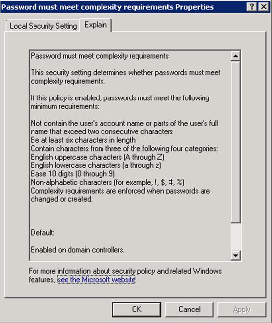
Figure 6.1: Password Security Setting Rules and Restrictions
H. Licensing ArcGIS Server on the Instance
As with the resetting of the instance password, these licensing steps need only be performed once after launching your instance.
- In preparation for completing the software authorization, go into the Lesson 6 module in Canvas and click on the Authorization file for ArcGIS Server link. This file has a .prvc file extension. You can download this authorization file on the instance or on your local machine.
- Run the Software Authorization for ArcGIS Server Authorization app on your instance (found in the ArcGIS folder on the Start menu).
- Select the I have received an authorization file... option, and click Browse. You should see drives from both your instance and your local machine.
- Locate where you stored the .prvc file you downloaded from Canvas, select it, then click Next.
- Select Authorize with Esri now using the Internet, and click Next.
- Accept the filled-in information (for one of the course authors/instructors), and click Next.
- Set Your Organization to Education/Student, Your Industry to Higher Education, Yourself to Student, and click Next.
- The Authorization Number should be filled in. Click Next.
- Authorization numbers may/may not also be filled in for several extensions. We won't need extensions for what we're doing in this class, so just click Next regardless.
- Leave the boxes for other extensions unchecked, and click Next.
- Click Finish.
I. Installing SQL Server Express on the instance
Esri supports the implementation of enterprise geodatabases using a number of relational database management packages (e.g., Oracle, SQL Server, Postgres). To expose you to another RDBMS that's commonly used in the industry, I'm going to ask you to install SQL Server Express. (This is a free, lite version of Microsoft's SQL Server package. For everything we'll do in this class, the two SQL Server packages operate the same.)
- In Canvas, download the SQL Server Express 2017 executable and copy it to your instance.
- Run the executable, choosing the Basic installation type.
After a few minutes, you should see that installation completed successfully. We'll also want to install SQL Server Management Studio, an app that's analogous to pgAdmin from earlier in the course. - Click the Install SSMS button at the bottom of the SQL Server Express installation dialog, which should open a page in your web browser.
- Locate and click on the Free Download for SQL Server Management Studio (SSMS) link.
- Run the SSMS installation executable, clicking Install on the resulting dialog.
With that, we're ready to begin playing with our enterprise geodatabases. First, you'll read a bit about ArcSDE, a technology that enables the ArcGIS products to work with data stored in an RDBMS.
What is ArcSDE?
What is ArcSDE?
ArcSDE is software that enables ArcGIS applications to store, manage and retrieve data in a RDBMS. The “Arc” comes from the ubiquitous naming convention used by Esri for their products. The SDE part stands for Spatial Database Engine.
ArcSDE is sometimes described as middleware, a layer of software that sits between Esri’s ArcGIS products and RDBMS software and manages data exchanges between them. It makes it possible for GIS data users to utilize their data without need for special knowledge of the underlying RDBMS.
As of ArcGIS 10, ArcSDE supports the commercial RDBMS’s Oracle, SQL Server, DB2, and Informix, and the free and open-source PostgreSQL.
In the last lesson, you worked with file geodatabases, a format that Esri recommends for small, single-user projects. Esri often refers to geodatabases stored in an RDBMS and accessed using ArcSDE as multiuser geodatabases because they are better able to support access by more than one user. The advantages of a multiuser geodatabase include:
- better data security through the granting of different levels of access to datasets to different users;
- backup and recovery capabilities;
- versioning which provides the mechanism for multiple users to access and edit data simultaneously;
- archiving which makes it possible to efficiently track changes made to datasets over time.
Esri enables users in the Amazon cloud to run ArcGIS Enterprise on either the Ubuntu operating system or Windows. While there would be some benefit to seeing how Postgres operates as an Esri enterprise geodatabase, we're going to proceed with SQL Server on Windows, as SQL Server is more commonly used in the industry as a geodatabase DBMS. That said, the concepts involved in administering an enterprise geodatabase are similar regardless of the RDBMS used, so what you learn here will be transferrable to other RDBMS’s.
One of the first things you might want to do after launching an enterprise geodatabase is set up login roles and privileges for those roles. That will be the focus of the next section of the lesson.
Adding Users and Data to Your Geodatabase
Adding Users and Data to Your Geodatabase
Logins and users in SQL Server
Before diving into enterprise geodatabase concepts, it's important to understand some basics of working with SQL Server, the DBMS that we'll be using on our Amazon cloud instances. (While we're actually using SQL Server Express, I will refer to the software as simply SQL Server, since the two operate essentially the same for our purposes in this class.) Access to SQL Server itself is granted through logins. A login allows someone to authenticate with SQL Server and answers the question, "Who is connecting?" Access to an individual database (of which there could be several for a given SQL Server instance) is granted through users. Whereas logins are concerned with authentication, user accounts provide authorization to perform different tasks with a database. They answer the question, "What can this person do in the database?" As we'll see, logins must be mapped to database user accounts in order to work with database objects. This blog post [50] provides further information.
Related to logins and users is the concept of roles. A role provides a way to group similar users together so that permissions can be granted more easily. Database administrators can define their own desired roles and make permission changes for those roles as they see fit. SQL Server also comes with a set of fixed server and database roles whose permissions cannot be changed. Among these is the sysadmin role, which, as you might guess, has permissions that grant full control over the server.
Geodatabase ownership
All databases found on a SQL Server instance have a special user called DBO (short for database owner). Any member of the sysadmin fixed server role who uses a database is mapped to the DBO user, and any object created by any member of the sysadmin fixed server role belongs to DBO automatically.
An important consideration when implementing an enterprise geodatabase in SQL Server is who will be the owner of the geodatabase -- the DBO user or the SDE user. While the DBO user is the person who administers the database at the SQL Server level (e.g., creating new users and roles), the SDE user is the person who administers the database within ArcGIS (e.g., updating database statistics and compressing the database). Esri's documentation includes a page that discusses the pros and cons of each [51] [https://pro.arcgis.com/en/pro-app/help/data/geodatabases/manage-sql-server/comparison-geodatabase-owners-sqlserver.htm]. Generally speaking, if the SQL Server database administrator and the geodatabase administrator are the same person, then having the DBO user own the geodatabase is sensible. If, on the other hand, those two roles are filled by different people, then having the SDE user own the geodatabase is probably more advisable. In this course, we're going to work with a DBO-owned geodatabase.
A reminder, if and when you restart your instance of the AMI
In the next section, you will be back working, via your Remote Desktop Connection, on your instance of the Amazon Machine Image (AMI) that holds our enterprise geodatabase, etc.
If you STOP-ed your instance on purpose, or if your Remote Desktop Connection gets interrupted, you will need to re-START your instance via the EC2 Console.
And, if the IP address of the machine you're connecting with has changed since your last connection, remember that you may need to edit the RDP rule to allow connection from your new IP address.
Changing authentication settings
Before we move on to setting up geodatabase users and roles, there are a couple of authentication settings we will change to make our lives a bit easier in this safe learning environment.
The first will be to set up SQL Server to allow mixed-mode authentication. By default, SQL Server only allows authentication through operating system logins. However, it is also possible to authenticate via user names and passwords stored in the database. In a real-world implementation, you may find it advantageous to utilize Windows authentication. But since that involves a bit of extra work on the instances we've just created, we'll go with SQL Server authentication.
The second setting we'll make will be to relax the default password standards on the Windows Server operating system that filter down to SQL Server. This will allow us to avoid the need to create lengthy, complex passwords.
- In your remote desktop window, launch the Microsoft SQL Server Management Studio. You should find it under Start > Microsoft SQL Server Tools.
(You might consider right-clicking on the Management Studio application and selecting Pin to Start and/or Pin to Taskbar for quicker access to it later.) - In the Connect to Server dialog that appears, enter LOCALHOST\SQLEXPRESS as the Server Name and click Connect.
- In the Object Explorer pane on the left side of the window, right-click on the LOCALHOST entry at the top of the tree and select Properties.
- Click on the Security page, then change the Server Authentication option from Windows Authentication mode to SQL Server and Windows Authentication mode. Click OK, and click OK to the note about needing to restart for changes to take effect.
- Right-click on the LOCALHOST server, and choose Restart.
- While the server is restarting, open the Server Manager (found under the Start menu).
- In the upper right of the Server Manager window, select Tools > Local Security Policy.
- Under Account Policies > Password Policy, double-click on Password must meet complexity requirements and choose Disabled. Click OK, and close both the Local Security Policy dialog and the Server Manager.
We'll now be able to authenticate using simple, easy-to-remember passwords. Obviously, in a real-world implementation, you would want to think twice before lessening your database security like this.
Create an Enterprise Geodatabase
Esri's ArcGIS Server/Enterprise AMIs have gone back and forth, sometimes including database software and a pre-configured enterprise geodatabase, sometimes not. This version's AMI does not -- we had to install the RDBMS ourselves -- so let's now create our first database.
- Return to SQL Server Management Studio, and Connect to the local server.
- Right-click on Databases, and select New Database.
- Set the Database name to egdb (short for enterprise geodatabase).
- Click OK to create the database.
At this point, this is an "ordinary" database. We'll next connect to the database in ArcCatalog, then use an Esri tool to turn it into a "geo" database.
Connect to the database as DBO
We'll start our work with the egdb database by connecting to it as the DBO user.
- On your remote connection desktop, open ArcGIS Pro if it's not open already. I suggest selecting Start without a template.
- In the Catalog pane, right-click on Databases, and select New Database Connection.
- Choose SQL Server as the Database Platform if it's not selected already.
Specify LOCALHOST\SQLEXPRESS as the Instance.
For Authentication type, select Operating system authentication. You'll see that there are no User name and Password fields as you would see if you had instead chosen Database authentication. This is because you'll be authenticating based on how you logged in to the current Windows Server session (in this case as the user Administrator who has system administrator privileges in both Windows and SQL Server).
Select egdb as the Database to connect to, and click OK. A new ready-to-be-named connection will appear under the Databases heading. The user making the connection and the geodatabase being connected to are important components of the connection, so I suggest including that information in the connection name. - Name your connection dbo_egdb.sde. The user is dbo and the database is egdb.
The egdb database is empty since you just created it, so you won't see anything listed in it yet.
Convert the database to a geodatabase
- Open the Geoprocessing pane (Analysis > Tools). (It may take a while for this to open the first time.)
- Click the Toolboxes heading, then expand Data Management Tools > Geodatabase Administration, and open the Enable Enterprise Geodatabase tool.
- Set the Input Database Connection parameter by clicking on the Browse button (folder icon) and selecting the dbo_egdb connection you just created.
- Set the Authorization File parameter by navigating to C:\Program Files\ESRI\License10.9\sysgen\keycodes. (Note: If you're unable to browse to this file, see the workaround described in this tech support article [52].)
- Click OK to execute the tool. If the tool executed successfully, the resulting dialog will tell you that it:
Created geodatabase tables and stored procedures.
Finished creating geodatabase schema.
Before adding some data to the geodatabase, let's discuss the importance of users and roles in a geodatabase context and lay out the scenario for the rest of our work in this section.
Users and roles in the geodatabase
Database roles enable the database administrator to improve security by assigning users or groups of users various levels of access to the database tables. Commonly used roles in an enterprise geodatabase include viewer, editor, etc. As the names of these roles imply, one user group might be limited to read-only access to data while another group might be allowed to both read and edit the data. While we're only getting to this topic now, you should keep in mind that similar strategies can also be applied to the kind of Postgres/PostGIS databases we talked about in previous lessons.
For illustration purposes, imagine you work in the U.S. federal government and that you are administering a geodatabase that will host data from a number of different departments: state boundaries from the Census Bureau, major highways from the Department of Transportation, rivers from the Department of the Interior, etc. You want each department to have stewardship over their data and to have just read-only access to other departments' data.
Click here to download to your machine the Lesson 6 data [53]. In the steps below, you will then copy said us_data.zip archive file from your local machine to your remote instance. The Downloads (or Documents) folder on your remote instance is a logical place to paste and unzip the data.
- Go to the taskbar on your remote desktop, and open the File Explorer (via the file-folders icon).
The File Explorer will open to the contents of This PC. In the Devices and drives list, you’ll see the drives that exist on your local computer and the drives that are on your remote instance. - Find the us_data.zip file that you just retrieved, and copy it to the Local Disk Downloads folder.
- Unzip the us_data.zip file that you just uploaded.
There are four Shapefile datasets.
Note that in our enterprise database environment, vector data is stored as feature classes. So, later, the Shapefile datasets that I gave you will be uploaded and converted to feature classes.
One aspect of the data loading/creation process that's worth keeping in mind is that when a feature class or feature dataset is created in the geodatabase, its name in the ArcGIS applications has two parts:
<owner>.<feature class/feature dataset>
Some organizations set up users specifically to handle data loading/data creation so that the owner listed in the two-part name clearly conveys the department that maintains the data. Following on this practice, let's add a user to the database who will control the loading of the Census data.
Add a data loader/creator to the geodatabase
The Create Database User tool is one of several geodatabase administration tools available through the ArcGIS Pro GUI.
- Again on your remote connection desktop, return to the geoprocessing Toolboxes.
- At the same Data Management Tools > Geodatabase Administration path, open the Create Database User tool.
In the Create Database User dialog, set the Input Database Connection field to your dbo_egdb.sde connection.
We're going to use database authentication for this user, so leave the Create Operating System Authentication User box unchecked.
Enter a Database User name of census.
To make this easy to remember, enter the same string (census) for the Database User Password.
Leave the Role field empty. We'll discuss roles shortly, but you should note that if any database roles existed, you would have the option of associating the new user with a role in this dialog.
Click Run to create the new user.
With the new user created, let's add a database connection based on that user's authentication parameters. - As you did earlier, access the New Database Connection dialog.
The Database Platform and Instance should be correctly specified as SQL Server and LOCALHOST\SQLEXPRESS already.
Change the Authentication Type to Database authentication.
Enter the census:census User name and Password combination established above.
You will probably want to leave the Save user name and password box checked for your work here, though this is another setting you'd want to consider carefully in a real-world implementation.
If you entered the name and password properly, you should be able to select egdb from the Database dropdown.
Click OK to create the connection. - Following on the convention suggested earlier, rename the connection to census_egdb.sde.
Loading data
With the census user created, let's work as that user to load the state and city data you downloaded above. Because feature datasets are frequently used to house feature classes, let's create one of those first.
- Right-click on the census_egdb.sde connection, and select New > Feature Dataset.
- The Output Geodatabase parameter should be filled automatically with the census_egdb.sde connection, so leave that setting in place.
- Set the Feature Dataset Name to usa.
- The data you'll be importing are in geographic coordinates, NAD83 datum, so specify that as the Coordinate System for this feature dataset, and click Run.
You should see a new CENSUS.usa feature dataset appear under your connection. - In the Catalog pane, right-click on Folders, select Add Folder Connection, and make a connection to the folder where you copied the data (if the Downloads folder, you'll need to navigate to C:/Users/Administrator/Downloads).
- Now, expand the census_egdb.sde connection, and right-click on the CENSUS.usa feature dataset, and select Import > Feature Class(es).
Setting the Input Features parameter, browse to where you unzipped the us_data shapefiles, and select the us_boundaries and us_cities shapefiles.
Confirm that the Output Geodatabase is set to your CENSUS.usa feature dataset and click Run.
After a few moments, new CENSUS.us_boundaries and CENSUS.us_cities feature classes should appear in the CENSUS.usa feature dataset. - For additional practice, repeat the steps above to create a new transportation user, connect as that user, and load the us_roads shapefile into the geodatabase.
An important point to note about the process we just went through is that users created via the Create Database User tool have the ability to load/create data. It's generally considered a best practice to restrict this ability to a small number of trusted administrators to avoid cluttering the database with unwanted data. We'll now see that following this best practice requires adding lower-permission users through a different process.
Adding data editors/viewers to the geodatabase
Returning to our scenario, the users in the departments are as follows:
| Department | editors | viewers |
|---|---|---|
| Census | Moe | Larry, Curly |
| Transportation | Lisa | Bart, Homer |
| Interior | Stan | Cartman, Kenny |
To add these users, we'll need to return to the SQL Server Management Studio.
- If you closed your Management Studio window earlier, re-open it and connect to LOCALHOST\SQLEXPRESS using Windows Authentication.
- In the Object Explorer, expand the Security folder, then right-click on Logins and select New Login.
- In the Login – New dialog, enter a Login name of Moe.
Select SQL Server Authentication, then a Password of Moe (it's case-sensitive, same as the login name).
Uncheck each of the three checkboxes (Enforce password policy, Enforce password expiration, User must change password at next login). Again, this is a place where you might choose differently in a real-world implementation.
Set the Default database to egdb.
Click OK to create the new login. - If you expand the Logins folder, you should now see a Moe login, along with census and transportation, which were created by the ArcGIS Add User tool earlier.
We'll now associate the new login with the egdb database that you created above. - In the Object Explorer, navigate through the following folders: Databases > egdb > Security > Users. Again, you should see census and transportation here, listed as users in the egdb database.
- Right-click the Users folder and click New User. In the Database User – New dialog:
Enter a User name of Moe.
Enter a matching Login name of Moe. (You could also click the '...' button to the right to browse the list of logins associated with the SQL Server instance.)
Important: Leave the Default schema blank. If you wanted Moe to have the ability to own data in the geodatabase (i.e., to create new feature classes), then you would enter Moe as the default schema. The ArcGIS Create Database User tool makes this setting for the new user, which is why we're not using that tool to create lower-level users like Moe, but instead using SQL Server Management Studio as outlined here. The reasoning behind the different user creation process is found in Esri's documentation [54]:
"Users who own data must also have schemas in the database that have the same name as the user name."
Click OK. Moe should now have access to the egdb database. - Return to ArcGIS Pro and establish a database connection for user Moe following the steps used to create the census_egdb connection earlier.
Note: At this point, you're emulating what a non-administrative user of your database would go through to connect to the geodatabase. Earlier connections and data loading procedures are tasks that you would be more likely to carry out in a database administrator role.
After creating a connection for Moe and opening that connection, you'll find that Moe is not able to see any of the data that's been loaded into the database. We'll look at how to fix that shortly. - Repeat the steps above to add Larry and Curly (and Lisa, Bart, and Homer if you're so inclined) as egdb geodatabase users.
Creating roles
In order for users to have the ability to view and/or edit the data in a geodatabase, the data owner must grant those privileges. That can be done on a user basis (using an ArcGIS tool), but the process can be done more efficiently by assigning users to roles and assigning privileges to the roles. In this section, you'll create a viewer role and an editor role in the egdb database.
One important note on roles: while the privileges must be granted by the data owner (the census and transportation users in our scenario), the roles must be created by someone with sysadmin privileges. That is the DBO user in our implementation.
- Return to the Geoprocessing pane > Toolboxes > Data Management > Geodatabase Administration. Open the Create Role tool.
- In the resulting dialog, set the Input Database Connection parameter to your dbo_egdb.sde connection.
- For Role, enter viewer.
- Confirm that Grant role (and not Revoke role) is selected in the next dropdown.
- In the User Name(s) field, enter a list of the users you created in the section above who were listed as viewers. As it says in the Tool Help panel, the user list should be separated by commas (no spaces).
- Click Run.
- Repeat these steps to create an editor role for the appropriate users.
If you're paying close attention to the scenario, you might be thinking we should have separate editor roles for each of the three data owners, such that Moe can only edit his Census data, Lisa can only edit her Transportation data, and Stan can only edit his Interior data. You're welcome to implement that sort of design if you wish, but for simplicity's sake, feel free to create just a single editor role.
Manage geodatabase privileges
Finally, we'll now work through the data owner connections to assign the proper privileges to go with the roles just created.
- Return to the Geodatabase Administration toolbox and open the Change Privileges tool.
- For the Input Dataset parameter, browse to the CENSUS.usa feature dataset (through either the census or dbo connection).
- The User parameter can be set to either a user or a role. We want to set the viewer role's privileges here, so enter viewer for this parameter.
- For the View parameter, select the Grant view privileges option.
- For the Edit parameter, confirm that the Do not change edit privileges option is selected.
Since you learned about SQL earlier in the course, it should make sense that the View privilege has Select next to it in parentheses and that the Edit privilege has Update/Insert/Delete next to it. - Click Run to apply the changes. This will provide the same level of privileges across all feature classes housed within the usa feature dataset.
- Repeat these steps to assign both View and Edit privileges to the editor role and, if desired, repeat the process for the data owned by the transportation user.
- Now, in a map, test the settings you've made by making database connections through at least Larry and Moe and attempting to perform some edits (such as creating a new state and/or deleting an existing one). For example:
- Larry should be able to view all feature classes, but not edit them.
- Moe should be able to both view and edit all feature classes.
- Neither Larry nor Moe should be able to import or create a new feature class.
(Hint: you make Database Connections via the Catalog pane.)
Note:
- Privileges can be assigned at the feature class level, but only if the feature class is not part of a feature dataset. When dealing with a feature dataset, privileges must be assigned at the dataset level (as outlined above), and they will cascade to each child feature class.
- The Input Dataset parameter supports specifying multiple datasets/feature classes at once.
- It is also possible to right-click on a feature dataset/feature class and select Manage > Privileges.
This concludes the hands-on activities you'll be doing with your geodatabase instance in this lesson. Feel free to do some experimenting with your instance. When done, close the remote desktop connection to your instance, and most importantly, remember to stop your instance through the EC2 Console to avoid racking up unnecessary charges.
Go on to the next page to see this week's graded activity.
With that, we've finished our tutorial on creating a SQL Server geodatabase, adding users, loading some data, and assigning data privileges to the users. You weren't specifically instructed to add the Department of the Interior users and import the us_hydro shapefile, but you're welcome to do so if you're looking for additional practice.
Project 6: Describe the Data Users in Your Organization
Project 6: Describe the Data Users in Your Organization
A. Assignment description
In the Adding Users and Data to Your Geodatabase part of the lesson, it discusses the various 'roles' that people who are involved with an enterprise geodatabase might have.
For Project 6, I'd like you to spend some time reflecting on the data users in your organization. If you already utilize an enterprise geodatabase, tell me a bit about your system, who uses it, through what login roles, and with what privileges. In preparation for this write-up, you may want to talk to your geodatabase administrator if that person is not you.
If your organization isn't using an enterprise geodatabase, tell me a bit about your data workflows and users, and spend some time describing the login roles and privileges you think would best meet your organization's needs if you were to implement one.
It's not necessary for you to divulge the identities of co-workers, but you may find that your write-up flows better if you use at least first names. You can always use fictitious names if you have concerns about identifying people by their real names.
Some of the job responsibilities frequently associated with geodatabase usage that you may want to consider include:
- database administration (at the RDBMS level)
- database administration (at the ArcSDE level)
- database design
- data ownership
- data QA/QC
- data editing
- map production
- GIS analysis
Note: If you feel you're unable to report on a current or former workplace, I will also accept an analysis of any organization that has published information on its enterprise geodatabase implementation. Such reports can be found by doing an online search for GIS + "master plan" or "strategic plan."
B. Deliverables
This project is one week in length. Please refer to the Canvas Calendar for the due date.
- Submit your analysis of your organization in Word or PDF format to Lesson 6. The length of the write-up should be at least one page single-spaced. Your submission will be graded as follows:
- Quality of analysis (the extent to which you demonstrate a thoughtful evaluation): 70 of 100 points
- Quality of write-up (in terms of grammar, spelling, flow): 30 of 100 points
- Complete the Lesson 6 quiz.
Lesson 7: Data Management in an Enterprise Geodatabase
Overview
Overview
Now that you've gotten your feet wet with an enterprise geodatabase, it's time to dig into some of the details of managing vector and raster data in that environment. In this lesson, you'll learn how to add new feature classes and raster data sets to an enterprise geodatabase and about steps that should be taken after the creation of new datasets. You'll also see how geodatabase data is stored within SQL Server.
Questions?
If you have any questions now or at any point during this week, please feel free to post them to the Lesson 7 Discussion Forum.
Checklist
Checklist
Lesson 7 is one week in length. See the Canvas Calendar for specific due dates. To finish this lesson, you must complete the activities listed below. You may find it useful to print this page out first so that you can follow along with the directions.
- Download a .zip archive containing four shapefile datasets that we used back in Lesson 3 and in Project 4. DataFromLessons3and4.zip [55]
- Download some new data that you'll need for Lesson 7. Lesson7_data.zip [56].
- Work through Lesson 7.
- Complete the Charlottesville historical geodatabase compilation project and write-up described on the last page of the lesson.
- Take Quiz 7.
Feature Class Creation: Via Import
Feature Class Creation: Via Import
In the previous lesson, we saw how to import vector data into new geodatabase feature classes as part of our experimentation of logins, users and roles. Most of this section of Lesson 7 will be reviewed as we import more data, though the process is outlined in greater detail here.
A. Transferring data from your computer to your enterprise geodatabase instance
We are going to transfer four shapefile datasets from your computer to your Amazon cloud enterprise geodatabase instance. The shapefiles are data you worked with back in Lessons 3 and 4: the States, counties, and us_cities shapefiles that we used in Lesson 3, and also the cities shapefile that you used in Project 4 in the Jen and Berry's site selection exercise. I gave you copies of them in the DataFromLessons3and4.zip archive that you downloaded in the Checklist section, above.
- Restart your instance.
You are next going to open a Remote Desktop Connection to your geodatabase instance. If you allocated an Elastic IP for your instance as instructed in Lesson 6, then you can connect using that same address. Otherwise, you'll need to connect using the new Public IP assigned to your re-started instance.
Also, if the IP address you're connecting from has changed, then you'll need to refresh the RDP Security setting by going to your instance's security group and updating the Inbound RDP rule. - Open a Remote Desktop Connection to your geodatabase instance through the appropriate IP address.
- In doing so, make certain that the box for Drives is checked via Options > Local Resources > More button.
- In your remote desktop connection window, open Windows Explorer (This OS version calls it File Explorer). There should be an icon for it on the taskbar along the bottom of the remote connection window. If not, wend your way via the Start button to it.
Click This PC to display the drives that are attached to the Windows operating system.
Under Devices and drives, you will see listed a set of drives (Local Disk C and possibly also Local Disk D) for your EC2 instance.
You will also see the drives that reside on the computer you are remote-connecting from. They will have names like C on <the name of your computer>.
In the next steps, you are going to Copy-Paste the files making up the four shapefiles from your computer to the Local Disk (C:) drive on your instance.
So, you might want to open a second File Explorer window.
To open another File Explorer window, right-click on the File Explorer icon on the taskbar, and choose File Explorer. - Copy the DataFromLessons3and4.zip archive from your local machine to the virtual machine in your remote instance.
- Browse to the folder on your local computer that contains the DataFromLessons3and4.zip archive.
Highlight it, and click Copy. - Now (via your second File Explorer window), navigate into the Local Disk (C:) drive on your remote desktop connection. Create a new folder named data on the C: drive.
Browse to within the data folder, and Paste the shapefile zip archive file there.
The copy/paste process may take several seconds.
- Browse to the folder on your local computer that contains the DataFromLessons3and4.zip archive.
- Un-zip the DataFromLessons3and4.zip archive.
Leave the uncompressed file destination the name of the zip archive: DataFromLessons3and4, so that the data ends up in a folder by that name. - In your remote connection, you may choose to open your ArcGIS Pro project from Lesson 6 to re-use the Folder connection to the Local Disk (C:) drive. Otherwise, you can re-create it in a new project.
- Expand the folder connection to the C:\ drive, and make certain that in your DataFromLessons3and4 folder you have four shapefile datasets — States, counties, and us_cities from Lesson 3, and cities from Project 4.
To learn more about issues concerning moving data into the cloud, go to the Moving data to the cloud [57] section of our Cloud and Server GIS course, and read from the beginning of that section through the Techniques for data transfer subsection.
B. Importing to your database from a shapefile or file/personal geodatabase
A common workflow for organizations that are migrating their data to an enterprise geodatabase is to import data that already exist in other formats. Let's walk through that process.
- You should already have opened ArcGIS Pro. In the Catalog pane, you should have some connections under the Databases heading left over from the previous lesson, including:
dbo_egdb
census_egdb
transportation_egdb
Recall that the latter two connections were through database users we created for the specific purpose of loading data.
We're going to import the States, counties, and us_cities shapefiles as feature classes.
We'll first create a feature dataset to house the new feature classes. - Right-click on the census_egdb.sde connection heading, and select New > Feature Dataset.
- Assign a name of usa_L7.
- For the Coordinate System parameter, perhaps the easiest way to set it is to import the coordinate system definition from one of the feature classes you plan to house in the dataset.
- Click the globe icon to open the Coordinate System dialog. Select Import Coordinate System from the Add Coordinate System dropdown list on the right side of the dialog (
 ), then browse to and select the C:\data\DataFromLessons3and4 States shapefile and click OK.
Click OK again to dismiss the Coordinate System dialog.
After a few moments, you should see the new usa_L7 feature dataset listed beneath your census_egdb connection. Note that the full name listed in the Catalog window is egdb.CENSUS.usa_L7, indicating that census is the owner of the feature dataset. - Right-click on the usa_L7 feature dataset, and select Import > Feature Class. We'll use the multiple feature class option in a moment. The single option provides slightly different functionality.
- For the Input Features browse to the location of the States shapefile.
The Output Location should already be filled in with the usa_L7 feature dataset accessed through the census_egdb connection. - For the Output Feature Class, assign the name states.
Though we won't use them, the next two optional settings are worth a brief mention. The first, Expression, allows for specifying a subset of the input dataset to import through an SQL Where clause. The second, Field Map, allows for some control over the fields that will be imported to the GDB feature class. For example, you might choose not to import certain fields. The Field Map parameter also makes it possible to produce an output field based on values from multiple input fields (e.g., the concatenation of two text values or the sum of two numeric values). - Click Run to begin the import process. After a few moments, you should see the states feature class listed in the Catalog pane and added to the map.
Now, let's use the multiple feature class import option to import the counties and us_cities shapefiles. - Right-click on the usa_L7 feature dataset, and select Import > Feature Class(es). As the name implies, this tool makes it possible to import a list of shapefiles, coverages, or feature classes. It doesn't provide the flexibility of importing a subset of records or customizing the output fields, so you'd use this tool only if you have no need for those options.
- For the Input Features, browse to and select the counties and us_cities shapefiles – you can hold the Ctrl key to select them both at the same time..
The Output Geodatabase should already be defined correctly, as your usa_L7 feature dataset. - Click Run to begin the import process.
This import is likely to take a bit of time because of the volume of vertices in the counties shapefile.
Unlike the single feature class tool, it will not automatically add the new feature classes to the map.
Also, because you already added a us_cities feature class in Lesson 6, ‘_1’ will be added to the us_cities feature class you're importing now. Regardless of the fact that this feature class is in a different feature dataset, it is being stored as a table in the same SQL Server schema, so it must have a different name.
Of course, it's also possible to import stand-alone (non-spatial) attribute data tables to your geodatabase. We didn't see options for that above because we had right-clicked on a feature dataset, which is designed to store only feature classes (tables with geometry). - Right-click on your census_egdb connection (made back in Lesson 6), and hover your mouse over the Import menu. You should now see options for importing a single or multiple tables.
Recall from the last lesson that users created using the Create Database User tool are able to load data and create new feature classes from scratch, and that it's considered a best practice to limit these capabilities to administrative staff. We used SQL Server Management Studio to create users who we didn't want to grant data loading ability.
Speaking of creating new tables from scratch, let's take a look at that workflow in the next section.
Always remember to Stop your EC2 Instance when you finish or when you take a long break.
Feature Class Creation: From Scratch
Feature Class Creation: From Scratch
In this section of the lesson, we'll look at creating a new feature class and populating it using the Append tool. To illustrate the process, imagine you're again working for Jen and Barry.
A. Create a new data loader
- Have your enterprise geodatabase instance running and be connected to it via remote desktop connection.
- Open ArcGIS Pro.
We're going to create a new user (jb) to be the data owner for the Jen and Barry's data (that we borrowed from Lesson 3). - Open the Create Database User tool that we used in Lesson 6 (Analysis > Tools > Data Management > Geodatabase Administration).
- Set the Input Database Connection parameter to your dbo_egdb.sde connection.
As we did in the last lesson, leave the Create Operating System Authenticated User box unchecked.
Set the Database User and Database User Password to jb.
Set the Role to editor. (Recall that we created this role last week.)
Click Run.
- Now, use New Database Connection to create a connection to the egdb database through the new jb user. Name the connection jb_egdb.
B. Create a new empty feature class
- Access your new jb_egdb connection.
- Create a new feature dataset called pa (for Jen and Barry's Pennsylvania data).
Import the coordinate system definition from the Jen and Barry's cities shapefile. - Right-click on the pa feature dataset, and select New > Feature Class. You now need to work through a multi-panel dialog.
Assign a name of cities to the feature class.
Set its feature type to Point Features, and click Next to move on to the next panel. - In the Fields panel of the dialog, add the following fields to the feature class:
cities feature Class Fields Name data type population Long Integer total_crim Long Integer crime_inde Double university Short Integer - We'll be accepting the default values for the rest of the settings. You can have a look at the other settings by clicking Next or you can click the Finish button.
New features can be added to the feature class using Pro's editing tools, which were covered in detail in GEOG 484. Another way to populate a feature class is by using the Append tool.
C. Load data with the Append tool
As its name implies, the Append tool is used to append features held in feature classes/shapefiles to another existing feature class. Let's use it to append the features in our Jen and Barry's cities shapefile to the empty cities feature class we just added to our geodatabase.
- Open the Geoprocessing pane.
- Open the Append tool found at Data Management Tools > General > Append.
For Input Datasets, browse to your Jen and Barry's cities shapefile. (In the DataFromLesson3and4 folder.)
For Target Dataset, browse to your egdb.JB.cities feature class. (In the egdb database.)
The next part of the dialog is concerned with whether the fields in the input dataset match the fields in the target dataset. The default must match option checks to see if the fields match (in name and data type) and will not allow the append operation to occur if there is a mismatch. The Use the field map option allows for differences between the datasets.
Because our cities feature class doesn't have all of the fields found in the cities shapefile, select the Use the field map option.
Note that the four fields we defined above when creating the feature class are listed under the Output Fields heading. For each field, we have the ability to, as mentioned on the previous page, populate it in advanced ways, such as by concatenating values from multiple source fields or by summing values from multiple source fields. We're just going to do a straight 1:1 transfer of values, so you can leave the default Field Map settings in place.
Click Run to carry out the append operation.
Points should appear on the map, and of course, the attribute table of the egdb.JB.cities feature class will become populated with data.
A couple of notes on the Append tool that you should keep in mind:
- You're not limited to using this tool to populate a new empty feature class, as we did here. Features can be appended to any existing feature class.
- The real power in the Append tool which we didn't see here is that it allows for the selection of multiple input datasets. So if you had a number of similar shapefiles (e.g., census tracts for three states in three separate shapefiles), you could use the tool to combine all of the features into one feature class.
Always remember to Stop your Instance when you finish or when you take a long break.
After Loading Data
After Loading Data
Esri recommends the following after loading data into a geodatabase feature class:
- Calculate database statistics using the Analyze tool.
- Grant privileges for other users to access the data.
- Update metadata.
- Add geodatabase behavior (domains, sub-types, topology rules, etc.).
The second item above, which we covered last lesson, is the only one that is absolutely critical. The first item, which we'll discuss in a moment, can greatly improve performance, especially as the size of the feature class increases. Metadata, covered in GEOG 484 is often overlooked, but can save a lot of headaches for anyone who has questions about the data. Geodatabase behavior functionality, covered in GEOG 484 and in Lesson 5 in this course, offers useful ways to improve the efficiency and accuracy of data maintenance workflows.
To this list, I would add the implementation of attribute and spatial indexes to improve performance. This page of the lesson will focus on database statistics and indexes.
A. Calculating DBMS statistics using the Analyze tool
Relational database packages like SQL Server provide users with the ability to calculate basic statistics on their tables, such as the common values and data distribution in each column. These statistics are stored in system tables that are utilized by the DBMS to determine the best way to carry out queries, thereby improving performance. As a table's data changes over time, the statistics will become out of date and less helpful in optimizing performance. This is why Esri recommends running the Analyze tool after major edits are made to a feature class. Let's run the tool on the states feature class we imported earlier.
- In the Geoprocessing pane, open the Analyze Datasets tool.
- For the Input Database Connection, browse to Databases > census_egdb.sde and click OK. Note that tables can only be analyzed by their owner.
- The Datasets to Analyze box should fill with a list of datasets (in this case all feature classes) owned by the user associated with the connection.
Click Select All.
At the bottom of the dialog are checkboxes that control which tables associated with the selected datasets should be analyzed (base, delta and/or archive). The base table (sometimes referred to as the business table) is essentially what you see when you open the feature class's attribute table. The delta table stores changes made to the base data in a versioned feature class, while the archive table stores data enabling database users to retrieve historical states of a feature class. We'll look at these topics in the next lesson. For now, you can just leave all three boxes checked. No harm is done if the feature classes don't have delta or archive tables.
Click Run to execute the tool.
After a couple of seconds, the process will be complete. Close the Analyze Datasets processing window.
Keep in mind that running Analyze may have no perceptible effect for small datasets like we're dealing with here, but might result in significant performance gains in larger datasets.
B. Attribute indexes
Attribute indexes are another mechanism used in relational databases to improve performance, particularly in the execution of queries. Developing better indexing algorithms is one of the more popular research topics in the computer science field. A comprehensive review of indexing schemes is outside the scope of this course. But at the very least, you should understand that one of the more common schemes works much like the index of a book.
If you're looking for discussion of a particular topic in a book, you don't skim through each page of the book beginning with page one. You look up the topic in the index, which tells you the pages where you can conduct a much narrower search for your topic. A database index often works in much the same way. Given a WHERE clause like "WHERE city = 'Philadelphia'", the index helps the DBMS begin its search at a particular row of the table rather than at row one.
Some points to keep in mind regarding indexes:
- They can be based on one or more columns.
- They must be created by the table owner.
- The degree to which an index will help performance depends on the degree of uniqueness in the values being indexed. Highly unique column content will benefit most from an index, less unique column content will benefit less.
- They require a greater amount of disk space since they are essentially alternate representations of the data that must be stored and consulted by the DBMS.
- They can increase the processing time required for table edits since the DBMS needs to not only perform the edit but also update the index. For this reason, Esri recommends dropping indexes prior to performing bulk edits, then re-creating the indexes after the edits are complete.
To see how attribute indexes are built in ArcGIS, let's create one on the name column in the us_cities feature class.
- In ArcGIS Pro's Catalog pane, expand the usa_L7 feature dataset.
- Right-click on the us_cities feature class, and select Properties.
(Recall that the import process may have added a “_1” to the feature class name.) - In the Feature Class Properties dialog, click on the Indexes tab. Note that an index already exists on the OBJECTID field.
- In the Attribute Indexes section of the dialog, click the Add button.
- In the Fields available list, of the Add Attribute Index dialog, highlight the NAME column, and click the right arrow to copy it over to the Fields Selected list.
Leave the Unique checkbox unchecked. Checking this box specifies that the database can stop searching after the first match is found. Thus, you'd only want to check this box if each value in the index column appears only once. That would be a bad idea in this case, since some of the city names are duplicated.
But, do check the Ascending box. This will create an index in which the city names are sorted in ascending order.
Assign a Name of us_cities_name_idx.
Click OK to create the index. - Click OK again to dismiss the Properties dialog.
I won't bother to have you do a test query before and after because I doubt we'd see much difference in performance with such a small table. Just keep this capability in mind if you find that your queries are taking a long time to execute.
C. Spatial indexes
While attribute indexes improve the performance of attribute queries, spatial indexes are used to improve the performance of spatial queries. Esri geodatabases support three different methods of spatial indexing, grid, R-tree, and B-tree. The grid method is analogous to the map index found in road atlases. A grid of equal-sized cells is laid over the feature class, and each row and column of the grid is assigned an identifier. Geometries in the feature class are compared to this grid and a list of grid cells intersected by each geometry is produced. These geometry-grid cell intersections are stored in a table. In the example below, feature 101 intersects three grid cells, while feature 102 is completely within a single cell.
| FID | GX | GY |
|---|---|---|
| 101 | 5 | 9 |
| 101 | 5 | 10 |
| 101 | 6 | 9 |
| 102 | 4 | 8 |
Index tables like this are used to enable GIS software to answer spatial questions without having to look at each geometry in the feature class. For example, imagine selecting features from our us_cities feature class that are within the state of Pennsylvania. The software will first look up the grid cells intersected by Pennsylvania. It can then throw out all of the us_cities points that don't intersect those same grid cells. It only needs to test for containment on points that share grid cells with the Pennsylvania polygon. This testing of only the close features is much more efficient than testing all features.
It is possible to define up to three of these spatial grids per feature class. Multiple grids with different resolutions can capture the extent of features more efficiently especially when the feature class contains features that vary greatly in their extent (i.e., some small features and some large).
The grid method is employed by Esri file geodatabases and Oracle-based ArcSDE geodatabases that store geometry using the Esri ST_Geometry type. ArcGIS calculates a default grid that typically provides a high level of performance. This page in the Esri documentation (An overview of spatial indexes in the geodatabase) [58] provides further information on spatial indexes, including when you might want to rebuild one.
SQL Server geodatabase adminstrators have two options available for storing geometries: the Microsoft geometry and Microsoft geography data types, which are similar in concept to the geometry and geography spatial data types we saw in PostGIS. The default storage method when using SQL Server is Microsoft geometry. (More on how spatial indexing works for geometry and geography types can be found below.) This can be changed when creating a feature class by selecting Use configuration keyword on the last panel of the New Feature Class wizard. For example, if you have data covering a large spatial extent and want to use SQL Server's spatial functions to calculate spherical lengths and areas on the SQL command line, then storing the data using the geography type might be the way to go. Further information on these storage options can be found in the documentation (Configuration keywords for enterprise geodatabases) [59].
Another spatial indexing method employed in ArcGIS is the R-tree, which uses a set of irregularly sized rectangles (R stands for rectangle) to group together nearby objects. This (File: R-tree.svg) figure [60] helps to illustrate how an R-tree works. The red rectangles (labeled R8-R19) are the bounding boxes around some set of features (lines or polygons). The blue rectangles (R3-R7) are an aggregation of those features into groups, and the black rectangles (R1-R2) are a higher level of aggregation.
The basic idea of a search is the same, if the search geometry falls within R1 then the software knows it can disregard the features within the bounding boxes R15-R19 and instead focus on R8-R14. After that first check is completed, the blue level of the tree might be used to further narrow the search.
R-tree indexes are used in Oracle geodatabases that utilize the SDO_Geometry type. They are automatically created and managed by ArcGIS and while it is possible to delete and re-create an R-tree index, it's not clear that doing so would improve performance. If you're having performance issues in a geodatabase that uses R-tree indexing, you may want to dig further into the documentation and/or contact Esri customer support.
SQL Server-based geodatabases that implement the geometry or geography spatial type are spatially indexed using a B-tree method [61]. (As noted above, the geometry spatial type is the default in SQL Server.) This is an indexing method commonly used for non-spatial data, but in this context modified by Microsoft to handle spatial indexing as well. Like the R-tree method, this modified B-tree method employs a rectangular grid for locating features.
Finally, Postgres-based geodatabases are spatially indexed using a Generalized Search Tree (GiST) approach [62]. This indexing method was developed as an alternative to the older B-tree and R-tree methods for irregular data structures (such as GIS data). It realizes performance gains by breaking data up into groupings, like objects that are within, objects that overlap, objects to one side, etc.
Now that you've learned about some of the settings to consider when loading data into an enterprise geodatabase, let's look in SQL Server Management Studio to see how feature classes are stored. Reminder: remember to Stop your Instances when you finish or when you take a long break.
Looking Under the Hood of a SQL Server Geodatabase
Looking Under the Hood of a SQL Server Geodatabase
A. Feature class storage in SQL Server
Let's take a look at how the data we've been working with in ArcGIS Pro is stored in SQL Server.
- If you need to, log in to your enterprise geodatabase instance using Windows Remote Desktop.
- If you are still in the remote connection used for the earlier parts of the lesson, close ArcGIS Pro and open SQL Server Management Studio.
- Connect to the localhost server, and browse inside the egdb database (Databases > egdb).
- Expand the Tables folder, and note that all of the tables we've worked with in the last couple of lessons are found here (along with many others, some of which we'll discuss momentarily).
- Open the jb.CITIES table (right-click > Select Top 1000 Rows). Under the Results tab, you should see all of the attribute data along with a SHAPE column. Keep in mind that the values in the shape column are in Microsoft geometry format. You could work with your data using raw SQL much like we did with PostGIS by taking advantage of SQL Server's spatial data tools [63] [https://docs.microsoft.com/en-us/sql/relational-databases/spatial/spatial-data-sql-server].
- Close the CITIES table.
But in the Object Explorer pane, keep the list of Tables expanded.
B. Repository tables
ArcSDE relies on a number of tables behind the scenes. Many of these so-called repository tables are owned by the dbo superuser.
- Looking at the Tables listing, you should see a few "GDB_*" tables and many "SDE_*" tables. It's not important for you to know the purpose of all of these tables, but there are a few that are worth discussing.
The SDE_layers table stores information on all of the geodatabase's feature classes, which can be displayed as layers. - Open the dbo.SDE_layers table. The first column (layer_id) stores a unique ID for each feature class.
- Close the SDE_layers table.
You may notice a number of "i" tables. These tables help ArcGIS keep track of the next unique identifier available in each table. There is one "i" table for each feature class. The relationship between the "i" tables and their associated feature classes can be found in SDE_table_registry. - Open the SDE_table_registry table. The registration_id value is the linkage between the feature class and its "i" table. You might open up one of the "i" tables and note that the base_id indicates the next ID to be used in the event a new feature is added.
- Close the SDE_table_registry table.
Finally, it's worth pointing out that the "GDB_*" tables are where geodatabase behavior information is stored. For example, you can see the relationship between feature classes and their parent feature datasets in these tables. - Open the GDB_items table. Locate the row with a Name value of egdb.CENSUS.usa_L7, and make note of its UUID value. On my instance, its UUID is "{D7034507-7188-467F-BFB1-41F1F3FE2F3D}", but it will be different on your instance.
- Now, open the GDB_itemrelationships table. You should see that same value appear three times in the OriginID column.
The DestID values for those rows correspond to the UUID values of the egdb.CENSUS.us_cities, egdb.CENSUS.states and egdb.CENSUS.counties feature classes found in the GDB_items table.
It's not really important that you remember much about these repository tables. However, hopefully, you now have a bit of an appreciation for what's going on behind the scenes and will see the tables as a bit less of a mystery.
Always remember to Stop your Instance when you finish or when you take a long break.
Raster Management
Raster Management
Esri offers a number of different options for managing raster data in an enterprise geodatabase. One area that receives a good deal of attention is managing collections of adjacent raster data sets (e.g., aerial photos). The options for dealing with such collections range from working with the raster data sets individually to merging them together into one large data set. In between is something Esri calls a mosaic dataset which attempts to provide the best of both worlds, the ability to work with multiple raster data sets as one combined layer or to break them up into their individual components. We'll talk about a couple of these approaches in this section of the lesson.
A. Raster datasets
Let's see how to bring a raster data set into a geodatabase.
- Download this zipped raster image of the earth at night [64].
- Open a Windows Remote Desktop Connection to your enterprise geodatabase instance if you haven't already.
- Copy the earthatnight.zip file to the C:\data folder on your remote instance and unzip it.
- Open ArcGIS Pro and open the Geoprocessing pane.
- Open the Raster to Geodatabase tool (Conversion Tools > To Geodatabase).
- For the top Input Rasters parameter, browse to your C:\data folder and select your earthatnight.bil raster.
- For the Output Geodatabase parameter, browse to one of your data loading users (e.g., dbo_egdb.sde).
- Click Run to begin the import.
- After the import has completed, refresh the connection's listing if necessary, and add the raster to a map to confirm that it imported properly.
Now, let's take a moment to look at how the imported earthatnight raster looks from within SQL Server.
- Close ArcMap and open SQL Server Management Studio (SSMS).
- In SSMS, browse to Databases > egdb > Tables.
- Open the EARTHATNIGHT table, and note that it contains just one row. This table doesn't store the raster data itself, but rather the footprint of the raster (a polygon representing the area that it covers). Other information associated with the raster can be found in the following supporting tables:
- SDE_blk_1: pixel data
- SDE_bnd_1: metadata on the raster's bands
- SDE_aux_1: statistics (similar to those used to improve vector dataset performance) and color maps
The "_1" part of these table names comes from the rastercolumn_id value assigned to the raster, found in the SDE_raster_columns repository table. If the earthatnight raster instead had a rastercolumn_id of 2, its pixel data would be stored in SDE_blk_2, for example.
Raster datasets can hold either integer or floating-point data. They can also be comprised of multiple bands. If you have a single-band integer raster dataset, a value attribute table (VAT) can be built that stores the number of cells associated with each integer value. The earthatnight raster holds integer values, but it is comprised of three bands. If it were a single-band integer raster dataset, we would see an SDE_vat_1 table in addition to the other tables.
B. Mosaic datasets
As mentioned at the beginning of this section, it is common in GIS to deal with collections of adjacent raster datasets. Esri's mosaic dataset can be used to treat such collections as a single unit while still having the ability to work with the individual files as needed. Let's create a mosaic dataset to manage some elevation raster data sets for the State College, PA, area (found in the doqs folder from the Lesson7_data download).
- First, you need to upload the DOQ data mentioned above from your machine to the C:/data folder on your instance.
On your local machine, unzip the Lesson7_data.zip archive that you downloaded at the beginning of the lesson.
Open a Remote Desktop Connection to your instance if you need to. Then, as you did for the earthatnight zip file above, Copy and Paste the Lesson7_data\doqs folder from your computer to the C:\data folder of your instance. This will take a few minutes. - Next, in your instance, start a new ArcGIS Pro project. For simplicity's sake, we'll just continue working as the dbo user.
- In the Catalog pane, activate the dbo_egdb connection, right-click on it, and select New > Mosaic Dataset.
Confirm that the Output Location is set to your dbo_egdb database connection.
Set the Mosaic Dataset Name to state_college_mosaic.
Open the Coordinate System dialog, and Import the coordinate system definition from one of the three images in the doqs folder.
Leave the Product Definition parameter set to None since we're dealing with generic black-and-white orthophotos rather than imagery coming from a particular product. But take a moment to look over the options for this parameter, especially if you commonly work with imagery.
Click Run to create the mosaic dataset. Once it has been created, ArcMap will add it to the data frame as a group layer. We haven't added images to the mosaic dataset yet, so the group layer has nothing to show at this point.
Before adding images to the mosaic dataset, you should first build pyramids and calculate statistics for the images. Pyramids are simply lower-resolution versions of raster datasets that improve drawing performance at smaller scales. Without pyramids, a raster will be drawn at its highest resolution at all scales; users will wait longer than necessary for the drawing of image detail that can't even be appreciated. An important point to remember about pyramids is that they're used purely for display purposes. When analysis is conducted using the raster as an input, its normal resolution will be used. - In the Geoprocessing pane, open the Build Pyramids And Statistics tool (found under Data Management Tools > Raster > Raster Properties).
For the Input Data or Workspace parameter, browse to the doqs folder, select it, and click OK.
Before building pyramids for a raster, you should give some thought to two components of the process – the resampling and compression methods. ArcGIS provides three resampling methods:
- nearest neighbor
- bilinear interpolation
- cubic convolution
The nearest neighbor method is best for discrete raster datasets (like a land use or soils grid) and for scanned maps. Bilinear interpolation and cubic convolution are better suited for continuous raster datasets (like an elevation grid) and for satellite imagery and aerial photography. Bilinear interpolation is faster at pyramid creation time than cubic convolution, but on the flip side, cubic convolution typically produces the most visually pleasing output.
The pixel data created by the pyramid building process can be compressed to reduce storage requirements and improve performance. Higher levels of compression can be achieved with different methods, though care should be taken to match the data's use to an appropriate compression method.
The LZ77 method is referred to as a loss-less compression method because it results in no degradation of the input data. It should be used when the highest accuracy possible is required. The other method, JPEG, can produce a significantly higher level of compression, though at the expense of some degradation of the input data. Thus, it is referred to as a lossy compression method. The JPEG method can be used in situations when the highest level of spatial accuracy is not really necessary.
Click the Environments button, then click on the Raster Storage heading to access the resampling and compression options. Since we're dealing with aerial photography, let's use the Bilinear Interpolation resampling option; select Bilinear from the Resampling technique list.A bit of degradation in the raster quality in the pyramid data is acceptable, so let's go with the JPEG compression option.
Click Run to build pyramids and statistics for each of the orthophoto rasters. This will take a few minutes - note the ticker-tape at the bottom of the window. Once the pyramid and statistics building process is complete, you're ready to add the raster data sets to the mosaic dataset.
Choose JPEG from the Compression type dropdown list, and accept the default Quality value of 75.
In the Raster Statistics part of the dialog, you'll see a couple of "skip factor" options, one for the x dimension and one for the y. These values specify how many rows/columns to skip when computing statistics on the raster. The default skip factor value is 1 for each dimension, which means that cell values are retrieved for every other row and every other column. This decreases the time required to calculate the statistics, though it also decreases the accuracy of the statistics. In most cases, a skip value of 1 should produce statistics that are "good enough".
The Statistics ignore value is a value or list of values that should not be included in the statistics calculations. For example, if you used a value like -9999 for missing data, you would want to specify that as the ignore value to avoid generating distorted statistics.
Accept all of the defaults in the Raster Statistics part of the dialog. Click OK to close the Environment Settings window. - In the Geoprocessing pane, open the Add Rasters to Mosaic Dataset tool, found under Data Management Tools > Raster > Mosaic Dataset.
For the Mosaic Dataset parameter, select egdb.DBO.state_college_mosaic from the dropdown list.
Leave the Raster Type and Processing Templates parameters set to their default values of Raster Dataset and Default, respectively.
Set the Input Data parameter to Folder because you're going to add all images from a folder.
Click the browse icon button just beneath the Input Data dropdown menu, navigate to your doqs folder, select it and click OK.
Click Run to proceed with adding the rasters to the mosaic dataset (state_college_mosaic). - When Pro has finished adding the images, you should see them displayed as a single unit (a group layer) which can be turned on/off by checking its box in the Display pane. You may need to refresh the view by using the Full Extent tool or by right-clicking on the group layer and choosing Zoom to Layer. Note that the Boundary layer shows the outline of the mosaicked data, while the Footprint layer shows the area covered by the individual input rasters.
After creating a mosaic dataset, it is good practice to run an Analyze on it as you would do with a new vector dataset. - In the Geoprocessing pane, open the Analyze Mosaic Dataset tool (found at the same Data Management Tools > Raster > Mosaic Dataset path), select the state_college_mosaic dataset, and click Run.
Now, let's have a look at the dataset's attribute table. - Right-click on the state_college_mosaic group layer in the Display pane and select Open Table > Attribute Table. This opens the Footprint layer attribute table.
Note that the table's Name field includes references to the original raster datasets. An important point to remember about mosaic datasets is that the input rasters remain in their original location. They are not transferred or stored in the database unless they had started out that way (e.g., like the earthatnight raster). - In the Display pane, confirm that the Boundary layer is toggled off and the Footprint and Image layers are toggled on.
As mentioned above, a mosaic dataset combines raster datasets together but still allows for working with the original individual raster datasets. We'll wrap up this section by displaying just two of the original images. - Activate the Select tool, and click-drag a rectangle that touches on two of the DOQ images.
Note what is selected. The actual image pixels are not selectable. Go ahead and turn off the visibility of the Image layer if you want.
Look in the open Footprint table at what records have been selected. It should be two of the named DOQs. - Now, right-click the state_college_mosaic layer in the Display pane, and click Selection > Add to Map.
In the resulting dialog, enter My Rasters for the Group layer name and confirm that Name is selected from the Layer name based on dropdown list. This simply specifies that your raster(s) will be labeled based on the value in the Name field in the mosaic dataset's attribute table.
Click OK to add your raster(s) to the map. - Turn off the state_college_mosaic group layer visibility, and turn on the new My Rasters group layer (the boxes for each raster need to be checked).
Always remember to Stop your Instance when you finish or when you take a long break.
Project 7: Mapping Charlottesville
Project 7: Mapping Charlottesville
A. Project Overview
For Project 7, you are going to revisit the historical maps of Charlottesville, VA, that you may have worked with at the end of GEOG 484. In the data download for Lesson 7, you were given a folder containing 4 scanned maps of Charlottesville, circa 1920. You were also given a shapefile of buildings digitized from those scanned maps. Your task for this project is to:
- Create a new cville user who will serve as the owner/loader of the project data.
- Create a new cville_editor role and assign editing privileges for the project data to that role. Add one of the animated character users from the previous lesson to the new role.
- Create a feature dataset to hold the vector data.
- Import the buildings shapefile into the feature dataset.
- Create a mosaic dataset to manage the scanned maps as a single unit.
- Create a new streets feature class within the feature dataset.
- Use ArcGIS Pro's editing tools to digitize street centerlines into the streets feature class (working as the animated character in the cville_editor role).
For this step, you will not be evaluated on the quality of your digitizing. The focus of this project is on the database management aspects, not the editing.
B. Deliverables
This project is one week in length. Please refer to the Canvas Calendar for the due date.
- Submit a write-up that includes a summary of the steps you undertook during this project. Include in your write-up a description of the fields defined in your streets feature class, a map of the buildings and streets captured from the scanned Sanborn maps and a screen capture showing the database items related to this project. Taking a screen capture of the Catalog pane connection made through a user in the cville_editor role is what I have in mind here. Your submission will be graded as follows:
- Quality of workflow: 70 of 100 points
- Quality of write-up, in terms of grammar, spelling, flow: 30 of 100 points
- Complete the Lesson 7 quiz.
Lesson 8: Versioned Editing
Overview
Overview
One of the primary reasons organizations adopt enterprise geodatabase technology is to take advantage of versioned editing. This is a form of editing that makes it possible to perform edits in isolation from the main version of the feature class. After a group of edits has been completed in the edit version, and perhaps run through a quality check, it can be incorporated into the main version. In Lesson 8 you'll see how versioned editing is conducted using Esri tools.
Questions?
If you have any questions now or at any point during this week, please feel free to post them to the Lesson 8 Discussion Forum.
Checklist
Checklist
Lesson 8 is one week in length. See the Canvas Calendar for specific due dates. To finish this lesson, you must complete the activities listed below. You may find it useful to print this page out first so that you can follow along with the directions.
- Download the Lesson 8 data [65] *.
- Work through Lesson 8.
- Complete the versioned editing workflow project described on the last page of the lesson.
- Take Quiz 8.
* - Data acquired from the National Historic GIS [66] (www.nhgis.org), Minnesota Population Center. National Historical Geographic Information System: Version 2.0. Minneapolis, MN: University of Minnesota 2011.
Introduction to Versioned Editing
Introduction to Versioned Editing
In the last lesson, you digitized streets from a set of Sanborn maps. Perhaps without realizing it, you were performing non-versioned editing. This editing model, also sometimes called the short transaction model, is typical of traditional non-spatial database systems and has the advantage of being simple to implement. It can be preferable to versioned editing in situations where it is important for edits to be available to users immediately or if the data is frequently accessed by non-Esri applications.
However, non-versioned editing has a longer list of limitations and disadvantages that often makes versioned editing the more logical choice. Among these are:
- inability to undo/redo individual edits. This is an even bigger problem in ArcGIS Pro versus ArcMap. In ArcMap, because it employs the concept of an editing session, it is possible to quit out of an editing session without saving, but you lose all edits made since the last save. For example, if you make 9 good edits and make a mistake on the 10th, you either need to end the edit session without saving (and lose all 10 edits) or accept the mistake and go back and correct it. A workaround for this is to save edits frequently. ArcGIS Pro, on the other hand, does not employ editing sessions. Thus, if you make a mistake editing a non-versioned feature class in Pro, you have no way to roll back that edit. You'll have no choice but to correct the error yourself.
- inability to edit complex data (e.g., feature classes participating in a topology or geometric network). Only simple features can be edited.
- locking of features being edited. If a second user attempts to edit the same feature, ArcGIS desktop software will become unresponsive.
- no mechanism for resolving conflicts when multiple users edit the same feature. Non-versioned editing is a "last save wins" environment.
The versioned editing, or long transaction, model addresses all of these issues. Editors of a versioned feature class are able to undo/redo individual edits and can perform edits on either simple or complex data. Different editors can perform edits to the same features because, as the name implies, all of the editors are working off of their own version of the data. As we'll see, mechanisms exist for merging changes made in different versions and resolving conflicts when they crop up.
As you might guess, versioned editing is especially useful for organizations that make frequent and/or complicated edits to their data. Land parcels are a classic example in that they are in a constant state of flux and require a great deal of care to delineate properly.
Versioned editing relies on the usage of delta tables (tables that track changes made to the base feature class). One good reason to avoid using a versioned editing workflow is that non-Esri applications are not built to work with the data in these delta tables. If your organization uses non-Esri tools to access your data, you may need to develop workarounds or live with the limitations of non-versioned editing.
With these introductory notes behind us, let's take a look at how versioned editing works.
Registering a Feature Class as Versioned
Registering a Feature Class as Versioned
Throughout this lesson, we'll use a feature class that stores the boundaries of the United States at the time of its first decennial census in 1790. We'll make edits to this feature class that reflect changes in the state boundaries as new states were admitted to the union.
A. Transferring data from your computer to your Amazon instance
Again, you are going to transfer some data from your machine to your Amazon enterprise geodatabase instance. This time, it will be the US_state_1790 shapefile dataset that you download from the Checklist page.
- Start your instance using the AWS Console.
- Open a Remote Desktop Connection to your instance. In doing so, make certain that the box for Drives is checked via Options > Local Resources > More button.
- In your remote desktop connection window, open File Explorer. (Start button > All Programs > Windows System> File Explorer) and, as a reminder, click This PC to display the drives that are attached to the Windows operating system.
Under Devices and drives, you should see listed a set of drives (C and D) for your EC2 instance, and you should see the drives that are on your own local computer.
You are going to Copy-Paste a shapefile dataset from your computer to the data folder on the Local Disk (D:) drive on your instance. You might want to open a second File Explorer window. - Note the two alternatives to this step:
Browse to the folder on your local computer that contains the US_state_1790 shapefile dataset. Highlight all of the files comprising the shapefile datasets, and click Copy.
Alternatively, you could highlight the single nhgis0001_shapefile_us_state_1790.zip file (remembering to uncompress it after the transfer). - Browse to within the D:/data drive and Paste the shapefile dataset there. If you uploaded the .zip archive, be sure to extract its contents.
B. Register a feature class as versioned
First, you will import the shapefile to your enterprise geodatabase as a feature class, then you'll perform the registration. Throughout this lesson, we'll use the census and Moe users established back in Lesson 6. In an actual implementation of a project like this, you would likely want to load the data via a loader user (like census) and then grant editing privileges to two non-loader users; but for simplicity's sake, we'll just grant editing privileges to Moe and use census as the second editor.
- In the remote connection window to your instance, open ArcGIS Pro and via the Catalog pane import the US_state_1790 shapefile through the census_egdb connection.
Note: You are not importing to a feature dataset; right-click on the census_edgb connection and choose Import > Feature Class.- For the Output Feature Class, assign a name of us_state_1790.
We're really only interested in storing the state names in this simple scenario, so we'll not import the rest of the non-essential attribute fields. Do the following. - In the Field Map area of the dialog, one at a time, select each field except STATENAM, SHAPE_AREA and SHAPE_LEN, and click the X button to remove the selected field from the field map.
- Click Run to carry out the import. The new feature class will be added to the current map when the import is complete. The layer name should be egdb.CENSUS.US_state_1790.
- For the Output Feature Class, assign a name of us_state_1790.
- Recalling the steps that should be completed after a new feature class is added to a geodatabase, let's perform an Analyze on it and assign the desired access privileges.
Run the Analyze Datasets tool on the new feature class (ArcToolbox > Data Management Tools> Geodatabase Administration). - We want the Moe user to have the ability to edit this feature class too, so let's set up that privilege.
Using the Change Privileges tool, grant both view and edit privileges to the us_state_1790 feature class for the user Moe. - Now, right-click on egdb.CENSUS.us_state_1790 in the Catalog pane, and select Manage > Register As Versioned.
- Leave the "Register the selected objects with the option to move edits to base" box unchecked and
- click OK.
The feature class is now ready for versioned editing. The decision on whether to use a versioned editing workflow is made at the feature class level unless the feature class is part of a feature dataset. In that case, you would register the feature dataset as versioned, and that setting would cascade to all of its feature classes. Note that the setting applies only to feature classes in the feature dataset at that time. If you later add a new feature class to the feature dataset, you'll need re-execute the Register As Versioned command. Further details in this Tech Support article [67].
Editing a Versioned Feature Class
Editing a Versioned Feature Class
In our scenario, users logged in as census and as Moe are sharing the responsibility for editing the feature class to reflect when states joined the Union. As the project progresses, snapshots at different moments in time can be taken to produce an historical timeline of the country's expansion.
You will simulate these two users performing their edits by launching a separate ArcGIS Pro application window for each. The users want to isolate their work from the base feature class, so they will create their own versions of the feature class.
A. Perform edits as census user
- In your already open ArcGIS Pro window in your remote connection, in the Display pane, click the List By Data Source button (second from the left). Above the layer name, you should see a heading indicating that you're viewing the DEFAULT version of the feature class.
- Right-click on this heading and select Manage Versions. A Versions view should appear alongside the Map view, showing that there is currently only one version: DEFAULT.
- Click the New Version button on the ribbon. A new row will be added to the versions table.
- Assign the version a Name of Statehood_edits
- Enter the following Description for the version: census user's statehood edits version
The Access options are used to specify who has access to the new version. The Private option means that only the user creating the version will be able to view and edit the version. The Public option means that the version owner and any other database user will be able to view and edit the version. Finally, the Protected option gives other database users the ability to view data through the new version but not perform any edits on it.
- Select the Protected option.
- Click the Save button on the ribbon to finish creation of this new version.
- Close the Versions view.
- Back in the Display pane, right-click on the data source heading above the egdb.CENSUS.us_state_1790 layer again, and this time select Change Version. In the Change Version dialog, you should see that dbo.DEFAULT is the currently active version, but you should also see CENSUS.Statehood_edits listed as a child version of dbo.DEFAULT.
- Select that Statehood_edits version and click OK. You should see the data source heading in the Display pane change accordingly.
Vermont was the first state after the original 13 to join the Union (in 1791). Its boundaries were already defined as the land between New York and New Hampshire, so no boundary edits are necessary to create it.
The next state to join was Kentucky (in 1792) which was formed from the western part of Virginia. To create Kentucky, we're going to overlay the states layer we worked with earlier in the course and use the present-day boundaries as a guide. If you were carrying out a project like this in a serious manner, you'd probably want to make sure the two layers aligned better than these do, but we're not going to get bogged down in a detail like that in this demo.
Note: Rather than adding and symbolizing the states feature class in the next couple of steps, you can also use the Topographic layer that's automatically added to your Pro project from ArcGIS Online since it also shows the present-day Virginia-Kentucky boundary. - To the map, add the states feature class from the egdb.CENSUS.usa_L7 feature dataset that you created back in Lesson 7.
- Change the symbology of the states layer so that the polygons are hollow and have an outline color that stands out (e.g., red).
- Change the symbology of the us_state_1790 layer so that it has thick outlines (width = 2). With the states layer drawn on top of the us_state_1790 layer, you should now have a good view of how the states and territories of 1790 were carved up into the states we know today.
- Zoom in on present-day Kentucky's eastern boundary.
Turn on the labels for the layers if you wish. They ought to default to the fields with the state/territory names in them.
You may want to close or hide the Catalog pane to increase the size of the map display area.
We're about to add a sketch along that eastern boundary to divide the 1790 Virginia polygon into two pieces, shrinking Virginia and creating Kentucky. The accuracy of this edit has nothing to do with the lesson objective, so I encourage you to be as quick-and-dirty as you like especially given the slow performance you'll encounter.
Speaking of which, let's turn off snapping, as it's likely to only hinder our efforts. - Click the Edit tab, from the Snapping menu, toggle off all snapping.
- The easiest way to perform this edit will be to use the Split Tool. Using this tool requires that we first select the polygon we want to cut.
Turn off the display of the (present-day) states layer for just a moment. - Use the Select tool to select the 1790 Virginia polygon.
- Turn the states layer back on. I instructed you to turn it off to avoid selecting features in that layer.
- In the Tools button group, activate the Split tool (icon is a line drawn on top of a rectangular polygon). You may need to scroll down through the editing tools to find it.
Read through the next two steps, so you know what you are about to do. - Begin your sketch just to the south of where present-day Kentucky, Virginia, and Tennessee come together and add just a few vertices to create a very rough version of Kentucky's eastern border. To make it easier to differentiate this edit from Moe's coming later, do a particularly sloppy job on this edit. The figure below shows how your sketch might look just prior to completion.

- To finish the sketch line, double-click just to the north of where present-day Kentucky, Ohio, and West Virginia come together. It may take a few seconds for the result to appear. Your sketch should produce a smaller Virginia polygon and a new Kentucky polygon, and both should be selected.
- Now, click the Attributes button to bring up the attributes of the selected features.
- Click on each of the feature entries labeled Virginia at the top of the Attributes dialog, and watch the map to determine which one is actually Kentucky (the western-most of the two new polygons).
Note, too, that the name Virginia has been inherited in the STATENAM field for the two new features. - Enter Kentucky as the STATENAM value for the correct feature and click Apply.
- Save the edit you just made to the Statehood_edits version by clicking the Save button under the Edit tab.
- Save your overall ArcGIS Pro work to a new project named census.aprx - in the Save dialog, be sure to navigate to the Local Disk (D:) drive and save into the data folder.
- Close ArcGIS Pro.
B. Perform edits as Moe user
Now you'll play the role of the Moe user. In our scenario, imagine that the census and Moe users didn't coordinate their work very well and Moe thought that creating Kentucky was his responsibility.
- Re-open ArcGIS Pro to a new project.
- In the Catalog pane, open your Moe_egdb connection.
- Drag and drop the us_state_1790 feature class onto the map. Note that Virginia appears in its unaltered 1790 state (i.e., Kentucky does not yet exist). This is because census's changes were isolated from the base us_state_1790 feature class in a separate version. As Moe, you'll now create another new version to isolate Moe's edits from the base feature class.
- Following the same procedure outlined above for the census user, create a new version for Moe with these settings:
- Name: Statehood_changes
- Owner: Moe
- Parent Version: dbo.DEFAULT
- Description: Moe user's statehood changes version
- Access: Protected
- Change to this new version, again following the same procedure you used above.
- Now, follow the same Split tool steps you went through as census to create Kentucky from the western part of Virginia. Sketch the boundary a bit more accurately, though don't go overboard. Just enough that you'll be able to tell at a glance that it differs from the census user's version.
- In addition, our confused Moe is under the impression that the feature class should contain only states (no territories).
Delete the Northwest Territory (present-day Ohio, Indiana, Illinois, Michigan, and Wisconsin) and the Southwest Territory (present-day Tennessee) polygon features. - Save your edits to Moe's Statehood_changes version.
- Save your work to a new project called Moe.aprx and close ArcGIS Pro.
C. How version edits are stored
Now, let's take a look at how the edits you just made are stored in the geodatabase.
- Open SQL Server Management Studio.
- Navigate to the tables in the egdb database (Databases > egdb > Tables).
- Open the SDE_table_registry table -- to do so, you'll need to right-click and choose Select Top 1000 Rows from the context menu -- and find the row for the us_state_1790 table. Make a note of the registration_id for that table. Mine is likely to be different from yours, so I can't say what it should be for you.
Close the table. - Now, in the egdb Tables listing, locate the 'a#' table and 'D#' table associated with us_state_1790:
If the registration_id you found in the previous step was 11, for example, the two tables would be named census.a11 and census.D11, respectively. These are the delta tables that were mentioned back in the Introduction.
The 'a#' table stores features that have been added to the base feature class and the 'D#' table stores features that have been deleted. Why no 'e' table (for edits) you may ask? Features that are edited result in a new row in the 'D' table (recording the deletion of the original feature) and a new row in the 'a' table (recording the new state of the feature — we get to a discussion below regarding 'state'). - Open the census.US_STATE_1790 table and note the OBJECTIDs of Virginia (6), Southwest Territory (11) and Northwest Territory (15).
- Now, open the 'D#' table and note that it includes rows recording the deletions of the Southwest and Northwest Territories. It also includes two rows associated with deletion of the old version of Virginia (one by each user).
- Open the 'a#' table, and note that it includes two pairs of Kentucky/Virginia additions (again, one by each user). The Virginia polygons are the new shapes to replace its old shapes.
When asked to display a version, Esri's software is programmed to start with the parent DEFAULT version of the feature class and incorporate the changes recorded in the delta tables. This process relies on the concept of a feature class state. Every edit made to a feature class version produces a new state with states being tracked using sequential ID values. For example, the first edit to a new version will produce state #1.
The SDE_versions table stores the names and IDs for all of the geodatabase’s versions. It is there that you’ll find the Statehood_edits and Statehood_changes versions created earlier. Other tables used in conjunction with the delta tables to track feature class changes are SDE_states and SDE_state_lineages. The details of how this process works are a bit complicated, so we won’t dig into them. If you’re curious to learn more, you can read through Esri’s Geodatabase system tables in SQL Server [68] documentation page.
D. Switching to another version
It is sometimes necessary to switch the version of the feature class you're currently viewing to some other version you have permission to view. For example, the census user would be able to switch to the DEFAULT version or to the Statehood_changes version (created by Moe). We already saw how to change to a new version immediately after creating it, but let's drive home the point that the version can be changed later as well.
- Back in your remote connection window, re-open your census.aprx project.
- Click on the List By Source button in the Display pane. You should see that the us_state_1790 layer is now listed under a heading that says Statehood_edits, indicating that you're viewing that version of the feature class.
- Right-click on that heading and select Change Version.
- In the Change Version dialog, select the DEFAULT version and click OK. Your map should change to no longer show Kentucky as part of the us_states_1790 layer, since that change is part of the Statehood_edits version and has not been propagated to the DEFAULT version yet.
You could also switch to the Statehood_changes version, though you would not be able to perform edits on that version since it is owned by Moe and had its permissions set to Protected. - Switch back to the Statehood_edits version before moving on.
E. Viewing version differences
A useful way to inspect changes that exist between two feature class versions is to open the Version Changes view.
- Click on the Statehood_edits heading in the Display pane again. You should see a Versioning tab appear in the ribbon along the top of the application.
- Click on the Versioning tab, then on the Version Changes button. This will open a new view labeled Differences alongside the Map view.
Under the Target Version tab, you'll see DEFAULT listed, since that is the parent version to Statehood_edits. - Click on the Differences tab. You should see an egdb.census.us_state_1790 heading with 2 in parentheses (indicating the number of differences between the Statehood_edits version and its parent DEFAULT version.
- Expand the listing beneath that heading. Version differences are broken down into Insert, Update, and Delete (in this case, just Insert and Update).
- Expand the Insert listing, then click on the one item that appears in the list (representing Kentucky).
To the right, you should see a column listing properties (attributes), a column that displays the feature's attribute values according to the Current (Statehood_edits) version, and a column that displays the attribute values according to the Target (DEFAULT) version (in this case blank, since this is a feature that's not present in DEFAULT). - Expand the Update listing, then click on the one item that appears in the list. To the right, you should see that the feature with an OBJECTID of 6 in both the Current and Target versions was updated. (This is the Virginia feature.)
- Close the Differences view.
- Save your census.aprx project and close ArcGIS Pro.
At some point, you'll want to merge the changes you've made in your isolated version with the base feature class, perhaps after performing a QA/QC check. That's the topic of the next section.
Merging Changes and Resolving Conflicts
Merging Changes and Resolving Conflicts
When a feature class is registered as versioned, the dbo superuser is made owner of the DEFAULT version and permission to work with that version is set to Public. The Public permission setting means that any other user can both view and edit the DEFAULT version. This type of permission may not be ideal though, particularly if you want to avoid mistaken edits from being propagated to the base feature class. One way to safeguard against this happening is to set permission on the DEFAULT version to Protected. This allows anyone to create their own child versions based on DEFAULT, but only the dbo user can post changes to the DEFAULT version.
A. Changing permissions on the DEFAULT version
As the dbo user is the owner of the DEFAULT version, only the dbo user can change permission on that version. So the first step we'll need to take to alter permissions is to open up a connection through the dbo user.
- In a remote desktop connection to your instance, open ArcGIS Pro to a new project.
- Create a new connection to the database through the dbo user called dbo_egdb. (Recall, this is done using Operating system authentication.)
- Through the dbo_egdb connection, add the us_state_1790 feature class to the map. You should be viewing the feature class through its DEFAULT version, which you can confirm by clicking the List By Source button in the Display pane.
- Right-click on the dbo.DEFAULT heading above the us_state_1790 layer entry and select Manage Versions. Each of the three versions of the us_state_1790 feature class should be listed.
- Select the DEFAULT version, and note that the Access on the DEFAULT version is set to Public.
- Change the Access from Public to Protected.
- Save the change you just made.
- Close the Versions view.
B. Reconciling and posting the census user's changes
Synchronizing the changes between two versions of the same feature class requires the passing of edits in two directions. These transfers happen through operations called reconcile and post:
- reconcile - edits that exist in the parent version but not the child version get transferred from the parent to the child
- post - edits that exist in the child version but not the parent version get transferred from the child to the parent
Both reconcile and post operations must be carried out while viewing the child version.
- Click on the DEFAULT heading in the Display pane to highlight/select it.
- Click the Change Version button under the Versioning tab and select the Statehood_edits version.
Click OK. You should see the Virginia/Kentucky split in this version. - Click the Reconcile button under the Versioning tab. In the Reconcile dialog, you should see that DEFAULT is already selected as the Target Version. You are also presented with questions on how you want to deal with conflicts between the two versions. A conflict occurs when the same feature has been updated in both the edit and target versions.
The first of these questions asks whether you want to resolve conflicts in favor of the target version or the edit version. Let's stick with the default (in favor of the edit version). If conflicts are found, we'll have an opportunity to review them and settle the conflict however we like anyway.
The second question asks whether you want to define conflicts by object/row or by attribute/column. Let's go with by object. The by column option might be used in a situation in which one user was responsible for making geometry edits and another user for attribute edits. - Click OK to initiate the Reconcile between the Statehood_edits and DEFAULT versions. In this case, no changes will be transferred from DEFAULT to Statehood_edits since DEFAULT has not changed since Statehood_edits was first created.
After the Reconcile is complete, the Post button (on the ribbon next to Reconcile) is enabled. - Click the Post button. The Post button will become disabled when the process is complete. The edits that were made to the Statehood_edits version (the Kentucky-Virginia split) will be transferred to DEFAULT. (You could confirm this by switching back to the DEFAULT version.)
You'll now perform a reconcile and a post between Moe's edits (stored in the Statehood_changes version) and DEFAULT.
C. Reconciling and posting Moe's changes
- Again, click on the version heading above the layer's entry in the Display pane.
- Click the Change Version button on the ribbon under the Versioning tab.
- In the Change Version dialog, switch to the Statehood_changes version, and click OK.
When the Statehood_changes version is mapped, you should see the Northwest and Southwest Territories disappear (they were deleted in this version) and a more accurate eastern boundary for Kentucky. - Click Reconcile, and as you did above, choose to resolve conflicts in favor of the edit version and by object. Click OK to initiate the reconcile process.
In this case, the Reconcile operation will find changes to transfer from DEFAULT to the Statehood_changes version, since DEFAULT was just updated with edits made by the census user.
As the software attempts to transfer those changes to the Statehood_changes version, you'll see that it detects conflicts. - In the Reconcile dialog, click Yes to review the conflicts.
Note that a similar view to what we experimented with earlier appears, with a list of conflicts on the left and a table providing data such as shape area/length for the two conflicting versions of the object on the right. In the bottom of the view, a Conflict Display can be expanded to display the selected conflicting geometries in map form.
There is a single conflict in this case — Update-Update (1). - Expand the Update-Update list, and click on the feature ID of 6.
Note that the conflicting properties (in this case, the Shape) are shown with red highlighting.
The dialog shows Property values for four different representations of the conflicting feature:- Current- this is how the feature is currently going to be resolved. If you chose to resolve in favor of the edit version, the values in this column will be the same as those in the next column.
- Pre-Reconcile - this is how the feature is stored in the edit version (i.e., as it was drawn by Moe).
- Target- this is how the feature is stored in the DEFAULT version.
- Common Ancestor - this is how the feature looked before any edits were made.
- If you haven't already done so, expand the Conflict Display. After a moment, you'll see a side-by-side comparison of the Current and Target representations. One could use the tools beneath each map to inspect each representation in an attempt to decide how to resolve the conflict.
- Moe created the Virginia/Kentucky boundary more carefully, so we want to accept his edit.
Back in the table that lists which properties have conflicts, right-click on the Shape Property and note there are options for replacing the value of the Shape attribute with the Pre-Reconcile version, the Target version, or the Common Ancestor version. There is also a "split the difference" option (Merge Geometries).
Select the Replace With Pre-Reconcile Version option. (There will be no noticeable change in the Conflicts view.)
Close the Conflicts view.
If there were more Conflicts (1/X), you would navigate to the next one and repeat the review process. In this case, there was only one so we can close the Conflicts view.
Looking again at the map, you'll probably notice a problem. There are now two Virginia/Kentucky boundaries appearing -- one from each of the editors. There's actually an explanation for what's happened here. We just reconciled Moe's version against the DEFAULT version -- i.e., said to transfer features from DEFAULT to Moe's version. The Virginia polygon appeared in the Conflicts view because that feature (having OBJECTID of 6 in both versions) was different. We said to go with Moe's version of Virginia, and if you have Virginia selected you should see that the selection symbol follows Moe's boundary, not the census user's. But what's happened is the census user's Kentucky polygon has been added to Moe's version because Moe's Kentucky feature has a different OBJECTID than the census user's (418 vs. 18 when I went through this process). Ideally, we would have seen the Kentucky polygons in the conflict list as well, but we couldn't because the conflict detection algorithm compares geometries that share the same OBJECTID.
Why did the two Kentucky features have different OBJECTIDs? Well, if you think this through, there's not really any way for the software to know that the two editors were creating the same new feature. OBJECTID is the primary key in the us_state_1790 table, so all new features are given a unique OBJECTID value.
So, we'll need to clean up this unwanted Kentucky feature before Posting changes to DEFAULT. - Open the us_state_1790 attribute table and scroll to the bottom. You should see the two Kentucky features.
- Select the features one at a time until you've determined which is the unwanted one.
- With that feature selected, hit the Delete key on your keyboard.
With that unwanted Kentucky removed, you're now ready to post Moe's changes to DEFAULT. - Return to the Versioning tab and click the Post button.
The two territories that were part of the original feature class (in the DEFAULT version) have now been removed as a result of this post. And the Kentucky and Virginia features that had been posted to DEFAULT by the census user have been replaced by Moe's.
Note: In a scenario like this, setting up topology rules (e.g., no overlapping polygons) in addition to using versioning might be needed to avoid problems!
D. Reconcile census user's version against DEFAULT again
To summarize, in Part B, you performed a reconcile and a post between the census user's version and DEFAULT. Then, in Part C, you performed a reconcile and a post between Moe's version and DEFAULT. In Part C, edits made by census have been propagated to Moe's version -- and were rejected -- by virtue of the fact that census had just posted changes to DEFAULT. However, at this point, the changes that were made by Moe have not been propagated to the census user's version. To do that, the census user would need to (a) do another reconcile, or (b) delete the Statehood_edits version and re-create it.
Let's go with option a.
- Switch the feature class version again to Statehood_edits.
- Perform a Reconcile. Because we now know that the DEFAULT version contains the desired geometries, choose to resolve conflicts in favor of the target version. You should see that all of the edits that were made in Moe's version are now propagated to the census user's version. There is no need to do a Post at this point, since there are no edits that weren't already posted in Part B.
- Save your edits.
A few final points on versioned editing:
- You might find it worthwhile to go through a similar "two users performing the same edit" exercise, but simply editing existing features. For example, you might turn on Map Topology as discussed in Lesson 5, and make further edits to the Kentucky-Virginia boundary, moving some of the vertices to alter the shapes of both polygons. Then go through the Reconcile-Post process and resolve the conflicts however you see fit. You'll find that because your modifications involve only existing features, the conflict resolution process will go more smoothly, not requiring the sort of "manual intervention" we went through with our splitting Virginia exercise.
- That said, even if the Reconcile-Post process went smoothly for all editing scenarios, it's still recommended that you try to avoid having to resolve conflicting edits altogether by setting up clearly divided areas of responsibility for the various members of your editing team.
- If you do incorporate versioned editing into your workflow, note that the size of the delta tables can have a significant impact on performance (e.g., feature drawing and querying). For this reason, it is important to regularly compress the database (the Compress tool is documented here [69] [https://pro.arcgis.com/en/pro-app/tool-reference/data-management/compress.htm]) and update the database statistics as discussed in the previous lesson. Further information on versioned editing workflows can be found in this Esri white paper [70] [http://downloads.esri.com/support/whitepapers/ao_/Versioning_Workflows_2.pdf].
Through this short tutorial, you've seen how an organization can carry out edits to its data in a way that balances the need for preserving data integrity with the need to keep the data as up-to-date as possible.
Move on to the next page to access the graded activity for this lesson.
Project 8: Mapping Charlottesville, Part II
Project 8: Mapping Charlottesville, Part II
A. Project Overview
In the last project, you digitized streets in Charlottesville, VA circa 1920 using a set of Sanborn maps. For Project 8, I’d like you to return to the Sanborn map scenario. Imagine that you've been tasked with leading a team of four editors in capturing the building footprints found on Sanborn maps for a different point in time (say 1950). Your job for Project 8 is to draft a workflow that outlines how you and your team will digitize the building features using versioned editing. Describe how you would lead the development of this 1950 buildings feature class as the dbo superuser. Include in your workflow all of the steps you would follow from the initial creation of the feature class to the incorporation of each editor’s work into the final product. Assume that there are 30 individual scanned map sheets, like the four you saw in Lesson 7, and that your company has told the client that it will take a total of 2000 person-hours to perform the digitizing and to compile the attribute data from all 30 maps. In other words, each editor will have to engage in multiple data-entry sessions.
Note: Recall that you were given the 1920 building footprints in shapefile format for Project 7. You may assume that this dataset is available to you in Project 8 as well.
B. Deliverables
This project is one week in length. Please refer to the Canvas Calendar for the due date.
- Submit a workflow that includes all of the steps you see as necessary to complete the described project. Your submission will be graded as follows:
- Quality of workflow: 70 of 100 points
- Quality of write-up, in terms of grammar, spelling, and flow: 30 of 100 points
- Complete the Lesson 8 quiz.
Final Project
Final Project
A. Overview
The goal of the Final Project is for you to put together what you’ve learned in the course to develop a spatial database that solves a problem of your own choosing. You may choose to attack your problem using either a Postgres/PostGIS approach or an Esri geodatabase approach.
A database’s usefulness is dependent on how well it helps to solve the problem it was built to address. Typically, a database serves as the "back end" of some sort of application which could be centered around a map or not, and could be web-based or not. We haven’t covered how to build such applications and this project’s timeline is fairly short, so I can’t require you to do much in terms of applying your database to your problem. However, what I will ask you to do is some combination of the following:
- Build and share with me some of the queries that would be useful in the context of your problem and that your database would support.
- Create a map that draws upon data from your database.
- Describe the "front-end" application that you would build on top of your database if you had the time and/or programming skills to do so. You may want to include drawings or other visual aids.
Note:
Those of you who have skills in this area and would like the extra challenge are welcome to put together a front-end application (such as an ArcGIS Server or OpenLayers web map). Just be sure to complete the project’s minimum requirements before getting bogged down in something more advanced.
B. Deliverables
This project is two weeks in length. Please refer to the Canvas Calendar for the due date.
Submit your write-up in Word or PDF format to the Final Project. Your write-up should contain the following sections:
- A description of the problem that your database will help to solve
- Documentation of the database you created, including descriptions of your database’s tables, the columns within the tables and the relationships between the tables. An ER diagram and/or screen captures may be effective ways to convey this information.
- A demonstration of how your database solves the problem using some combination of the ideas suggested above.
Your submission will be graded as follows:
- Quality of the database (the extent to which it solves the problem and follows sound design principles): 80 of 100 points
- Quality of write-up, in terms of grammar, spelling, and flow: 20 of 100 points