Strictly speaking, a pseudorange observable is based on a time shift. This time shift can be symbolized by dτ, d tau, and is the time elapsed between the instant a GPS signal leaves a satellite and the instant it arrives at a receiver. The concept can be illustrated by the process of setting a watch from a time signal heard over a telephone.
Propagation Delay
Imagine that a recorded voice said, “The time at the tone is 3 hours and 59 minutes.” If a watch was set at the instant the tone was heard, the watch would be wrong. Supposing that the moment the tone was broadcast was indeed 3 hours and 59 minutes, the moment the tone is heard must be a bit later. It is later because it includes the time it took the tone to travel through the telephone lines from the point of broadcast to the point of reception. This elapsed time would be approximately equal to the length of the circuitry traveled by the tone divided by the speed of the electricity, which is the same as the speed of all electromagnetic energy, including light and radio signals. In fact, it is possible to imagine measuring the actual length of that circuitry by doing the division.
In GPS, that elapsed time is known as the propagation delay, and it is used to measure length. The measurement is accomplished by a combination of codes. The idea is somewhat similar to the strategy used in EDMs. But where an EDM generates an internal replica of its carrier wave to correlate with the signal it receives by reflection, a pseudorange is measured by a GPS receiver using a replica of a portion of the code that is modulated onto the carrier wave. The GPS receiver generates this replica itself and it is used to compare with the code that is coming in from the satellite.
Code Correlation
To conceptualize the process, one can imagine two codes generated at precisely the same time and identical in every regard: one in the satellite and one in the receiver. The satellite sends its code to the receiver but, on its arrival, the codes do not line up even though they are identical. They do not correlate, that is, until the replica code in the receiver is time shifted a little bit. Once that is done, the receiver generated replica code fits the received satellite code. It is this time shift that reveals the propagation delay. The propagation delay is the time it took the signal to make the trip from the satellite to the receiver, dτ. It is the same idea described above as the time it took the tone to travel through the telephone lines, except the GPS code is traveling through space and atmosphere. Once the time shift of the replica code is accomplished, the two codes match perfectly and the time the satellite signal spends in transit has been measured, well, almost. It would be wonderful if that time shift could simply be divided by the speed of light and yield the true distance between the satellite and the receiver at that instant, and it is close, but there are physical limitations on the process that prevent such a perfect relationship.
Autocorrelation
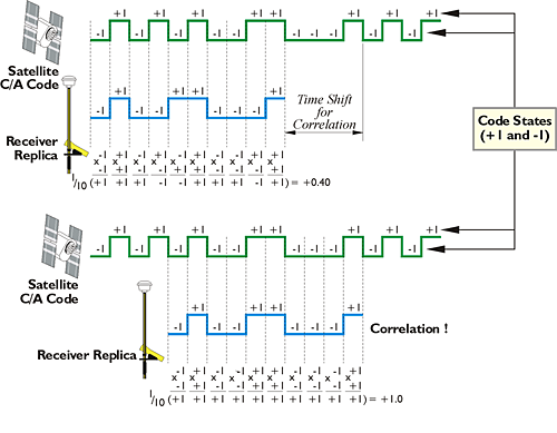
As mentioned earlier, the almanac information from the NAV message of the first satellite a GPS receiver acquires tells it which satellites can be expected to come into view. With this information, the receiver can load up pieces of the C/A codes for each of those satellites. Then the receiver tries to line up the replica C/A codes with the signals it is actually receiving from the satellites. Actually lining up the code from the satellite with the replica in the GPS receiver is called autocorrelation, and depends on the transformation of code chips into code states. The formula used to derive code states (+1 and -1) from code chips (0 and 1) is:
code state = 1-2x
where x is the code chip value. For example, a normal code state is +1, and corresponds to a code chip value of 0. A mirror code state is -1, and corresponds to a code chip value of 1.
The function of these code states can be illustrated by asking three questions: First, if a tracking loop of code states generated in a receiver does not match code states received from the satellite, how does the receiver know? In that case, for example, the sum of the products of each of the receiver’s 10 code states, with each of the code states from the satellite, when divided by 10, does not equal 1. In the example in the illustration, the result is 0.40. Second, what does the receiver do when the code states in the receiver do not match the code states received from the satellite? It shifts the frequency of its search a little bit from the center of the L1 1575.42 MHZ. This is done to accommodate the inevitable Doppler shift of the incoming signal, since the satellite is always either moving toward or away from the receiver. The receiver also shifts its piece of code in time. These iterative small shifts in both time and frequency continue until the receiver code states do in fact match the signal from the satellite. Third, how does the receiver know when a tracking loop of replica code states does match code states from the satellite? In the case illustrated in the image, the sum of the products of each code state of the receiver’s replica 10, with each of the 10 from the satellite, divided by 10, is exactly 1. This is shown in the illustration at "Correlation!" where the receiver’s replica code fits the code from the satellite like a key fits a lock.
The interesting thing is that that time shift for correlation gives the receiver approximately the amount of elapsed time that it took the signal to come from the satellite to the receiver. Obviously, if the receiver knows the elapsed time, and it knows the frequency of the signal, it then knows the distance (the range) between itself and the satellite. This is how the pseudorange works. If this were the whole story, we'd be done, and of course, it isn't the whole story.