Lab 3: Climate Modeling (Introduction)
Lab 3: Climate Modeling
In this activity, we’ll explore some relatively simple aspects of Earth’s climate system, through the use of several STELLA models. STELLA models are simple computer models that are perfect for learning about the dynamics of systems — how systems change over time. The question of how Earth’s climate system changes over time is of huge importance to all of us, and we’ll make progress towards understanding the dynamics of this system through experimentation with these models. In a sense, you could say that we are playing with these models, and watching how they react to changes; these observations will form the basis of a growing understanding of system dynamics that will then help us understand the dynamics of Earth’s real climate system.
What is a STELLA model?
What is a STELLA model?
It is a computer program containing numbers, equations, and rules that together form a description of how we think a system works — it is a kind of simplified mathematical representation of a part of the real world. Systems, in the world of STELLA, are composed of a few basic parts that can be seen in the diagram below:
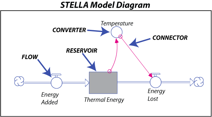
A Reservoir is a model component that stores some quantity — thermal energy in this case.
A Flow adds to or subtracts from a Reservoir — it can be thought of as a pipe with a valve attached to it that controls how much material is added or removed in a given period of time. The cloud symbols at the ends of the flows signify that the material or quantity has a limitless source, or sink.
A Connector is an arrow that establishes a link between different model components — it shows how different parts of the model influence each other. The labeled connector, for instance, tells us that the Energy Lost Flow is dependent on the Temperature of the planet.
A Converter is something that does a conversion or adds information to some other part of the model. In this case, Temperature takes the thermal energy stored in the Reservoir and converts it into temperature.
To construct a STELLA model, you first draw the model components and then link them together. Equations and starting conditions are then added (these are hidden from view in the model) and then the timing is set — telling the computer how long to run the model and how frequently to do the calculations needed to figure out the flow and accumulation of quantities the model is keeping track of. When the system is fully constructed, you can essentially press the ‘on’ button, sit back, and watch what happens.
Introduction to a Simple Planetary Climate Model
Introduction to a Simple Planetary Climate Model
Our first model is slightly more complicated than the diagram shown above because there are quite a few other parameters that determine how much energy is received and emitted and how the temperature of the Earth relates to the amount of thermal energy stored. The complete model is shown below, with three different sectors of the model highlighted in color:
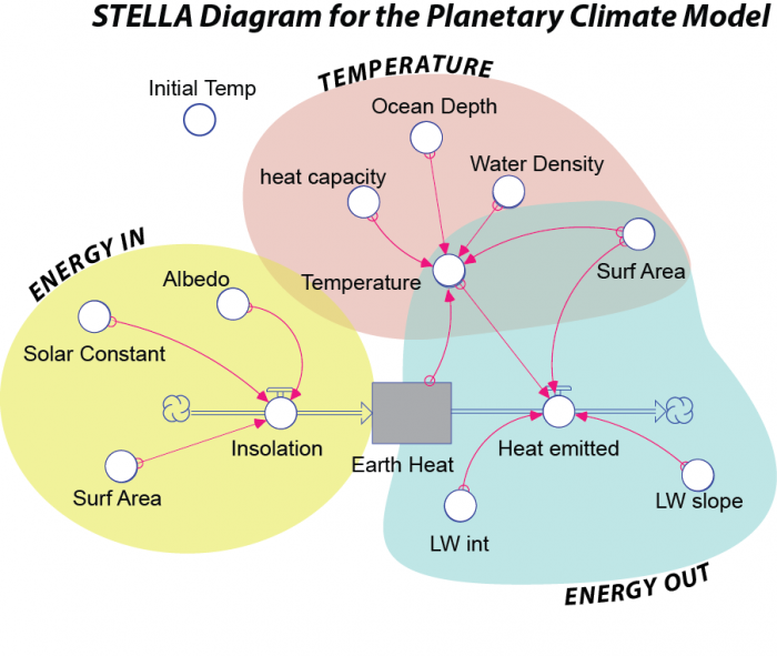
The Energy In sector (yellow above - albedo, solar constant, surf area, and insolation) controls the amount of insolation absorbed by the planet. The Solar Constant converter is a constant, as the name suggests — 1370 Watts/m2. This is then multiplied by the cross-sectional area of the Earth — this is the area that faces the Sun — giving a result in Watts (which you should recall is a measure of energy flow and is equal to Joules per second). This is then multiplied by (1 – albedo) to give the total amount of energy absorbed by our planet. In the form of an equation, this is:
S is the Solar Constant (1370 W/m2), Ax is the cross-sectional area, and a is the albedo (0.3 for Earth as a whole).
The Energy Out sector (blue above - surf area, LW int, LW slope) of the model controls the amount of energy emitted by the Earth in the form of infrared radiation. This is simply described by the Stefan-Boltzmann Law as being the surface area times the emissivity times the Stefan-Boltzmann constant times the temperature raised to the fourth power:
A is the whole surface area of the Earth, e is the emissivity, s is the Stefan-Boltzmann constant, and T is the temperature of the Earth.
The Temperature sector (brown above - water density, ocean depth, heat capacity, temp) of the model establishes the temperature of the Earth’s surface based on the amount of thermal energy stored in the Earth’s surface. In order to figure out the temperature of something given the amount of thermal energy contained in that object, we have to divide that thermal energy by the product of the mass of the object times the heat capacity of the object. Here is how it looks in the form of an equation (with units added):
Here, E is the thermal energy stored in Earth’s surface [Joules], A is the area of the planet [m2], d is the depth of the oceans involved in short-term climate change [m], ρ is the density of sea water [kg/m3] and Cp is the heat capacity of water [Joules/kg°K]. We assume water to be the main material absorbing, storing, and giving off energy in the climate system since most of Earth’s surface is covered by the oceans. The terms in the denominator of the above fraction will all remain constant during the model’s run through time — they are set at the beginning of the model and can be altered from one run to the next. This means that the only reason the temperature changes is because the energy stored changes.
The model has a few other parts to it, including the initial temperature of the Earth, which determines how much thermal energy is stored in the Earth at the beginning of the model run. There are also some converters that divide the energy received and the energy emitted by the surface area of the Earth to give a measure of the intensity of energy flow, of the flux, in terms of Watts/m2, which is a common form for expressing energy flows in climate science.
One unit of time in this model is equal to a year, but the program will actually calculate the energy flows and the temperature every 0.01 years.
Now that you have seen how the model is constructed, let’s explore it by doing some experiments. Here is the link to the model [2].
The First Run
What will happen to the temperature of the Earth if we run the model for 30 years with the following initial conditions:
Initial Temp = 0°C
Albedo = 0.3 (this will not change over time)
Emissivity = 1.0 (this will not change over time)
Ocean Depth = 100 m (this will not change over time)
Solar Constant = 1370 W/m2
These are the values you see when you first launch the model.
Video: Climate Model Introduction (3:22)
Click on the model link. You should see a screen that looks like this, that has a graph here in the middle, that's got different pages you can toggle back and forth between. There's page 1. And then some controls for our model, including the albedo up here, the ocean depth, the emissivity, the initial temperature, and we can change the solar constant here if we want to. So, first, I'm going to run the model and just talk about what we see. So, you click the run button, here, and wait for it to execute. And then, when it's done, it'll display the results of this model run, which is going to go for 30 years here in this case. And here, it's showing us two parameters, one in magenta is the temperature, and it starts off at 0 degrees, because we told it to start at zero. Then, you can see that that temperature drops, and it continues to drop as you move along here and ends up kind of flattening off at a temperature of just about minus 18 degrees Celsius. And that's at about 30 years. Notice that when I put the cursor over one of these curves and then click on the mouse button, it'll tell me the value of that parameter. So, there I can see the temperature at any time the model run. So here, I start off at a temperature of zero, and it cooled very quickly to a temperature of minus eighteen. And that's in part because we have the emissivity here set at one and that means that this model planet has no greenhouse whatsoever. So, this is the presumed temperature of our planet if we had no greenhouse. In this first set of experiments, we're going to have you do a couple of things. One is to change the initial temperature and see to what extent that affects the model's outcome, and then change the albedo up here, and then also change the emissivity. You can change these parameters by doing a couple of things. So, I'm just going to change the initial temperature here to, let's see, 20 degrees, like that. So, I can change it by moving that slider, or I can just click here in this box and type in whatever number I want. So, now I'm going to change it to 10. So, if I do that and then run the model, you can see what happens. It's going to start off at 10 degrees, and then it will evolve after that starting condition. So, here you can see it starts at 10, and it drops off as well. You can restore it to the initial value here by clicking that little “U” and it does undo that change. And then, you can change the emissivity and run it, or change the albedo and run it. After you've made these changes to albedo or emissivity, you want to always click that “U” so you kind of return that value to its starting position. What we're going to do here is to kind of investigate the effects of changing initial temperature, emissivity, and albedo on the performance of this climate model, and we want to look at these things one at a time. Okay, so that's it.
Video: Sample Problem (2:38)
When we ran this initial model, we saw that the temperature of our planet cooled. Here, we see it starting at 10 because that was the last initial temperature that I'd used, and it dropped from 10 to a temperature of about minus 18. Now the question is, why? Why did that happen? Let's consider a couple of things here. We clicked to page two here, we see a couple of other parameters graphed here. One is the energy flux in, so that's just the energy added to our planet in blue. And here's the energy out, the energy flux out, that's the energy leaving the Earth in the form of infrared radiation. And so, look what happens initially. Let's take the energy in to begin with, that starts off with a value of about 240 roughly, 239. Okay, and that doesn't change at all throughout this model run. That has the same value of about 240. And the energy out instead, it starts quite high, 358 watts per meter squared. So, at the beginning of time, the planet is losing a lot more energy than it's gaining here at this blue line. And that continues until eventually, watch that energy flux out, it eventually gets down to be about 240. So, at this point in time, those two have exactly the same value, the energy in and energy out. When the energy in and the energy out have the same value, then our model is in what we call a steady state and the temperature won't change. One thing just to note here is that each of these curves, the red, and the blue, are plotted with their own different scales on the vertical axis. And that's why out in this region here the two curves appear to be offset, but they actually have the same value here, right? So, it's just a little trick in the vertical axis that's misleading us a little bit there. So, the answer to the question of why did the planet cool is simply that, initially given its initial temperature, the energy leaving the planet was much higher than the energy coming into the planet, so the temperature has to drop.
Lab 3: Climate Modeling
Lab 3: Climate Modeling
Instructions
Once you are done answering the questions below, enter your answers into the Module 3 Lab Submission (Practice) to check your answers. If you didn’t do as well as you'd hoped, review the course materials, including the instructional videos, or post questions to the Yammer group to ask for clarification of a particular topic or concept. After that, open the Module 3 Lab Submission (Graded) and complete the graded version of the lab. The graded lab mostly includes questions similar to the practice lab, but has some additional questions.
Download this lab as a Word document: Lab 3: Climate Modeling [4] (Please download required files below.)
Use this Model for Questions 1 - 4. [5] Please Note: The model in the videos below may look slightly different than the model linked here. Both models, however, function the same.
Video: The Simplest Climate Model (Questions 1-3) Part 1 (3:21)
Click on the model link. You should see a screen that looks like this, that has a graph here in the middle, that's got different pages you can toggle back and forth between. There's page 1. And then some controls for our model, including the albedo up here, the ocean depth, the emissivity, the initial temperature, and we can change the solar constant here if we want to. So, first I'm going to run the model and just talk about what we see. So, you click the Run button here and wait for it to execute. And then when it's done, it'll display the results of this model run, which is going to go for 30 years here in this case. And here it's showing us two parameters, one in magenta is the temperature and it starts off at 0 degrees because we told it to start at zero. Then you can see that that temperature drops, and it continues to drop as you move along here, and ends up kind of flattening off at a temperature of just about minus 18 degrees Celsius. And that's at about 30 years. Notice that when I put the cursor over one of these curves and then click on the on the mouse button, it'll tell me the value of that parameters. There I can see the temperature at any time in the model run. So, here I start off at a temperature of zero and it cooled very quickly to a temperature of minus eighteen. And that's in part because we have the emissivity here set at one. And that means that the planet, this model planet, has no greenhouse whatsoever. So this is the presumed temperature of our planet if we had no greenhouse. In this first set of experiments, we're going to have you do a couple of things. One is to change the initial temperature and see to what extent that affects the model's outcome. And then change the albedo up here, and then also change the image emissivity. You can change these parameters by doing a couple of things. So, I'm just going to change the initial temperature here, to let's see 20 degrees, like that. So, I can change it by moving that slider or I can just click here in this box and type in whatever number I want. So, now I'm going to change it to 10. So, if I do that, and then run the model, you can see what happens. It's going to start off at 10 degrees and then it will evolve after that starting condition. So, here you can see it starts at 10 and it drops off as well/ You can restore it to the initial value here by clicking that little "u", it just undoes that change. And then you can change the emissivity and run it or change the albedo and run it. After you've made these changes to albedo or emissivity, you want to always click that "u" so you kind of return that value to its starting position. What we're going to do here is to kind of investigate the effects of changing initial temperature, emissivity, and albedo on the performance of this climate model. We want to look at these things one at a time. Okay. So, that's it.
Video: The Simplest Climate Model (Questions 1-3) Part 2 (2:38)
When we ran this initial model, we saw that the temperature of our planet cooled. Here we see it starting at 10 because that was the last initial temperature that I'd used. And it dropped from 10 to a temperature of minus 18. Now the question is, why? Why did that happen? Let's consider a couple of things here. We clicked to page two here. We see a couple of other parameters graphed here. One is the energy flux in. So that's just the energy added to our planet in blue. And here's the energy out, the energy flux out, that's the energy leaving the earth in the form of infrared radiation. And so look what happens initially. Let's take the energy in to begin with. That starts off with a value of about 240 roughly, 239. Okay. And that doesn't change at all - all throughout this model run. That has the same value of about 240. And the energy out, instead, it starts quite high 358 watts per meter squared. So, at the beginning of time, the planet is losing a lot more energy than it's gaining here at this blue line. And that continues until eventually watch that energy flux out. It eventually gets down to be about 240. So, at this point in time, those two have exactly the same value. The energy in and energy out. When the energy in and the energy out have the same value, then our model is in what we call a steady state and the temperature won't change. One thing, just a note here, is that each of these curves, the red in the blue, are plotted with their own different scales on the vertical axis. And that's why, out in this region here, the two curves appear to be offset but they actually have the same value here, right. So it's just a little trick in the vertical axis that's misleading us a little bit there. So the answer to the question of why did the planet cool, is simply that initially, given its initial temperature, the energy leaving the planet was much higher than the energy coming into the planet. So the temperature has to drop.
Changing Initial Temperature
-
How will changing the initial temperature affect the model? We saw that when we started with an initial temperature (remember that this is the global average temp.) of 0°, the model ended up with a temperature of about -18°C. What will happen if we start with a different initial temperature? Change the initial temperature to 1, then run the model and take note of the ending temperature by placing your cursor over the curve at the right-hand side (where the time is 30 years) and then click and you should see the little box that tells you the position of your cursor. You should round this temperature to the nearest whole number. Select your answer from the following:
A. 10°
B. -8°C
C. -18°C
D. -33°C
Click on the Restore all Devices button when you are done, before going on to the next question.
Changing the Albedo
-
What will happen to our climate model if we change the albedo? Recall that a low albedo represents a dark-colored planet that absorbs lots of solar energy, while a higher albedo (it can only go up to 1.0) represents a light-colored planet that reflects lots of solar energy. Change the albedo to 0.5, then run the model and find the ending temperature, and select your answer from the following:
A. about -38(plus or minus 1)
B. about 2 (plus or minus 1)
C. about -1 (plus or minus 1)
D. about -16 (plus or minus 1)
Click on the Restore all Devices button when you are done, before going on to the next question.
Changing the Emissivity
-
Next, we will see what happens when we change the emissivity. Recall that if the emissivity is 1.0, the planet has no greenhouse effect and as the emissivity gets smaller, it represents a stronger greenhouse effect — so, how will this change our climate model? Change the emissivity to 0.3, then run the model and find the ending temperature, and select your answer from the following:
A. about -18 (plus or minus 1)
B. about 47 (plus or minus 1)
C. about 16 (plus or minus 1)
D. about 71 (plus or minus 1)
Click on the Restore all Devices button when you are done, before going on to the next question.
Changing the Solar Constant
Video: The Simplest Climate Model (Question 4) (3:24)
Click here for a transcript of The Simplest Climate Model video.For problem number four, we're gonna see what happens to the climate model in response to a brief change in the solar constant. We’re gonna increase the solar constant for a little bit and see how the model reacts. But before doing that, we're going to try to set the model up, to begin with, in such a way that it represents something like our earth. So, we're going to change the emissivity first to .61, that's an emissivity value that kind of represents the strength of our greenhouse. We're going to change the initial temperature of our planet to 15 and we'll leave the other things the same. Then we're going to go to the solar constant here and click on that. And right here in the middle of this graph, I'm going to position the cursor right here and click one little tick mark up. There, so I've made a graph now of the solar constant so that it's steady at 1370, then it bumps up to 1372 here for a little bit, and then it drops back down like that to 1370 for the rest of the time. You hit okay, and now we're ready to run the model to see what happens. So, it's evaluating it and we're about to see the results here. So, we see in magenta now the temperature of our climate model is staying constant at 15, up until the point where the solar constant starts to increase. And then, as it increases, the planetary temperature increases to 15.05, it peaks there. And notice that that peak occurs at 16.6 years, 16.7 years, something like. That's about 1.7 years after the peak in the solar constant value. So, that's what we call a lag time, a difference in time between the peak of some kind of forcing (like the solar constant) and the response, which is the planetary temperature. So, it peaks at about 1.7, 1.8 years later. And then it drops back down. It doesn't quite get back down to 15 after we have restored the solar constant to 1370, because the system takes a while to sort of settle down again and that's a function of the kind of thermal mass of the climate system, which is related to the ocean temperature. And so, what we're going to do in this in this question, is to change the ocean depth from its default value of 100 to different values, by simply typing in a different value here. So, there's 200, and then running the model and comparing the response of the model to this kind of control version here that we're looking at in this little video. So you might want to, in fact, you should, take note of the maximum temperature rise of the model, following this spike in the solar constant, and the timing of that as well.
Credit: Dutton [3]The solar constant is not really constant for any length of time. For instance, it was only 70% as bright early in Earth’s history, and it undergoes smaller, more rapid fluctuations (and much smaller) in association with the 11-year sunspot cycle. Let’s see how the temperature of the planet reacts to changes in the solar constant. First, we need to run a “control” version of our model, as is shown in the video above. Set the model up with the following parameters:
Initial Temp = 15°C
Albedo = 0.3
Emissivity = 0.6147 (enter the value manually in the box)
Ocean Depth = 100 m
Solar Constant — alter graph as shown in the video. Note the lines in the Solar Constant graph do not line up exactly with numbers. To get the exact number (1372) click on the Solar Constant Plot, then on Graph and enter the value at X=15 Y-1372.
Record the peak temperature (should be 15.04 deg C) and the time lag (should be 1.7 years).
-
What we are going to look at now is how the ocean depth affects the way the model responds to this spike in the solar constant. In our control, the ocean depth is 100 m — this means that only the upper 100 m of the oceans are involved in exchanging heat with the atmosphere on a timescale of a few decades. If the oceans were mixing faster, this depth would be greater, and if they were mixing more slowly, the depth would be less. Change the ocean depth to 50 m. Then run the model and note the peak value of the temperature and estimate the lag time, for comparison with the control version. Select your answer from the following:
A. Peak temp > control; lag time > control
B. Peak temp < control; lag time > control
C. Peak temp > control; lag time < control
D. Peak temp < control; lag time < control
Adding a Feedback
Use this Model for Question 5. [6] Please Note: The model in the videos below may look slightly different than the model linked here. Both models, however, function the same.
Now, we’re ready to try something more challenging and more realistic. In the real world, the surface temperature has a big impact on the albedo — when it gets very cold, snow and ice will form and increase the albedo. So, there is a feedback in the system — a temperature change will cause an albedo change, which will cause a temperature change, and so forth. To explore this feedback, we need to work with an altered version of the model [7], where we have defined the relationship between albedo and temperature as follows:
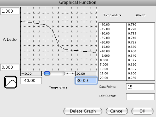 Relationship between albedo and temperature in the revised modelCredit: David Bice © Penn State University is licensed under CC BY-NC-SA 4.0 [1]
This graph implies that there is a kind of threshold temperature of about -10 to -15°C, at which point the whole planet becomes frozen. The suggestion is that even with a very cold global temperature of 0 °C, the equatorial region might be relatively ice-free and would thus have a low albedo, but as the temperature gets colder, even the tropics become covered by snow and ice. Once that happens, the planetary albedo changes only slightly. Likewise, at higher temperatures, the albedo decreases only slightly since there is so little snow and ice to remove.
This important to understand what this model includes — a link between planetary temperature and planetary albedo. As the temperature changes, so the albedo changes, and as the albedo changes, so the insolation changes, and as the insolation changes, so the temperature changes — this is a feedback mechanism. Feedback mechanisms are very important components of many systems, and our climate system is full of them.
Video: Simple Planetary Climate Model (Question 5) (4:20)
Click here for the Simple Planetary Climate Model (Question 5) video.For problem number five, we have a slightly different model of the climate system that's got a few new features to it. We see the initial temperature and albedo and ocean depth from before. The solar multiplier here is just something that, if it's one, it's not going to change the solar input at all. If I make that greater, like 2 or 1.5 or 3, or something, that's going to increase, it's going to multiply solar constant by 1.3 in this case. I'm going to do that here. It also has something called a CO2 multiplier and it does the same thing to the CO2 concentration. So, here it is set at 1 initially. I could make that 2 and then in that case instead of having 380 parts per million CO2, we'd have 760. So, we would double it. And if I made this be 0.5 then we would cut our CO2 concentration in half, and in doing that, we're changing the greenhouse effect of the climate model. We could change the history of atmospheric CO2 using this graph here, but we're not going to work with that in number five. It also has a couple of switches down here, one for a solar cycle and one for the albedo switch. And this albedo switch is the most important thing for this problem. When it's in this position, it's off. And then, we have just a constant albedo that's assigned up here in this box. But if we turn that thing on by going “click”, like that, it's suddenly now is going to make the albedo be a function of temperature, and that creates a feedback mechanism that does some interesting things. You'll kind of explore that in this problem. Let me just show you a few things here. So, if we restore everything to the way it was when you first opened the model and you just run it. You see that in page 1 of this graph pad, everything is just constant all the way across here. CO2, solar input, and temperature are staying the same. I'm going to switch to page 3 of this and this shows the temperature for the first run here. Now, if I switch the albedo switch on, I'm activating that feedback mechanism. But if I run it, it doesn't change anything at all. Okay, now watch this. I'm going to turn that back off. I'm going to decrease the CO2 multiplier. I'm going to make it be point something very small, point one, let’s say. Let's change that to point one, and now I'm going to run the model and see what happens. So, it gets quite a bit colder because we've taken a lot of CO2 out of that atmosphere here. It gets down to 8.3 at the end of eighty years. Now, if I turn the albedo switch on, see what happens now. Now, the temperature really drops. It drops to -5.6. So, the difference between -5.6 and this 8.3, that's the impact of the feedback mechanism. It has an effect, a cooling effect, from 8.3 to -5.6, so something more than 13 degrees of a negative shift in temperature for that feedback mechanism. So, in this problem, you're going to be assigned a CO2 multiplier value and you'll type that in here. It'll be something like 0.25 or 0.5 or 2 or 4 or something along those lines. You enter that number in there. Let's say you've got 4, and then you run the model with the albedo switch off and then you run it again with the albedo switch on, and you look at the temperature difference between those two runs of the model to get a sense of how big the albedo feedback effect is in our climate system.
Credit: Dutton [3]By definition, feedback mechanisms are triggered by a change in a system — if it is in steady state, the feedbacks may not do much. In the above graph, you may notice that at a temperature of 15°C (our steady state temperature), the albedo is 0.3, which is the albedo of our steady state model. So, if we run the model with an initial temperature of 15 °C, and an unchanging solar constant of 1370, our system will be in a steady state and we will not see the consequences of this feedback. But, if we impose a change on the system, things will happen.
The change we will impose involves the greenhouse effect. The model includes something called the CO2 Multiplier. When this has a value of 1, it gives us a CO2 concentration of 380 ppm, which is the default value that gives us a temperature of 15°C. If we change it to 2, we then have 760 ppm and a stronger greenhouse, which leads to warming. If we change it to 0.5, we then have 190 ppm and a weaker greenhouse, thus cooling.
You will be given a value for the CO2 Multiplier; enter that into the model and run it with the Albedo Switch in the off position (see the video) and note the ending temperature. Then turn the Albedo Switch on, which activates the feedback mechanism, and run the model again, noting the ending temperature. The difference between these two temperatures is what you need for your answer. For example, if you set the CO2 Multiplier to 3 and run the model with the Albedo Switch turned off, you see an ending temperature of 18.17°C, and then with the switch turned on, the ending temperature is 24.86°C, so the temperature difference due to the albedo feedback is +6.69°C — this is the answer you would select.
Set the CO2 Multiplier to 6.0
-
What is the temperature difference due to the albedo feedback? Choose the answer that most closely matches your result. Be sure to study page 3 of the graph pad to get your results.
A. about -5°C
B. about +11°C
C. about +18°C
D. about -20°C
Causes of Climate Change
Use this Model for Questions 6-7. [8] Please Note: The model in the videos below may look slightly different than the model linked here. Both models, however, function the same.
Things that can cause the climate to change are sometimes called climate forcings. It is generally agreed upon that on relatively short time scales like the last 1000 years, there are 4 main forcings — solar variability, volcanic eruptions (whose erupted particles and gases block sunlight), aerosols (tiny particles suspended in the air) from pollution, and greenhouse gases (CO2 is the main one). Solar variability and volcanic eruptions are obviously natural climate forcings, while aerosols and greenhouse gases are anthropogenic, meaning they are related to human activities. The history of these forcings is shown in the figure below.
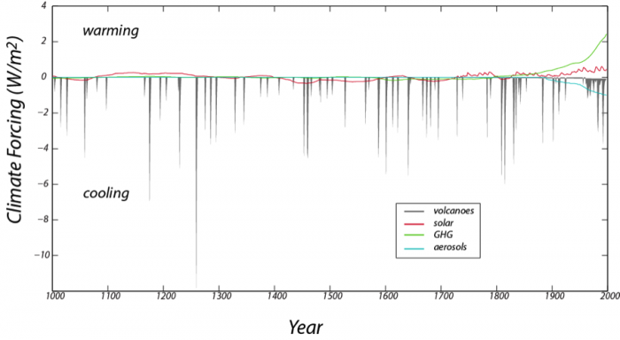 The reconstructed record of important climate forcings over the past 1000 years (data from Crowley, 2000). Positive values lead to warming, while negative values lead to cooling. Note that although volcanoes have very strong cooling effects, these effects are very short-lived.Credit: David Bice © Penn State University is licensed under CC BY-NC-SA 4.0 [1]
Volcanoes, by spewing ash and sulfate gases into the atmosphere block sunlight and thus have a cooling effect. This history is based on the human records of eruptions in recent times and ash deposits preserved in ice cores (which we can date because they have annual layers — we count backward from the present) and sediment cores for older times. Note that although the volcanoes have a strong cooling effect, the history consists of very brief events. The solar variability comes from actual measurements in recent times and further back in time, on the abundance of an isotope of Beryllium, whose production in the atmosphere is a function of solar intensity — this isotope falls to the ground and is preserved in ice cores. The greenhouse gas forcing record is based on actual measurements in recent times and ice core records further in the past (the ice contains tiny bubbles that trap samples of the atmosphere from the time the snow fell). The aerosol record is based entirely on historical observations and is 0 earlier in times before we began to burn wood and coal on a large scale.
In this experiment, we will add the history of these forcings over the last 1000 years and see how our climate system responds, comparing the model temperature with the best estimates for what the temperature actually was over that time period. Solar variability, volcanic eruptions, and aerosols all change the Ein or Insolation part of the model, while the greenhouse gas forcing change the Eout part of the model. We can turn the forcings on and off by flicking some switches, and thus get a clear sense of what each of them does and which of them is the most important at various points in time.
We can compare the model temperature history with the reconstructed (also referred to in the model as “observed”) temperature history for this time period, which comes from a combination of thermometer measurements in recent times and temperature proxy data for the earlier part of the history (these are data from tree rings, corals, stalactites, and ice cores, all of which provide an indirect measure of temperature). This observed temperature record, shown in graph #1 on the model, is often referred to as the “hockey stick” because it resembles (to some) a hockey stick with the upward-pointing blade on the right side of the graph.
First, open the model [9]with the forcings built-in, and study the Model Diagram to get a sense of how the forcings are applied to the model. If you run the model with all of the switches in the off position, you will see our familiar steady state model temperature of 15°C over the whole length of time. The model time goes from the year 1000 to 1998 because the forcings are from a paper published in 2000.
Graph #1 plots the model temperature and the observed temperature in °C, graph #2 plots the 4 forcings in terms of W/m2, graph #5 plots the cumulative temperature difference between the model and the observed temperature (it takes the absolute value of the temperature difference at each time step and then adds them up — the lower this number at the end of time, the closer the match between the model and the observed temperatures), and graph #6 shows the same thing, but it begins keeping track of these differences in 1850, so it focuses on the more recent part of the history. Graph #1 gives you a visual comparison of the model and the observed temperatures, while graphs #5 and 6 give you a more quantitative sense of how the model compares with reality.
Video: A Simple Climate Model with 1000 years of Forcings (Questions 6-7) (3:33)
Click here for a transcript of the Simple Climate Model with 1000 years of Forcings (Questions 6-7).The model that you're going to use for problems six and seven is this one here. It's the same climate model that we've worked at before, in essence, but here we're running it for a much longer time, from the year 1000 up until 1998. And over that time, we're applying to the model, the best estimates of four different climate forcings, things that can change the climate. One is greenhouse gas concentrations, another is aerosols, these are fine particulates, essentially pollution in the atmosphere. Then there are volcanic forcings, so whenever there is an eruption, all the particles thrown up into the atmosphere tend to block sunlight and cause cooling. And then there's a solar variability, that's another forcing, and that changes over the course of time as the Sun gets brighter or dimmer. So, each of these forcings has a switch associated with it. You can turn them. They’re in the on position now. You can turn them off here, and we'll just run the model really quickly here, and you'll see two things on this graph. One is in red, the model temperature, so our climate model temperature, about 15 degrees steady through time. And then, in blue, is the observed temperature. This is the reconstructed temperature over this time period based on all sorts of studies of different climate proxies. And so, the idea is that if we have a relatively good climate model and we apply these four principal forcings to it, we should be able to kind of closely match this observed temperature curve here in blue. So, we can turn these things on and see what they do. There's the greenhouse gas concentration, here's the aerosol concentration combined with greenhouse gases. And I'm going to combine the volcanic forcing, and finally, the solar forcing. So, we see all four kinds of principal climate forcings added in here. One variable here is the ocean depth, the depth of the ocean water that's involved in relatively short-term climate change. Watch what happens if I increase that. I’ll just increase it to four hundred and something. I'll run it again and watch what happens to these abrupt little cooling spikes that are associated with volcanic eruptions. You see they get diminished greatly if the ocean depth is greater, and that's just because these volcanic eruptions are such short-lived forcings, that if the ocean that's involved in climate is very deep, it doesn't change much, it doesn't have time to change much, because these volcanic events are so short. So, that really dampens the cooling effect there and you get a much closer match to the curve here. So, in these questions, you'll be asked to try out various combinations of these forcings and evaluate the match between the model temperature and the observed temperature here, and there are two questions to answer with respect to this model.
Credit: Dutton [3] -
Before running the model set the ocean depth to 50 m. Run the model 4 times with each of the forcing switches turned on separately (i.e., only one forcing switch turned on for each model run) and evaluate which of the forcings does the best job of matching the shape of the observed temperature curve from 1800 to 1998. Which one provides the best match?
A. GHG
B. Aerosols
C. Volcanoes
D. Solar
-
Before running the model, set the ocean depth to 150 m. Run the model 3 times — once with only the natural forcing switches turned, once with only the anthropogenic forcings turned on, and once with all of them turned on. Which combination does the best job of matching the shape of the observed temperature curve from 1800 to 1998?
A. natural forcings
B. anthropogenic forcings
C. all forcings
D. natural and anthropogenic forcings are about the same.