Effects of Pumping Wells

Effects of Pumping Wells 

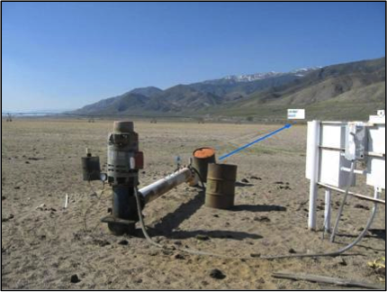
Groundwater is accessed by either pumping from wells drilled into the aquifer (Figure 33), or by developing natural springs where the potentiometric surface intersects the land surface (Big Spring in Bellefonte, PA is one example of a relatively large spring that is used for municipal supply). Although springs are relatively inexpensive to develop, they are not always present, nor are the flow rates always sufficient to support demand. As a result, most groundwater extraction occurs by pumping wells, or in many cases “fields” of wells concentrated in a small area.

Figure 33. Example of groundwater extraction well in the Garden of Cambremer, France

Source: Philippe Alès (Own work) CC-BY-SA-3.0, via Wikimedia Commons (top)

 

Figure 34. Example of an irrigation well in Walker Lake, NV

Source: USGS Nevada Water Science Center, photo by Lindsay R. Burt (bottom)

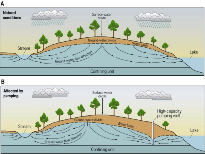
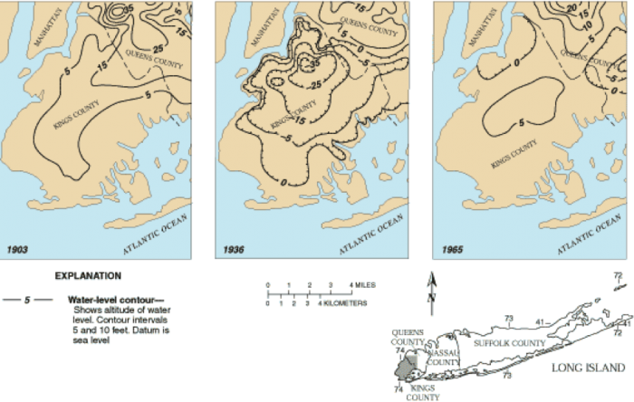
Cones of Depression: Pumping at a well, or at a wellfield, pulls water toward the well from all directions – in other words, it induces radial flow (around the radius of the well). In doing so, pumping causes a reduction in hydraulic head, known as drawdown. This drawdown generates a cone- or funnel-shaped depression called a cone of depression (Figure 35). The reduction in hydraulic head drives groundwater flow to the well (in the down-gradient direction), as shown in the example from Long Island in Figure 36.

Figure 35. Schematic cross-section showing the effects of pumping and generation of a cone of depression in an unconfined aquifer between a lake and a stream. Pumping and the ensuing cone of depression reverse the hydraulic gradient from pre-development (A) and induce flow from the stream into the groundwater system and to the well(B)

Click for more information

Two similar images. Image A is under natural conditions while image B shows the effect of pumping. Both diagrams show the same piece of land with a lake on the right, a stream on the left, a ground-water divide at a water table, with a surface-water divide right above it, and a confining unit beneath the groundwater flow. Diagram A shows an equal groundwater flow direction to the stream and the lake split at the ground-water divide. Diagram B has a high capacity pumping well close to the lake causing a cone of depression. Water flows from the ground-water divide to the stream as before but also to the well. Water is also pumped from the lake to the well instead of flowing out to the lake.

Source: USGS: Groundwater in the Great Lakes Basin: the case of southeastern Wisconsin

Figure 36. Potentiometric surface for southwestern Long Island, New York, ca. 1903 (pre-development), 1936 (near the peak in pumpage for combined municipal and industrial uses), and 1965, well after the municipal supply was switched to the upstate supply system described in Liquid Assets, and after reduction in withdrawals for industrial use.

Source: USGS

Both the width and the depth of the cone of depression scale with the rate of pumping, the aquifer permeability, and storativity, and the duration of pumping. In general, larger cones of depression result from larger pumping rates, higher permeability or lower storativity, and longer elapsed time.  If cones of depression from two separate pumping wells grow large enough to overlap, it is known as well interference. When well interference occurs, the respective drawdowns are added together. The result is that drawdown is accelerated when multiple cones of depression interact. This is generally not desirable, and is one important consideration in the design, permitting, and operation of wells.

Not only does the cone of depression draw water to the well, but if the pumping rate is large enough or pumping is sustained for a long time, it can reverse the natural hydraulic gradient hundreds of meters to several tens of km away from the well(s). In some cases, this may result in interception of groundwater that would normally feed a stream or river as baseflow, and even in the interception of streamflow itself by inducing infiltration in the stream bed or banks (Figure 35B). In other cases, large cones of depression (up to a few miles wide!) associated with industrial or municipal well fields may reverse regional topographically-driven hydraulic gradients and lead to problems like saltwater intrusion (Figure 35B).