Supply Curve

Everything in the realm of costs that we have talked about - returns to a factor, fixed and variable costs, economic profits - help define the supply curve.

What is the supply curve? Like the demand curve, it is a Functional Relationship. It is a relationship between the amount of money a firm is willing to accept in exchange for a certain amount of some good. It is not a constant. Because of the notion of declining marginal returns, we can assume that as we produce more of a good, the marginal cost of that good increases. This means that supply curves slope upwards. According to the law of supply, there is a positive relationship between the price of a good or service and the amount of it that suppliers are willing to produce. Meaning that if price increase, producers will supply more.

In reality, most marginal costs curves are U-shaped - they start very high at low volumes of production, they decrease as more of a good is made (economies of scale), and then as diminishing returns kicks in, the curve starts to rise again. There are some industries in which the marginal cost - that is, the cost of serving one more customer - continually slope downwards, like the utilities.This is a special case we will talk about later.

So, the supply curve is a relationship that tells us the minimum amount that a firm is willing to accept for selling a unit of a good. What is this minimum amount? Well, if you are a firm and you need to make one more unit of a good, then the cost to you of that good is the marginal cost of that good. To make the good, you need to recover, at a minimum, your marginal cost. Therefore, the supply curve IS the marginal cost curve.

First, we need to find the $Q_1$ and $Q_2$. We can do that using supply function:

We can find the total cost and marginal cost for Q=1 to 10 as:

Table 3.7 Marginal Cost Chart

Q	TC	MC
1	8
2	13	5
3	20	7
4	29	9
5	40	11
6	53	13
7	68	15
8	85	17
9	104	19
10	125	21

Individual Supply Curve

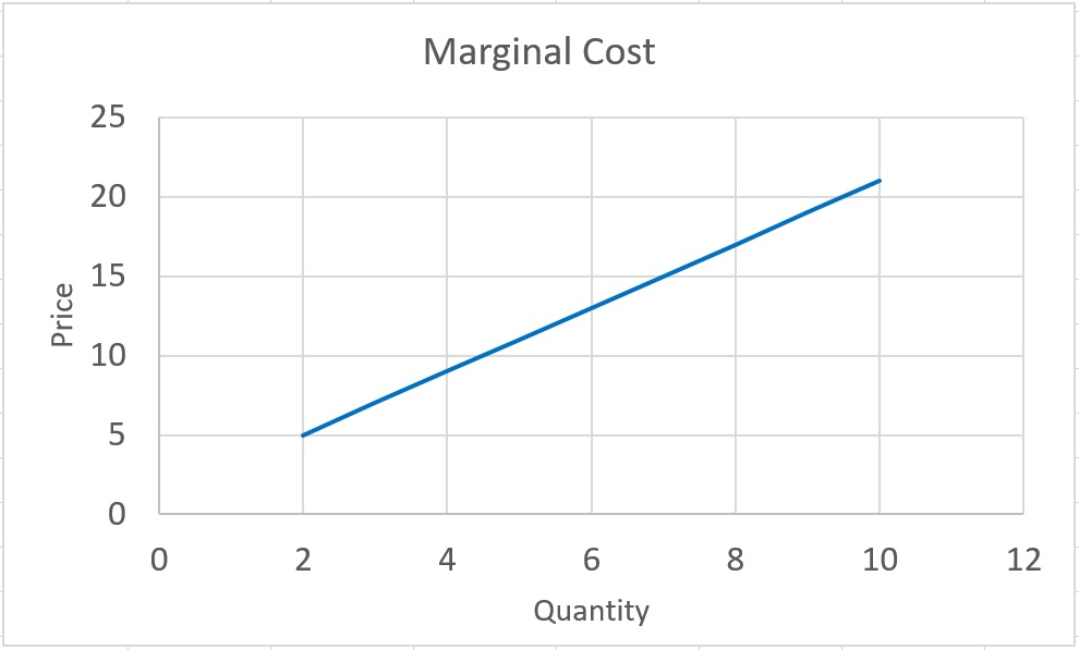
Following graph displays the marginal cost (price) on the y-axes versus quantity on the x-axes. This curve is the supply curve (function) for the supplier. As we can see, it is an upward line. So, in order to find the supply curve (function), we need to extract the marginal cost from the total cost function. This graph tells us if price is $15, this producer is willing to produce 7 unites of the good. Or, for example, the minimum amount of money that this producer is willing to exchange for producing 4 units, is $9.

Note that market supply curve is the summation of all individual producer supply curves.

Producer surplus

Similar to the concept of consumer surplus that we learnt in Lesson 2, we can define the producer surplus. Let’s start with an example. Assume you own a pizza shop and you are willing to make and sell pizza if price is at least $1.5 per slice. However, the market price is $2 per slice and you can sell each slice at the market price and receive $2. The difference between $2 and $1.5 is your net gain from exchanging the pizza with money. This gain is called your producer surplus. Producer surplus is the difference between minimum price you are willing to make and sell, and the amount you actually receive from selling the pizza. Please note that this gain is different from profit.

Let’s assume market production for a good equals $P=4+2Q$

So, if the market price is $20, market will supply 8 unites of the good $\left(20=4+2Q;Q=8\right)$ . And we know that $P=4+2Q$ is the market supply function, which is the summation of all individual supply functions.

Let’s say the first producer is willing to supply the first unit of the good to the market at the price of 6 dollars (you can plug Q=1 to the supply function). However, the market price is $20. So, his individual gain (individual producer surplus) from producing and selling, will be $14 $\left(20-6\text{=14}\right)$ . And if we do this for all other unites of the good, we can find the individual producer surplus for other suppliers in the market. And if we add them all together, we can calculate the total producer surplus in the market.

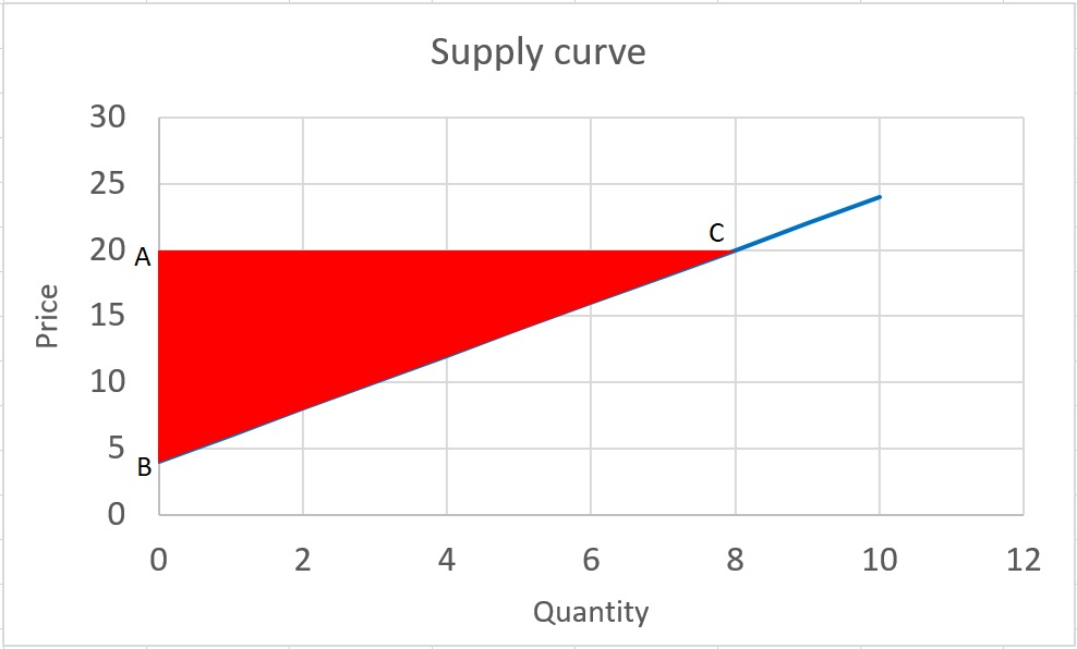
You might have already noticed that for finding the total market producer surplus, we just need to find the area of the triangle, which is bounded to supply curve, market price (horizontal line), and the y axis.

For calculating the area, we need to find the length of two sides $\left(A-B\text{and}B-C\right)$ :

A represents the market price and the coordinate will be (0, $20)
B is the supply curve intercept and the coordinate will be (0, $4)
C is the market supply at price = $20, and you can find the coordinate simply by plugging P=20 into the supply function $\left(20=4+2Q;\text{ Q=8}\right)$ . And the coordinate of C will be (8, $20)

Now that we have the coordinates, we should be able to calculate the area of triangle as:

$PS=\left(20-4\right)*\left(8-0\right)/2=64$

So, producer surplus at market price of P=$20 will be 64.

Note that, in general, when we are talking about the producer surplus, we refer to the market producer surplus, which is the summation of all individual supplier producer surplus. So, to calculate the producer surplus, we need to find the area above the supply curve and below the price. This area represents the total producer surplus in the market.

Price elasticity of supply

Similar to the method that we used to calculate the price elasticity of demand, we can define and calculate price elasticity of supply as:

“Percentage change in quantity supply, divided by percentage change in the price causing the supply response.”

$\eta =\%\Delta Q/\%\Delta =\left[\left(Q_2-Q_1\right)/Q_1\right]/\left[\left(P_2-P_1\right)/P_1\right]$

The Greek letter eta $\eta$ is used to denote elasticity.

Price elasticity of supply reflects the sensitivity of suppliers to the price changes. Note that, since supply curve is upward, the price elasticity of supply is a positive number.

Example: Following the previous example find the elasticity of supply when price increase from $20 to $24.

First, we need to find the $Q_1$ and $Q_2$. We can do that using supply function:

$\begin{array}{l}{P}_1=\$20\\ P_1=4+2Q_1\\ 20=4+2Q_1\\ 24-4=2Q_1\\ Q_1=8\end{array}$ $\begin{array}{l}{P}_2=\$24\\ 24=4+2Q_2\\ 24-4=2Q_2\\ Q_2=10\end{array}$ $\eta =\left[\left(Q_2-Q_1\right)/Q_1\right]/\left[\left(P_2-P_1\right)/P_1\right]=\left[\left(10-8\right)/8\right]/\left[\left(24-20\right)/20\right]=1.25$

We can also calculate the midpoint elasticity as:

$\eta =\left[\left(Q2-Q1\right)/\left(Q1+Q2\right)\right]/\left[\left(P2-\text{P}1\right)/\left(P1+\text{P}2\right)\right]=\left[\left(10-8\right)/\left(10+8\right)\right]/\left[\left(24-20\right)/\left(24+20\right)\right]=1.22$