As explained before, in sensitivity analysis, we aim to discover the magnitude of change in one variable (here, output variables) with respect to change in other variables (here, input parameters). Then, we can rank the variables based on their sensitivity. It helps the decision-maker to understand the parameters that have the biggest impact on the project.
The following example introduces a single variable sensitivity analysis. Please note that here we assume variables are independent and have no effect on each other. For example, it is assumed that the magnitude of initial investment doesn’t affect the operating costs.
Example 6-1:
For a project, the most expected case includes an initial investment of 150,000 dollars at the present time, an annual income of 40,000 for five years (starting from the first year), and a salvage value of 80,000. Evaluate the sensitivity of the project ROR to 20% and 40% increase and decrease in initial investment, annual income, project life, and salvage value.
Before-tax cash flow of this investment can be shown as:
|
-$150,000
|
$40,000
|
$40,000 | $40,000 | $40,000 | $40,000 |
$80,000
|
|
|
||||||
|
0
|
1
|
2
|
3
|
4 |
5
|
|
The most expected ROR based on the most expected initial investment, annual income, and salvage value can be calculated as:
The most expected ROR will be 20.5%.
A) Sensitivity Analysis of initial investment
| Initial investment | Change in prediction | ROR | Percentage change in 20.5% ROR prediction |
|---|---|---|---|
| 90,000 | -40% | 43.5% | 112.7% |
| 120,000 | -20% | 29.6% | 44.8% |
| 150,000 | 0 | 20.5% | 0% |
| 180,000 | 20% | 13.8% | -32.6% |
| 210,000 | 40% | 8.6% | -57.8% |
As you can see, changes in ROR with respect to changes in initial investment are considerably high. In general, parameters that are close to time zero have a higher impact on the ROR of the project.
B) Sensitivity Analysis of project life
| Project life | Change in prediction | ROR | Percentage change in 20.5% ROR Prediction |
|---|---|---|---|
| 3 | -40% | 12.9% | -36.6% |
| 4 | -20% | 17.7% | -13.5% |
| 5 | 0 | 20.5% | 0% |
| 6 | 20% | 22.2% | 8.7% |
| 7 | 40% | 23.4% | 14.5% |
Note that changes in the project ROR become smaller as the project life gets longer.
C) Sensitivity Analysis of annual income
| Annual income | Change in prediction | ROR | Percentage change in 20.5% ROR prediction |
|---|---|---|---|
| 24,000 | -40% | 8.1% | -60.6% |
| 32,000 | -20% | 14.3% | -30.0% |
| 40,000 | 0 | 20.5% | 0% |
| 48,000 | 20% | 26.5% | 29.5% |
| 56,000 | 40% | 32.4% | 58.5% |
Changes in annual income also have a significant effect on ROR because these changes start happening close to present time.
D) Sensitivity Analysis of salvage value
| salvage value | Change in prediction | ROR | Percentage change in 20.5% ROR prediction |
|---|---|---|---|
| 48,000 | -40% | 17.0% | -17.0% |
| 64,000 | -20% | 18.8% | -8.2% |
| 80,000 | 0 | 20.5% | 0% |
| 96,000 | 20% | 22.0% | 17.7% |
| 112,000 | 40% | 23.5% | 14.8% |
We can conclude that salvage value has the least effect on the ROR of the project because salvage value is the last amount in the future and its present value is relatively small compared to other amounts.
The following figure displays a tornado chart that is a very useful method to graphically summarize the results of sensitivity analysis. The right and left hand side of each bar indicate the maximum and the minimum ROR that each parameter generates when changed from -40% to +40%.
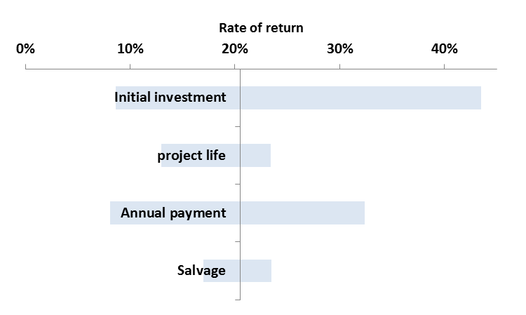
| Type | Rate of Return Range |
|---|---|
| Initial investment | 8.6% - 43.5% |
| Project life | 13% - 23.4% |
| Annual payment | 8.1% - 32.4% |
| Salvage | 17% - 23.5% |
Please watch the following video (18:02): Sensitivity Analysis.
PRESENTER:
In this video, I will work on an example and explain the sensitivity analysis method. I will describe how we can use this method for project evaluation. Let's work on a simple example.
In this example, we will run single variable sensitivity analysis. We also assume all the input variables are independent and have no effect on each other. For instance, we assume the magnitude of initial investment has no effect on operating costs.
This investing project requires $150,000 of investment at the present time and it yields the annual income of $40,000 for five years from year one to year five and the salvage value of $80,000 in the end of the year five. And we want to evaluate the sensitivity of the project rate of return to 20% and 40%, change increase and decrease in initial investment, annual income, project life, and salvage.
First we calculate the rate of return on this cash flow for this project. The present value of costs equals present value of income plus present value of salvage. And we will find that we will solve this equation for i using the IRR function in Excel or any other spreadsheet. And we calculate the rate of return on this cash flow as 20.5%.
First, sensitivity analysis of initial investment. So in the first step, we want to see what would be the rate of return for this project if we decrease the initial investment by 40%. It means we have to multiply this under $50,000 by 1 minus 40%. So it is going to be $90,000. So if the initial investment of the project decreases by 40%, then we will have the initial investment of $90,000 at present time.
And we calculate the rate of return for this new situation. Present value of cost equals present value of income plus present value of salvage. And we calculate the rate of return as 43.5%.
Now effect of 20% decrease in the initial investment. So the initial investment, if it is decreased by 20%, is going to be 1 minus 20%, multiply $150,000. And we calculate the rate of return for the new situation, for the case that we have 20% less initial investment. And the rate of return is going to be 29.6%.
The third case is when we calculate the rate of return for a 20% increase in initial investment. So initial investment is going to be 1 plus 20%, multiply $150,000, which is going to be $180,000 of investment. And the rate of return can be calculated as present value of cost equals present value of income plus present value of salvage. And the rate of return will be 13.8% if the initial investment is increased by 20%.
And the fourth case is when our initial investment is increased by 40%, which is going to be 1 plus 40%, multiply $150,000, which comes to $210,000. And the rate of return is calculated as 8.6% if the initial investment is increased by 40%.
And this table summarizes the result for sensitivity analysis on initial investment. So the third row is the base case when there is no change in our initial investment. The rate of return, as we calculated, was 20.5%. If the initial investment is decreased by 40%, then the rate of return for this project is going to be 43.5%, which will be 112.7% higher than the base case that we had.
Initial investment is decreased by 20%, then the rate of return is going to be 29.6%, which, comparing to the base case, the rate of return is going to be 44.8% higher than the base case. If the initial investment is increased by 20%, then rate of return is going to be 13.8, which is going to be around 33% lower than the base case. And the last case, if the initial investment is increased by 40%, then the rate of return for the project is going to drop to 8.6%, which is 58% lower than the base case that we had.
Now let's do the sensitivity analysis for the project lifetime. The project lifetime is initially five years. So the 40% decrease in project lifetime is going to be 1 minus 40, multiply 5, which is going to be three years. So the project with the initial investment of-- we hold every other thing constant. So the project with initial investment of $150,000 and annual income of $40,000 for three years and the salvage value of $80,000. We calculate the rate of return, which is going to be 12.9%.
And then effects of a 20% decrease in project lifetime. So if the project lifetime is decreased by 20%, you're going to have four years, 1 minus 20% multiply by five, which comes to four. And a calculation of rate of return for the new cash flow, we're going to have four years of income of $40,000. And rate of return is going to be 17.7%
Of 20% increase in project life, which is going to be 1 plus 20%, multiply 5, which is going to be 6 year. One year increase in project lifetime, in this case, we are going to have a rate of return of 22.2%. And if the project lifetime is increased by 40%, meaning that we add two more years to the lifetime of the project, one plus 0.4, multiply 5, equals to 7. We have two more years of project lifetime. And the rate of return can be calculated as 23.4.
And we summarize the sensitivity analysis of project life result in this table. So the third row is the base case. Project life is initially five years. And the rate of return is 20.5%.
If the project life is decreased by 40%, we are going to have three years of project life and the rate of return is going to be 12.9%. If the project life is decreased by 20%, then the rate of return is going to be 17.7%, which is 13.5% less than the base case. If the project life is increased by 20%, then we can see it is going to have positive impact on the rate of return, which is 8.7% higher than the base case, higher than 20.5%. And if the project lifetime is increased by 40%, the project life is going to be seven years and the rate of return is going to be 23.4, which is 14.5% higher than the base case, which was 20.5%.
And now sensitivity analysis for annual income. The initial value for annual income was $40,000. 40% decrease means 1 minus 40%, multiply $40,000, and we're going to have the annual income of $24,000. We calculate the rate of return for such projects. So every other thing is the same. We just decrease the annual income by 40%. So the rate of return is going to be 8.1%. [AUDIO OUT].
The effect of 20% decrease in annual income will be 1 minus 20%, multiply $40,000, which is going to be $32,000. We're going to have $32,000 if the annual income is decreased by 20%. And the rate of return for such project is going to be 14.3%.
We will repeat these calculations for 20% increase in annual income. If annual income from the base case is increased by 20%, we are going to have 1 plus 20%, multiply $40,000, which gives $48,000 of annual income per year for five years. And the rate of return is going to be 26.5%.
We'll repeat the calculations for a 40% increase in annual income, which is going to be 1 plus 40%, multiply $40,000, which comes to $56,000 annual income. So if our annual income is increased by 40% from the base case, we are going to have $46,000 per year. And the rate of return in this new case will be 32.4%.
So, again, this table summarizes the sensitivity analysis of annual income. The base case is when we have $40,000 of income per year. The rate of return is going to be 20.5%. If the annual income is decreased by 40%, we are going to have $24,000 per year and the rate of return is going to be 8.1%, which is going to be 60.6% lower than the base case, lower than the base case of 20.5%.
If the annual income is decreased by 20%, we are going to have $32,000 per year and the rate of return is going to be 14.3%, which is almost 30% less than the base case. If annual income is increased by 20%, we are going to have $48,000 dollars per year and the rate of return is going to be increased to 26.5%, which is 29.5% percent higher than the base case. And in the end, if annual income is increased by 40%, we will have the annual income of $56,000. And rate of return is going to be 32.4%, which is 58.5% percent higher than the base case.
And the last part, we are on the sensitivity analysis for the salvage value. The initial value for salvage is $80,000. 40% decrease in salvage value can be calculated as 1 minus 40%, multiply $80,000, which comes to $48,000. And the rate of return for this change, $40,000 of salvage, which is here, is going to be 17%.
We'll repeat the calculations for 20% decrease in salvage. 1 minus 20%, multiply $80,000, which is going to be $64,000 of salvage. And the rate of return, 18.8%. Percent.
We will calculate this for 20% increase in salvage. 1 plus 20%, multiply $80,000 equals $96,000. And the rate of return can be calculated as 22%. And the last one, 40% increase in salvage value, which will be 1 plus 40%, multiply $80,000, equals $112,000 of salvage value. And rate of return will be 23.5.
This table summarizes the sensitivity analysis of salvage value. The third row is the base case. There is no change in any input variable and the rate of return is 20.5%.
The first row is the case that we have 40% decrease in salvage value. In this case, the rate of return is going to be 17%, which is 17% lower than the base case, which was 20.5%. If the salvage value is decreased by 20%, then rate of return is going to be 18.8%, which is 8.2% lower than the base case.
If the salvage value is increased by 20%, the rate of return is going to be 22%, which is 7% higher than the base case. Last row, which shows the 40% increase in salvage. And the rate of return in this case is going to be 23.5%, which is almost 15% higher than the base case of 20.5%.
This table summarizes the sensitivity analysis result for these four input variables. So the second row is the base case where nothing has changed. So rate of return is 20.5%.
The first row shows if the input is decreased by 40%. So if the initial investment is decreased by 40%, then rate of return is going to be 43.5%. If the project lifetime is decreased by 40%, we can see it has a negative effect on the rate of return. The rate of return is going to decrease to 12.9% and so on.
The last row shows the result if the input variable is increased by 40%. So if the initial investment is increased by 40%, rate of return is going to be 8.6%. If the project life is increased by 40%, rate of return is going to be 23.4 and so on.
We can also summarize these results in a graph called tornado graph. And we can see here this vertical line shows the base case where nothing has changed. The rate of return is 20.5%. This bar shows what would be the change in the rate of return of the project if initial investment changes from 40% positive to 40% negative, 40% increase to 40% decrease.
Credit: Farid Tayari
If you are interested, the following video (10:48) explains how to draw a tornado chart in Microsoft Excel (please watch from 6:10 to 9:00).
CHARLIE NUTTELMAN: This screencast is going to go over a sensitivity analysis, and we're going to generate a tornado plot. A sensitivity analysis is basically a study into how sensitive is the process, so the process outputs, to the inputs. So just as an example here, we have a process, and it's got a bunch of inputs, and it may have one or more outputs.
An example might be a reactor where the inputs would be things like the temperature, the pressure, maybe the size, the flow rate, concentration of different things, and so on. And the outputs might be conversion. Just a simple example. And we want to determine how sensitive the outputs of the process are to the inputs.
The specific example I'm going to be working with has to do with net present value. We've made a screencast on this already, and you don't necessarily have to understand this net present value example. It has to do with engineering economics and determining the net present value of a venture 15 years from the current time. We have different inputs to the process. The inputs would be things like the cost of land, the cost of royalties per year, the total depreciable capital-- that's how much you have to invest in major equipment-- working capital, startup costs.
We have sales, which is S. Other inputs include tax, because tax rates might change. And cost of sales, here we have 6 million. And we have an interest rate, or the cost of capital. So again, you don't necessarily have to understand exactly what I've done in this spreadsheet to understand sensitivity analysis. The important thing is that we have a process and we have multiple inputs that go into determining what the output is. And for this process, the output is down here.
This tells us that the net present value of a venture based upon our base case, or our baseline or nominal values of these different variables up here, the net present value that is about 58 million. We're going to now do a sensitivity analysis. We're going to see what happens when we change different values here for the cost of land, maybe the annual sales, and annual costs, and so on. So what happens, maybe, if we subtract 20% from the nominal values and increase 20%?
So you'll notice here, I have 58.78 million down here. And if I change something like cost of sales, let's just say to eight, instead of being 58.78, it's a lot less. It's 50.30. So you can see that this process, the output which is net present value, depends upon the input variable. So I'm going to put that back to six. And maybe I change land to instead of 5 million, it's negative 4 million but that didn't change it a whole lot. It was 58.78, and now it's 59.78. So I'm going to put that back to minus five.
We're going to do a data table to look at these different input variables and what effect they have on the output. So we're going to do a sensitivity analysis first on the working capital. The nominal value, or the baseline value, for working capital is negative 20 million. That's how much we're going to request for working capital. And we want to ask ourselves how sensitive is the net present value after 15 years? How sensitive is that to the working capital? So if we have 80%, that'd be minus 16 instead of minus 20, as opposed to 120%, which is negative 24.
So all I've done here is multiply our baseline value of negative 20, which is up here in our spreadsheet. I multiplied that by 80%, all the way up to 120%.
We're going to make a data table here. When you make a data table, we have a column of different inputs that we're going to do kind of a case study on, the cell one up and one over from our values. This is a pointer formula, so I'm going to do equals. We're pointing to our net present value. That's the result. And then what I can do is highlight all of this, our column of cells, plus one row above. And I'm going to go into Data, What If Analysis, Data Table. And this is a column data table. And each of these working capital values is going to be placed into cell B4 up here.
And so I'm going to press OK, and it's going to do sort of a case study on that. I forgot to mention one thing. If I just did a multiplication of cell C33 here, which is negative 20, times the percentage and created a vector here, I actually have to copy and paste so that's not a formula. Because if this is a formula and we put that into the data table, it doesn't quite work right. So we have to copy and paste the values so they're just numbers instead of formulas in this column before we do the data table.
So this is telling us if the working capital is negative 16, the net present value is about 62.5 million. And if we increase it by 20%, we see that the net present value is about 55 million. So I can go through all of these different values. And the green here represents the baseline values. So we have working capital, which I showed you. I did this for startup costs, sales, the interest rate or cost of capital, the land costs, total depreciable capital, capital, and cost of sales.
And what I've done for all of these, I've taken the minus 20, which is our 80% of nominal cost, and our 120% of that particular variable and I've made a summary table here. What we're going to do now is create something known as a tornado plot. To create the tornado plot, I'm going to highlight one of these rows. I go up here to Insert, Chart, and we're making a clustered chart, a clustered bar chart. And right now, it's not looking anything like a tornado plot, but bear with me here.
I'm going to format this a little. I'm going to go over here and add in axis titles. I'm going to add in a legend. I'm going to go back up here, and I'm going to copy, so I'm selecting this, Control + C. That's the 120%. And I'm going to click in the area, do Control paste. Now, again, this isn't looking really like a tornado plot, but we have some work to do. We need to change this. I'm going to do Format Axis, and it's going to cross axis values. Vertical axis crosses axis value at 58.78. That was our nominal value.
So if I go back up here, 58.78 is the net present value when we have 100% of all those values. That was our base case. Now this is sort of looking like a tornado diagram. And I'm going to click on one of these series, Format Data Series. We're going to do 100% overlap, sort of eclipsing. And I'm going to make this a little bigger. I'm going to decrease the gap width, maybe something around 60%.
We can further modify this. So I'm going to right-click on this axis, Format Axis. Let's change the number to be zero decimals. I'm also going to click on the category over here, and we will format that. So I'd right-click on this, format that axis. I'm going to change the labels so they are low. What that does is it brings those labels to the left side.
And another thing I'm going to do is change those labels. So I'm going to do Select Data. Instead of these one, two, through eight, I'm going to edit that, and that's going to be named our categories up here. So I can do that. Click OK. And it has added those different categories.
And the last thing we need to do is to change our legend. So I'm going to bring the legend inside here so I can expand this a tiny bit. And I can right-click in here and do Select Data. And I'm going to change this to minus 20%. I'm editing the series, and this will be plus 20%. And we're pretty much done. So that is a tornado diagram.
And what this tornado plot shows us is that if we change, for example, sales, if that goes down by 20% of our baseline, then that has a huge effect on the net present value. Same thing with if we increase sales by 20%. That has a very big effect on net present value. Some other things that don't have as big of effect, you see that C_land doesn't have a big effect. If your land costs vary tremendously, that's not going to have a huge effect on net present value at all. But if your sales are off of what you're anticipating, then this can have a huge effect on the net present value.
So that's varying from around 20 million to 100 million, which is a huge difference there. And your boss might say, if you gave him this sensitivity plot, your boss might say, well, we need to put a lot more effort into making sure we have a really good estimate on sales. Because if sales are 20% lower than what we're expecting, then the profitability of this venture's way lower than if our sales are 20% higher than what we're expecting.
This sort of tells you what are the main players in your output, and the output, in this case, is net present value. And if you really wanted to, you could organize this. You can put the big bars up at the top and the small ones at the bottom, and it sort of looks like a tornado, so that's what the tornado plot gets its name. OK, thanks for watching this screencast.