The expected value is defined as the difference between expected profits and expected costs. Expected profit is the probability of receiving a certain profit times the profit, and the expected cost is the probability that a certain cost will be incurred times the cost.
Example 6-2:
A wheel of fortune in a gambling casino has 54 different slots in which the wheel pointer can stop. Four of the 54 slots contain the number 9. For a 1 dollar bet on hitting a 9, if he or she succeeds, the gambler wins 10 dollars plus the return of the 1 dollar bet. What is the expected value of this gambling game? What is the meaning of the expected value result?
- 0.185 dollars indicates that if the gambler plays this game over and over again, the average gain for the gambler per bet equals - 0.185 dollars, which means the gambler will lose 0.185 dollars per bet. Note that for a satisfactory investment, a positive expected value is a necessary, but not sufficient, condition.
Example 6-3:
Assume drilling a well costs 400,000 dollars. There are three probable outcomes:
a) 70% probability that the drilled well is a dry hole
b) 25% probability that the drilled well is a producer well with such rate that can be sold immediately at 2,500,000 dollars
c) 5% probability that the drilled well is a producer well with such rate that can be sold immediately at 4,000,000 dollars
Calculate the project's expected value.
Note that +425,000 dollars is a statistical term; it means the average of +425,000 dollars will be achieved in the long-term for drilling over and over again in a repeated investment of this type.
Expected NPV and Expected ROR Analysis
Example 6-4:
Assume a research project that has the initial investment cost of 100,000 dollars. There are two possible outcomes:
a) 30 % success: that leads to an annual profit of 60,000 dollars for five years (starting from year 1) with a salvage value of zero
b) 70 % failure: that leads to annual profit and salvage value of zero
Considering a minimum 12% discount rate, compare the expected NPV, and explain if this investment is satisfactory.
| 30 % success: | -$100,000 | $60,000 | $60,000 | $60,000 | $60,000 | $60,000 |
| 70 % failure: | -$100,000 | 0 | 0 | 0 | 0 | |
|
|
||||||
| 0 | 1 | 2 | 3 | 4 | 5 | |
Since considering risk in calculations results in negative expected Net Present Value (ENPV), it can be concluded that this investment is expected to be economically unsatisfactory. Note that risk-free NPV (assuming 100% success probability) shows good and economically satisfactory results.
Example 6-5:
Calculate the expected Rate of Return for the above example.
Expected ROR is the “i” that makes Expected NPV equal 0.
Expected Present worth income @ "i" – Present Worth Cost @"i" = 0
By trial and error, Expected ROR = - 3.4%
Note that risk free ROR shows a satisfactory result.
Risk-free ROR = 52.8%, which is much higher than the minimum ROR.
Another way to calculate the expected ROR, which is similar to the previous method, is to calculate expected cash flow and then find the ROR for that.
Expected cash flow can be determined by multiplying each scenario’s cash flow by its probability and then make summation over each year:
| Year 1 | Year 2 | Year 3 | Year 4 | Year 5 | |
|---|---|---|---|---|---|
| Expected cash flow |
Then:
| Year 1 | Year 2 | Year 3 | Year 4 | Year 5 | |
|---|---|---|---|---|---|
| Expected cash flow | -$100,000 | $18,000 | $18,000 | $18,000 | $$18,000 |
By trial and error, Expected ROR = - 3.4%
Please watch the following video (14:01): Expected Value Analysis, Part I.
PRESENTER: In this video, I will explain the second method to incorporate risk and uncertainty in project evaluations. This method is called expected value analysis, and the expected value is the difference between expected profits and expected costs. Expected profit is the probability of receiving a profit multiplied by the profit, by the payoff, and the expected cost is the probability that certain costs will be incurred multiplied by that cost.
Let's assume a wheel of fortune that has 24 slots, and three of these slots have a red color. So you randomly turn this wheel of a slot, and if you get a red color, you will win $5. And if you get any color other than red, you will lose $1. So let's see what would be the expected value of this game and what is the meaning of the expected value results?
So the probability of success is 3/24, and the probability of failure is going to be 21 divided by 24. So the expected value equals the expected value of profit minus the expected value of cost. The expected value of this game is minus $0.25. So it means that if we play this game over and over again, the average gain per bet, the average gain per game, is going to be $0.25. So if we play this game over and over again, we will lose $0.25 per game.
Let's work on this example. Assume a drilling well that costs $400,000, and there are three possible outcomes. We have a 70% probability that we get a dry hole, which means there will be no outcome and we just have the cost of $400,000 at the present time. There is a 25% probability of success that we get a producer well, which can be immediately sold at a price of $2.5 million. And we have a 5% probability that we drill a well that is a producer and can be sold immediately at $4 million.
Let's calculate the project's expected value. So this is the expected value of failure, 70% multiplied by we have just $400,000 of cost. There is no income revenue or profit, in this case. And we have two cases of success. We have 25% of success that we get a producer well and we can sell it at $2.5 million, but we still have the $400,000 of costs. And also, we have another success case with a probability of 5% that is going to yield $4 million of immediate income, and we have $400,000 of drilling cost.
And the summation is going to be $425,000, the expected value of this project. So in each case, we multiply the probability of that event by the outcome of that event. So this is the outcome. This is the failure case. This is the outcome of the failure, and this is the probability. Here, this is one of the success cases. This is a 25% probability of success. And in case of success, we are going to have $2.5 million, but still, we have to pay the drilling cost and so on.
Please note that the $425,000 of expected value for this project is a statistical term, and it means that the average of $425,000 will be achieved in the long term. If we do this drilling, if we play this game, if we drill this field over and over again, holding the probabilities and costs and incomes constant, this is the expected value that we are going to achieve after doing the drilling again, over and over again.
Another example. Let's assume an investment project requires the initial investment cost of $100,000, and there are two possible outcomes. There is 30% of success that leads to an annual profit of $60,000 for five years, equal payments of $60,000 for five years. The salvage value is going to be zero. And the 70% failure that we receive nothing. There is no annual profit, and salvage would be zero.
Let's calculate the expected NPV for this project, assuming the minimum discount rate of 12%. So we draw these two cases in the timeline. There is 30% of success that we have $100,000 of cost at the present time. And in this case of success, we are going to have a $60,000 annual income of $60,000 per year from year one to year five. In case of failure, we still need to pay the initial costs for this project, but we will earn nothing in the future years.
So in this case, we need to calculate the NPV of each case, multiply that by the probability, and then make a summation over all the possible cases. So here we have a 30% probability of success. This is the NPV of success. This shows the NPV of success. We have $100,000 of cost at the present time, and we have five equal payments of $60,000 from year one to year five.
Probability of failure. Multiply the failure case, NPV of failure, which is going to be just the $100,000 of cost at the present time, and the expected NPV for this project, which is a negative value.
So if we consider risk in this project, meaning that we are assuming a 30% probability for success and 70% probability for failure, we are going to have expected-- We are going to have negative expected NPV, which means that this project is not a good project for investment. Note that the risk-free NPV, meaning that the probability of success is 100%, is going to be a positive number, which means this project is economically satisfactory.
Now, let's calculate the expected rate of return for this example. Again, the example is the same. We have a project that requires $100,000 of investment at the present time. There is 30% of success that yields $60,000 of income for five years from year one to year five, and there is a 70% of failure that we will earn nothing, the annual profit, and the salvage value will be zero.
So the expected rate of return is the rate that makes the expected NPV equal zero. So the equation for expected rate of return is expected present value of incoming equals expected present value of cost. So in case of success, we are going to have $60,000 for five years. And the probability is the present value of the $60,000, and this is when we multiply that with the probability of success, it gives us the expected present value of income.
And on the right-hand side, we are going to have the expected value of cost, which is going to be $100,000 if we have in case of success, multiplied by the probability of success. And also, plus $100,000 in case of failure, multiplied by the probability of failure. And you can see because this cost is shared between these two cases, so it stays unchanged. Because the decimation of this probability equals, these two probabilities equal one. So the expected present value of income equals the expected present value of cost and solving this equation for i, we'll get the rate of return of minus 3.4%.
There is another way to calculate the expected rate of return for this project, which we can calculate the expected rate of return from the expected cash flow. How do we calculate the expected cash flow for each year, for each column? We calculate the expected money that will happen in that year. For example, this year, we have $100,000 of investment with a probability of 30% plus $100,000 of investment at a probability of 70% failure and for the year one, we are going to have $60,000 of income. But the probability of this income is going to be 30%. So $60,000 multiplied by 30%.
And we have zero income with a probability of 70%, which I didn't write it here because it equals zero. And same for the other years. And we calculate the summation. So in each year, we write the expected cash flow. We write the expected money that is going to happen in that year. For year one, we are going to have the $100,000 of investment. Again, because this investment is shared, is common for both failure and success, it stays unchanged. But for the other years, because we have income only for the success scenario, we multiply the $60,000 of income by 30%. And we are going to have $18,000 for the year one to year five.
So we can calculate the rate of return, the same as what we used to do for cash flow. It might be easier to just write the rate of return equation for this cash flow. We have $100,000 of costs, and we have $18,000 of income from year one to year five. The present value of cost equals the present value of income. And we solve this equation using Excel or any other spreadsheet.
Example 6-6:
Calculate Expected NPV for a minimum ROR 20% to evaluate the economic potential of buying and drilling an oil lease with the following estimated cost, revenues, and success probabilities.
The lease would cost 100,000 dollars at time zero and it is considered 100% certain that a well would be drilled to the point of completion one year later for a cost of 500,000 dollars. There is a 60% probability that well logs look good enough to complete the well at year 1 for a 400,000 dollar competition cost. If the well logs are unsatisfactory, an abandonment cost of 40,000 dollars will be incurred at year 1. If the well is completed, it is estimated there will be a 50% probability of generating production that will give 450,000 dollars per year net income for years 2 through 10 and a 35% probability of generating 300,000 dollars per year net income for years 2 through 10, with a 15% probability of the well completion being unsuccessful, due to water or unforeseen completion difficulties, giving a year 2 salvage value of 250,000 dollars for producing equipment.
The above decision-making process can be displayed in the following figure. These types of graphs are called decision trees and are very useful for risk involved decisions. Each circle indicates a chance or probability node, which is the point at which situations deviate from one another. (Costs are shown in thousands of dollars.)
Note: Times 1 and +1 are the same points in time and both indicate the end of year 1. The main body (of the tree) starts from the first node on the left with a time zero lease cost of 100,000 dollars that is common between all four situations. The next node, moving to the right, is the node that includes a common drilling cost of 500,000 dollars. At this node, an unsatisfactory and abandonment situation with a cost of 40,000 dollars in the first year (situation D) deviates from other situations (a branch for situation D deviates from the tree main body). The next node on the right (third node) is the node where situations A, B, and C (three separate branches) get separated from each other. At the beginning of each branch is the probability of that situation, and at the end of it, amounts due to that situation (including cost, income, and salvage value) are displayed.
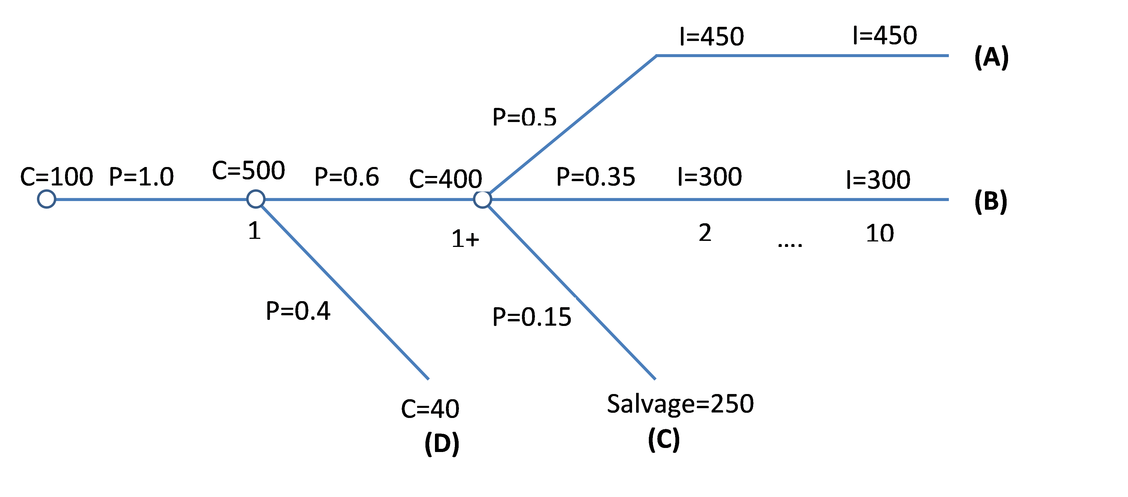
So, there are four stations:
Situation A: Successful development that yields the income of 450 dollars per year
Situation B: Successful development that yields the income of 300 dollars per year
Situation C: Failure that yields a salvage value of 250 dollars at the end of year two
Situation D: Failure that yields abandonment cost of 40 dollars at the end of year one
Probability of situation A can be calculated as
Probability of situation B can be calculated as
Probability of situation C can be calculated as
Probability of situation D can be calculated as
| Probability | |||||||
| A) |
0.3
|
C=$100 | C=$500+$400 | I=$450 | I=$450 | ... | I=$450 |
| B) |
0.21
|
C=$100 | C=$500+$400 | I=$300 | I=$300 | ... | I=$300 |
| C) |
0.09
|
C=$100 | C=$500+$400 | Salvage=$250 | 0 | ... | 0 |
| D) | 0.4 | C=$100 | C=$500+$40 | 0 | 0 | ... | 0 |
|
|
|||||||
| 0 | 1 | 2 | 3 | ... | 10 | ||
Note that the summation of all properties should equal 1.
Project ENPV is the summation of ENPV for all situations. So, first, we need to calculate ENPV for each situation:
And it can be summarized in Table 6-1 as:
| Probability | Year 1 | Year 2 | Year 3 | Year 4 | ... | Year 5 | ENPV | |
|---|---|---|---|---|---|---|---|---|
| A | 0.3 | -$100 | -$900 | $450 | $450 | ... | $450 | $198.5 |
| B | 0.21 | -$100 | -$900 | $300 | $300 | ... | $300 | $33.1 |
| C | 0.09 | -$100 | -$900 | $250 | 0 | ... | 0 | -$60.9 |
| D | 0.4 | -$100 | -$540 | 0 | 0 | ... | 0 | -$220 |
Project ENPV is slightly less than zero compared to the total project cost of 1 million dollars, therefore, slightly unsatisfactory or breakeven economics are indicated.
Please watch the following video (13:32): Expected Value Analysis, Part 2.
PRESENTER: Let's work on a more complicated example. Let's assume a drilling project.
The lease costs would be $100,000 at time 0. That will be paid for all the cases. Then we will have the $500,000 of drilling costs at year 1. Again, this cost is paid for all the cases.
After we paid these $500,000 of drilling costs, we get to the completion point. At this point, there is 60% probability that well logs are good enough to complete the well, which is going to cost $400,000. And there is a 40% failure that they don't look good enough. And we need to close the wells and pay the abandonment cost and so on.
So in case of the 60% probability, let's call it a success case, we will pay $400,000 more in the same year 1 for completion costs. In this case, we will face three cases. One case with a probability of 50%, we will have a producer well, which is going to produce $450,000 per year of income from year 2 to year 10.
And the second case, we are going to have a 35% probability of a well that is going to generate $300,000 per year from year 2 to year 10. And we will have a 15% probability of that the well completion being unsuccessful. And we will have a salvage value of $250,000 for producing equipment in year 2.
So we can summarize the information here. There will be $100,000 of lease costs for all the cases at the present time. And there will be $500,000 of drilling cost at year 1 for all the cases. And then we'll have a 60% probability of getting to the completion. In this case, we pay another $400,000 in year 1. And if I weight 40% probability if we don't complete the well, we need to pay and order $40,000 of costs at year 1.
So in the case of 60%, we will face three new cases. 50% probability that generates $450,000 from year 2 to year 10. And case two, 35% probability of generating $300,000 from year 2 to year 10. And a 15% probability that we don't end up doing anything, any money, any producing well. And we have just a salvage value of $250,000 in year 2.
So the decision tree is a very helpful graph that can help us separate the possible cases here. So I will explain this in this graph. So we start from the left-hand side, the initial investment for the lease at the present time. We write the cost or income here. And in front of that, we write the probability.
So this probability is 100% because it is the same for all the cases. At year 1, we spend $500,000 for drilling, and then, in this case, we are going to have two branches being deviated from the main branch. One is 60%, let's call it a success here, a 60% probability of success and a 40% probability of failure. In case of failure, we are going to pay $40,000 of closing costs, abandonment costs.
In case of success, 60%, we will face another three cases. In case of success, we will pay another $400,000 of completion costs. This 1 plus is to show that this is the same year as this year. These are happening in the same year. But because these cases deviate from the main branch, we draw another branch for these, to separate these from the main branch.
So 60% of success, we pay $400,000 of completion cost. And we will have three new cases in the after. So there is a 50% chance, there is a 50% probability that we will earn $450,000 from year 2 to year 10. So years are here.
So every value under the same column has the same year dimension. We have 35% of getting $300,000 from year 2 to year 10. And we have a 15% probability that we get only $250,000 of salvage at year 2.
So as we can see here, we have four main cases here. Case A, case B, case C, and case D. So the first step to approach this problem and calculate the expected NPV is to calculate the probability of each case. So in order to calculate the probabilities of each case, we go back to the decision tree.
We start from the right-hand side for each case. For example, for case A. So I start from the right-hand side. For example, case A, I start moving from the right-hand side toward the left.
I have a 50% probability here. And go to the main branch. I have a 60% probability here. And I have a 100% probability here. So I will multiply.
I start moving from the right-hand side along each branch to the left, and I multiply the probabilities that I see on the way. So here, I have a 50%, and 60% probability, and a 100%. So I will multiply 50% multiply 60% probability and 100% which has no effect. So the probability of A is 50% multiplied 60%.
B, the probability of case B is 35%, multiply 60%. And multiply this 100%, which has no effect. Case C, probability of 15%, multiply 60%. And case D, the probability of 40% multiply 1, which is going to be 40%. So I calculate the probabilities for case A, case B, case C, and case D.
In the second step, I draw the timeline and I separate the cases from each other. In the first row I write the probabilities. Case A, there is a $100,000 lease cost at the present time. Drilling costs at year 1, plus $400,000 of completion costs.
You remember this was in case the well logs look good. So this $400,000 happens in the same year. And case A is going to generate $450,000 from year 2 to year 10.
Case B, $100,000 of lease costs, plus $500,000 of drilling, plus $400,000 of completion costs. This was happening in year 1. The lease cost is at year 0. And the income from year 2 to year 10.
Case 3. Case 3, the lease cost, the drilling costs, and the completion costs are $400,000 in year 1. And I'm going to have just the salvage of $250,000 in year 2. And the income for other years is going to be 0.
So in case D, which I call it failure case. I pay the lease cost at the present time. I pay the drilling cost in year 1. But the well logs are not looking good enough to pay the completion costs. So I will just close the well and pay the abandonment cost of $40,000.
So now that I have this table calculating the expected NPV. For each case, I calculate the NPV and I multiply that by the probability. And I make a summation over all that.
So here, you can see this is the equation for case A to calculate the NPV. This is the lease cost at the present time. It doesn't need to be discounted.
This is the summation of $500,000 of drilling cost, plus $400,000 of the completion costs. And the $450,000 of income from year 2 to year 10, which they are 9 equal series of income payments. And I need to discount this for one year because they start from year 2.
And the NPV for case B, case C, and case D. Please note that the salvage is happening at year 2 for case C, so I need to discuss that for two years. And I write the NPV for each case in the last column. I multiplied probability by the NPV for each case. And I wrote that too in this column.
And the summation of all these values here is going to give me the expected NPV for this project. And as you can see here, it is going to be about minus $50,000. And the conclusion would be because the expected NPV is slightly negative, is slightly less than 0. We can conclude that this project is not very economically satisfactory.
Credit: Farid Tayari
Italicized sections are from Stermole, F.J., Stermole, J.M. (2014) Economic Evaluation and Investment Decision Methods, 14 edition. Lakewood, Colorado: Investment Evaluations Co.