Lessons
Lesson 1: Introduction to Remote Sensing
Lesson 1 Introduction
A brief history of remote sensing as a governmental activity, a commercial industry, and an academic field provides the student with a perspective on the development of the technology and emergence of remote sensing applications. Accounts of remote sensing history generally begin in the 1800s, following the development of photography. Many of the early advancements of remote sensing can be tied to military applications, which continue to drive most of remote sensing technology development even today. However, after WWII, the use of remote sensing in science and infrastructure extended its reach into many areas of academia and civilian life. The recent revolution of geospatial technology and applications, linked to the explosion of computing and internet access, brings remote sensing technology and applications into the everyday lives of most people on the planet. One could argue that there are very few aspects of life that are not touched in some way by this powerful and enabling way of viewing, understanding, and managing our world.
This lesson will also introduce the basic scientific principles of light and its interaction with matter that makes remote sensing possible. This foundation will be drawn upon throughout the course to explain how remotely sensed imagery is acquired, processed, and analyzed. Many new terms will be introduced and carefully defined, in this lesson and throughout the rest of the course. While some of these terms may seem familiar, many are often misused in casual communication. It is a responsibility of the remote sensing or geospatial professional to inform and guide those with whom he/she comes in contact, through correct and precise use of these terms.
Throughout this course, you will be guided to many external resources that you can use to complement the course material and continue to refer to after completing the course.
Lesson Objectives
At the end of this lesson, you will be able to:
- describe key milestones in the historical development of remote sensing;
- discuss fundamental principles of electromagnetic radiation that are the basis for remote sensing;
- summarize the role of remote sensing as a fundamental element of GIS analysis.
Questions?
If you have any questions now or at any point during this week, please feel free to post them to the Lesson 1 Questions and Comments Discussion Forum in Canvas.
History of Remote Sensing and Photogrammetry
In Chapter 1 of the textbook, Introduction to Remote Sensing, Jim Campbell provides a narrative of the evolution of remote sensing and photogrammetry over the past two centuries. Some of this history is brought to life in a series of short videos, produced by ASPRS [1].
Watch this video about Aerial Survey Pioneers (1:47).
Video: Aerial Survey Pioneers (High Def) (1:47)
JIM LIVING: Back in 1923, Talbert Abrams bought an airplane, and he was barnstorming. And he found out that people would pay him more to take pictures of their farms and buildings than they would to go for a ride in the airplane. It was people like him that started this whole industry.
MO WEINBERG: Mapmakers, topographers, from the four different sections of the country would bring about a revolution in map making.
MORRIS THOMPSON: They were in an airplane, open cockpit, no shelter. After you get the aerial photos, what do you do with them?
MARILYN O'CUILINN: They saw the possibilities of mapping from the air.
WILLIAM A. RADLINKSKI: Most of the farmers didn't know how many acres they had, so we would determine which acreage was tillable. And that was called mapping.
ALFRED O. QUINN: I tried to get mathematics with Professor Earl Church. But the only course that I could get with him was once known as photogrammetry.
DON LAUER: I had a plan to play for the Army All-Star Basketball team. But Bob had a vision. He convinced me to go to graduate school, profound experience.
MORRIS THOMPSON: I only know of one person around here who would still remember so much detail. And he wasn't there when it began, and I was.
Watch this video about geospatial intelligence in WWII (1:58).
Video: Geospatial Intelligence in WWII (High Def) (1:58)
MARILYN O'CUILINN: Photogrammetry started with the military.
On Screen Text: “The nation with the best photo reconnaissance will win the next war.” General Werner von Fritsch, Chief of the German General Staff, 1938
[Dramatic music]
On Screen Text: Case Study: Chattanooga, TN -1939 TVA-USGS team during WWII
MORRIS THOMPSON: We had a combined TVA-USGS force. When the war started in Europe, we got to wondering about who is next.
On Screen Text: a shift in focus…..
MO WEINBERG: Map making was turned over to the Army map service, so that we would map for them.
MORRIS THOMPSON: And where do you suppose we started? China? Japan? Where? Upstate New York.
On Screen Text: defending our coasts
VIRGINIA LONG: They thought the Germans would invade the United States by way of the Saint Lawrence Waterway.
MORRIS THOMPSON: But that's just the beginning.
On Screen Text: mapping enemy territory
On Screen Text: Army Air Corps - 9th Army Topographic Engineer Corps Unit
WILLIAM A. RADLINSKI: We landed in Normandy and went all the way across Europe, going with the front line. We provided topographic maps for the infantry and to the artillery.
On Screen Text: Photo Interpretation U.S. Navy, Pacific Fleet Amphibious Force
ALFRED O. QUINN: After Pearl Harbor, we computed targets for the Naval bombardment prior to an invasion, so that ships could fire at coordinates.
On Screen Text: Army Air Forces B29 Guam Missions
FREDERICK DOYLE: We made target charts and bomb damage assessment charts for the B29 raids on Japan.
On Screen Text: August, 1945
MORRIS THOMPSON: I remember there was one place we were mapping, and then came the news that there's nothing left of it. We were mapping Hiroshima.
On Screen Text: the TVA-USGS effort alone: 500 men and women, 11 countries mapped, 1.5 million hours worked
ALFRED O. QUINN: Without maps, we'd have been lost in WWII.
Watch this video about the role of women in the history of photogrammetry (1:38).
Video: The Role of Women in the History of Photogrammetry (High Def) (1:38)
FRANKLIN D. ROOSEVELT: I asked that the Congress declare a state of war.
ALFRED O. QUINN: A lot of our men, of course, were drafted. And so, we went recruiting young ladies.
GWENDOLYN GILL: Mr. Quinn asked if I was interested in the job. I accepted it immediately. I was real glad to get a job at TVA.
VIRGINIA LONG: I was fresh out of college when I was assigned to maps and surveys.
MARGARET DELAYNEY: We did parcels of property, land, somewhere. It was hush hush because we weren't supposed to know what this was. LOUISE EDWARDS: But when you saw a map that you were compiling in the newspapers, you had a pretty good idea.
MORRIS THOMPSON: They took to it. They learned quickly. Their drafting was nicer than ours.
ALFRED O. QUINN: They had greater patience than most men. They were well adapted to the photogrammetric equipment.
SID IZLAR: And I said, I'd love to get in the multiplex because all these girls they were hiring were making more money than I was.
MARILYN O'CUILINN: In ASPRS, being a woman was not much of a barrier. If you look around now at the USGS and the civilian side, it's truly becoming one world. And this is part of it.
Watch this video about the evolution of analog to digital mapping (2:10).
Video: Evolution of Analog to Digital Mapping (High Def) (2:10)
[MUSIC PLAYING]
ROY MULLEN: Early map preparation was all by foot.
WILLIAM RADLINSKI: You had to go and walk the land.
ALFRED QUINN: I'd never heard of photogrammetry before.
MORRIS THOMPSON: What is a stereo plotting instrument?
VARIOUS VOICES: Oh, there were many things state-of-the-art cameras, various multiplex systems, the Fairchild system,
FREDERICK DOYLE: The Kelsh plotter projector, photographed from the glass plate. We went from optical systems to mechanical systems.
MARILYN O'CUILINN: With every generation, the resolution got better. And the geometric fidelity of the lenses got better.
WILLIAM RADLINSKI: We got into space imagery early on.
MARILYN O'CUILINN: There were the analytical stereoplotters.
JACK DANGERMOND: Computers came along as a tool for design.
MARILYN O'CUILINN: And then forward image motion compensation. We went to softcopy photogrammetry.
ROY MULLEN: And digital orthophotography.
MARILYN O'CUILINN: And then, of course, the digital cameras.
JACK DANGERMOND: This database wasn't about money or about people. It was about geographic information systems.
ROY MULLEN: Because of the ability to digitize directly, photogrammetry, as we knew it, reached its apex of evolution.
MARILYN O'CUILINN: 20 years ago, you would've seen monster pieces of metal.
WILLIAM RADLINSKI: In the world today, it's almost obsolete. Anybody can get a map just by turning on his computer and Googling it.
ROY MULLEN: You put it into your GPS systems that use a base map. It's universally used throughout the world now.
MARILYN O'CUILINN: And the appetite for that sort of digital data is almost insatiable.
[MUSIC PLAYING]
Watch this video about photogrammetry in space exploration (2:00).
Video: Photogrammetry in Space Exploration (High Def) (2:00)
FREDERICK DOYLE: Nowadays, sophisticated programs are used to make the maps. It's not the challenge it was when I was working on it. We were making the maps of the moon. I was in charge of the cameras on the Apollo spacecraft. We established 14,000 points. We had used photographs from four different missions. It was an enormous job. We made a whole series of maps for the ground crews-- what they would see at each station, digital maps and perspective views-- a very fancy package.
GENE CERNAN: Oh, shoot. Oh, you won't believe it.
FREDERICK DOYLE: But when they unloaded the moving vehicle, they broke one of the fenders.
SPEAKER: Oh, there goes a fender.
FREDERICK DOYLE: They decided to patch the fender.
HOUSTON: OK, we'll need to tape it.
FREDERICK DOYLE: They took our set of maps and duct-taped.
GENE CERNAN: How do you want those things taped together?
HOUSTON: Allow about an inch of overlap and tape both sides of them.
FREDERICK DOYLE: So they didn't use them at all on the terrain. When we got back, they said, well, those were the most valuable maps we had ever made.
ROY MULLEN: There may be one map that saves an untold number of lives. It's intangible what value that is. But think about what was avoided by having had that map to begin with.
ALFRED O. QUINN: The use of digital map data in all kinds of investigations, plans, developments-- I think the whole thing is going to continue.
MARILYN O'CUILINN: It's very exciting to watch the progression because it does touch so many aspects of our lives.
As you continue on in this course and in your further studies, bear in mind that the early innovators of remote sensing and photogrammetry did not have access to the sophisticated electronics and computing devices that we take for granted today! In fact, until very recently, it was often difficult to convince decision-makers and managers that imagery could produce information as accurate (or even more accurate) than data collected on the ground.
Today, almost everyone with a computer, a television, or a cell phone is familiar with the common products of remote sensing and digital mapping. The challenge today is not seeking acceptance for these technologies as much as it is making end users and decision makers aware of certain limitations and uncertainties inherent in these products. Whereas production of an image base map used to require an expert and very specialized equipment, today it can be done with inexpensive software on a home computer. It is quite easy to make a very accurate, useful product; it is just as easy to make a very inaccurate one. Professional expertise and experience are still needed to ensure that image base maps and elevation models meet target specifications and that they can be used appropriately in a broad range of applications.
Electromagnetic Radiation
Chapter 2 of Campbell (2007) delves into the scientific principles of electromagnetic radiation that are fundamental to remote sensing. If you have studied an engineering or physical science discipline, much of this may be familiar to you. You will see a few equations in this chapter, and while you won't need to memorize or make computations with these equations, it is important to gain a conceptual understanding of the physical relationships represented.
Electromagnetic energy is described in terms of
- wavelength (the distance between successive wave crests),
- frequency (the number of wave crests passing a fixed point in a given period of time), and
- amplitude (the height of each wave peak).
These important terms are further explained in the course textbook. The visible and infrared portions of the electromagnetic spectrum are the most important for the type of remote sensing discussed in this course. Figure 1.01 below illustrates the relationship between named colors and wavelength/frequency bands; it will be a useful reference.
| Color | Angstrom (A) | Nanometer (nm) | Micrometer (µm) | Frequency(hz x 1014) |
|---|---|---|---|---|
| Ultraviolet, sw | 2,537 | 254 | 0.254 | 11.82 |
| Ultraviolet, lw | 3,660 | 366 | 0.366 | 8.19 |
| Violet (limit) | 4,000 | 400 | 0.40 | 7.50 |
| Blue | 4,500 | 450 | 0.45 | 6.66 |
| Green | 5,000 | 500 | 0.50 | 6.00 |
| Green | 5,500 | 550 | 0.55 | 5.45 |
| Yellow | 5,800 | 580 | 0.58 | 5.17 |
| Orange | 6,000 | 600 | 0.60 | 5.00 |
| Red | 6,500 | 650 | 0.65 | 4.62 |
| Red (limit) | 7,000 | 700 | 0.70 | 4.29 |
| Infrared, near | 10,000 | 1,000 | 1.00 | 3.00 |
| Infrared, far | 300,000 | 30,000 | 30.00 | 0.10 |
Understanding the interactions of electromagnetic energy with the atmosphere and the Earth's surface is critical to the interpretation and analysis of remotely sensed imagery. Radiation is scattered, refracted, and absorbed by the atmosphere, and these effects must be accounted for and corrected in order to determine what is happening on the ground. The Earth's surface can reflect, absorb, transmit, and emit electromagnetic energy and, in fact, is doing all of these at the same time, in varying fractions across the entire spectrum, as a function of wavelength. The spectral signature that recorded for each pixel in a remotely sensed image is unique, based on the characteristics of the target surface and the effects of the intervening atmosphere. In remote sensing analysis, similarities and differences among the spectral signatures of individual pixels are used to establish a set of more general classes that describe the landscape or help identify objects of particular interest in a scene.
Key Definitions
Sensor Footprint
A remote sensing system comprises two basic components: a sensor and a platform. The sensor is the instrument used to record data; a platform is the vehicle used to deploy the sensor. Lesson 2 will discuss imaging sensors and platforms in much greater detail. Every sensor is designed with a unique field of view which defines the size of the area instantaneously imaged on the ground. The sensor field of view combined with the height of the sensor platform above the ground determines the sensor footprint. A sensor with a very wide field of view on a high-altitude platform may have an instantaneous footprint of hundreds of square kilometers; a sensor with a narrow field of view at a lower altitude may have an instantaneous footprint of ten of square kilometers.
Resolution
Resolution, as a general term, refers to the degree of fineness with which an image can be produced and the degree of detail that can be discerned. In remote sensing, there are four relevant types of resolution:
Spatial resolution is a measure of the finest detail distinguishable in an image. Spatial resolution depends on the sensor design and is often inversely related to the size of the image footprint. Sensors with very large footprints tend to have low spatial resolution; and sensors with very high spatial resolution tend to have small footprints. Spatial resolution will determine whether individual houses can be distinguished in a scene and to what degree detailed features of the house or damage to the house can be seen. For imaging satellites of potential interest to the housing inspection program, spatial resolution varies from tens of kilometers per pixel to sub-meter. Spatial resolution is closely tied to Ground Sample Distance (GSD) which is the nominal dimension of a single side of a square pixel in ground units.
Temporal resolution refers to the frequency at which data are captured for a specific place on the earth. The more frequently data they are captured by a particular sensor, the better, or finer, is the temporal resolution of that sensor. Temporal resolution is often quoted as a “revisit time” or “repeat cycle.” Temporal resolution is relevant when using imagery or elevations datasets captured successively over time to detect changes to the landscape. For sun-synchronous satellites of interest to the housing inspection program, revisit times vary from about 2 weeks to 1 day.
Spectral resolution describes the way an optical sensor responds to various wavelengths of light. High spectral resolution means that the sensor distinguishes between very narrow bands of wavelengths; a “hyperspectral” sensor can discern and distinguish between many shades of a color, recording many gradations of color across the infrared, visible, and ultraviolet wavelengths. Low spectral resolution means the sensor records the energy in a wide band of wavelengths as a single measurement; the most common “multispectral” sensors divide the electromagnetic spectrum from infrared to visible wavelengths into four generalized bands: infrared, red, green, and blue. The way a particular object or surface reflects incoming light can be characterized as a spectral signature and can be used to classify objects or surfaces within a remotely sensed scene. For example, an asphalt parking lot, a corn field, and a stand of pine trees will have all have different spectral signatures. Automated techniques can be used to separate various types of objects within a scene; these techniques will be discussed in Section III below.
Radiometric resolution refers to the ability of a sensor to detect differences in energy magnitude. Sensors with low radiometric resolution are able to detect only relatively large differences in the amount of energy received; sensors with high radiometric resolution are able to detect relatively small differences. The range of possible values of brightness that can be assigned to a pixel in an image file or band is determined by the file format and is also related to radiometric resolution. In an 8-bit image, values can range from 0 - 255; in a 12-bit image, values can range from 0 - 4096; in a 16-bit image, values can range from 0 - 65536; and so on.
The Role of Humans
Chapter 1 of Campbell (2007) defines key aspects of remote sensing data collection and analysis. It also defines a number of key terms that you will hear over and over again throughout this course. Campbell discusses the evolution of government and commercial remote sensing programs, and how remote sensing supports national and international earth resource monitoring. This introduction sets the contextual stage for the highly technical material to come. It is important to understand the motivation behind technology development, and to see how technology contributes to the broader societal, political, and economic framework of geospatial systems, science, and intelligence, be the application to military, business, social, or environmental intelligence.
In another seminal remote sensing textbook, Remote Sensing of the Environment, cited in the course syllabus as an additional reference, John Jensen describes factors that distinguish a superior image analyst. He says, "It is a fact that some image analysts are superior to other image analysts because they: 1) understand the scientific principles better, 2) are more widely traveled and have seen many landscape objects and geographic areas, and/or 3) they can synthesize scientific principles and real-world knowledge to reach logical and correct conclusions. (Jensen, 2007)
Jensen goes on to describe the role of the human being in remote sensing process.
"Human beings select the most appropriate remote sensing system to collect the data, specify the various resolutions of the remote sensor data, calibrate the sensor, select the platform that will carry the sensor, determine when the data will be collected, and specify how the data are processed."
This statement succinctly expresses our goals, as instructors, for developing a remote sensing curriculum within a broader geospatial program. It has been our experience, working with local, state, and federal government agencies, in engineering, environmental, and disaster response and recovery applications, that more expertise in the application of remote sensing is needed. By expertise, we mean a solid, working knowledge of the fundamentals, and use of those fundamentals in combination with good problem-solving and critical thinking skills. In today's world, there are a small number of professionals at a "very expert" level with a particular sensor or application, but there is a shortage in the workforce of people who are knowledgeable at a basic or intermediate level over the broad scope of remote sensing.
As remotely sensed data reaches the general public through tools such as Google Earth, in-car navigation systems, and other web-based and consumer-level technologies, it becomes increasingly important for the basic principles of remote sensing and mapping to become common knowledge. Misinterpretation and ill-informed decision-making can easily occur if the individuals involved do not understand the operating principles of the remote sensing system used to create the data, which is in turn used to derive information. After taking this course, you should have acquired enough knowledge to understand the purpose and scope for each of the activities set forth by Jensen above; you should "know what you don't know," and, when you don't know, you should be armed with the basic concepts and vocabulary that will allow you ask appropriate questions, to seek out the right expert, and to communicate effectively with that person.
Professional Development
The geospatial professional has grown sufficiently to support a large number of professional societies and associations. Some have a public sector focus, some an academic/research focus, and others a commercial focus; they may also be organized around particular applications or disciplines. Most of these organizations encompass remote sensing in one form or another, especially as a source of data or an analysis tool. However, few of these organizations focus on the technology of remote sensing or photogrammetry itself: the design and deployment of sensors, processing of sensor data into usable GIS products, development of tools for large-scale production and analysis of digital imagery and elevation data, etc. The American Society for Photogrammetry and Remote Sensing (ASPRS) and the International Society for Photogrammetry and Remote Sensing (ISPRS) are the two most important sources for information and professional development in these specific areas of interest.
American Society for Photogrammetry and Remote Sensing [1] (ASPRS)
ASPRS was founded in 1934 by a small group of like-minded pioneers in a unique and emerging field. Today, over 7000 individuals worldwide are members. Students in this course may have joined ASPRS to get a discount on the course textbook. There are many other ways that ASPRS membership can support professional development and career advancement.
Watch the following video about ASPRS Membership (1:50)
Video: ASPRS Membership (1:50)
[MUSIC PLAYING] Think of how maps were made 75 years ago. Here's this oblique camera, shooting through the door. And you think how maps are made today. ASPRS has been able to evolve with monumental changes in technology over time. ASPRS is a wonderful forum where great minds all come together. When I was coming up as a graduate student, I would just be in awe of all the people who wrote your textbooks who were here, and you'd see them in real life. It's a very good network to know people who are doing something in photogrammetry and remote sensing. It usually falls upon-- Precisely right. I learned from everybody here every year, and it was a tremendous help. I got involved in two different assistantships through the ASPRS. Definitely getting involved in the professional societies really helped me out. It's rewarding to turn on the news and to recognize that your profession has a huge impact on the lives, on the health and the safety of people around the world. In today's world, we've got a lot of followers. But I believe an organization like this allows you to become a leader. [MUSIC PLAYING]
International Society for Photogrammetry and Remote Sensing [8] (ISPRS)
ISPRS was founded in 1910, and is devoted to the development of international cooperation for the advancement of photogrammetry and remote sensing and their applications. National organizations, such as ASPRS, are the voting members; individuals can take part in activities, conferences, technical Working Groups, and Commissions through affiliation with one of the Member organizations. The ISPRS Congress, an international conference dedicated to photogrammetry and remote sensing, takes place every four years and is hosted by the home country of the elected President.
Lesson 2: Sensors, Platforms, and Georeferencing
Lesson 2 Introduction
Remote sensing can be done from space (using satellite platforms), from the air (using aircraft), and from the ground (using static and vehicle-based systems). The same type of sensor, such as a multispectral digital frame camera, may be deployed on all three types of platforms for different applications. Each type of platform has unique advantages and disadvantages in terms of spatial coverage, access, and flexibility. A student who completes this course should be able to identify the appropriate sensor platform combination for a variety of common GIS applications.
Lesson 2 introduces the most common types of sensors used for mapping and image analysis. These include aerial cameras, film and digital, as well as sensors found on commercial satellites. New cameras and sensors are being introduced every year, as the remote sensing industry grows and technology advances. The principles of sensor design introduced in this lesson will apply to new as well as older instruments used for image data capture. This course will focus on optical sensors, those which passively record reflected and radiant energy in the visible and near-visible wavelength bands of the electromagnetic spectrum. Other courses in this curriculum delve into both active sensors (such as lidar and radar) and passive sensors that operate outside the optical portion of the spectrum (thermal and passive microwave).
Digital images are clearly very useful - a picture is worth a thousand words - in many applications, however, the usefulness is greatly enhanced when the image is accurately georeferenced. The ability to locate objects and make measurements makes almost every remotely sensed image far more useful. Georeferencing of images is accomplished using photogrammetric methods, such as aerotriangulation (A/T) or Structure from Motion (SfM). Geometric distortions due to the sensor optics, atmosphere and earth curvature, perspective, and terrain displacement must all be taken in account. Furthermore, a reference system must be established in order to assign real-world coordinates to pixels or features in the image. Georeferencing is relatively simple in concept, but quickly becomes more complex in practice due to the intricacies of both technology and coordinate systems.
Lesson Objectives
At the end of this lesson, you will be able to:
- describe various types of remote sensing instruments used to create base map imagery and elevation data, including film cameras, digital multispectral and hyperspectral sensors, lidar and radar;
- describe common platforms for deployment of sensors, including fixed-wing and rotary-wing aircraft, satellites, and ground-based vehicles;
- identify appropriate sensor/platform combinations for a variety of geospatial applications;
- describe technologies and methods used to georeference remotely sensed data;
- explain the difference between a datum, coordinate system, and map projection;
- identify primary coordinate systems used for imagery and elevation data in the conterminous United States;
- identify metadata fields that describe georeferencing in a variety of image and elevation data sets acquired from public domain sources;
- import imagery and elevation data into ArcGIS in the correct geographic location, identifying and compensating for missing or incorrect information in the provided metadata.
Questions?
If you have any questions now or at any point during this week, please feel free to post them to the Lesson 2 Questions and Comments Discussion Forum in Canvas.
Remote Sensing Platforms
Using the broadest definition of remote sensing, there are innumerable types of platforms upon which to deploy an instrument. Discussion in this course will be limited to the commercial platforms and sensors most commonly used in mapping and GIS applications. Satellites and aircraft collect the majority of base map data and imagery used in GIS; the sensors typically deployed on these platforms include film and digital cameras, light-detection and ranging (lidar) systems, synthetic aperture radar (SAR) systems, multispectral and hyperspectral scanners. Many of these instruments can also be mounted on land-based platforms, such as vans, trucks, tractors, and tanks. In the future, it is likely that a significant percentage of GIS and mapping data will originate from land-based sources; however, due to time constraints, we will only cover satellite and aircraft platforms in this course.
Since the launch of the first Landsat in 1972, satellite-based remote sensing and mapping has grown into an international commercial industry. Interestingly enough, even as more satellites are launched, the demand for data acquired from airborne platforms continues to grow. The historic and growth trends for both airborne and spaceborne remote sensing are well-documented in the ASPRS Ten-Year Industry Forecast [9]![]() . The well-versed geospatial intelligence professional should be able to discuss the advantages and disadvantages for each type of platform. He/she should also be able to recommend the appropriate data acquisition platform for a particular application and problem set. While the number of satellite platforms is quite low compared to the number of airborne platforms, the optical capabilities of satellite imaging sensors are approaching those of airborne digital cameras. However, there will always be important differences, strictly related to characteristics of the platform, in the effectiveness of satellites and aircraft to acquire remote sensing data.
. The well-versed geospatial intelligence professional should be able to discuss the advantages and disadvantages for each type of platform. He/she should also be able to recommend the appropriate data acquisition platform for a particular application and problem set. While the number of satellite platforms is quite low compared to the number of airborne platforms, the optical capabilities of satellite imaging sensors are approaching those of airborne digital cameras. However, there will always be important differences, strictly related to characteristics of the platform, in the effectiveness of satellites and aircraft to acquire remote sensing data.
One obvious advantage satellites have over aircraft is global accessibility; there are numerous governmental restrictions that deny access to airspace oversensitive areas or over foreign countries. Satellite orbits are not subject to these restrictions, although there may well be legal agreements to limit distribution of imagery over particular areas.
The design of a sensor destined for a satellite platform begins many years before launch and cannot be easily changed to reflect advances in technology that may evolve during the interim period. While all systems are rigorously tested before launch, there is always the possibility that one or more will fail after the spacecraft reaches orbit. The sensor could be working perfectly, but a component of the spacecraft bus (attitude determination system, power subsystem, temperature control system, or communications system) could fail, rendering a very expensive sensor effectively useless. The financial risk involved in building and operating a satellite sensor and platform is considerable, presenting a significant obstacle to the commercialization of space-based remote sensing.
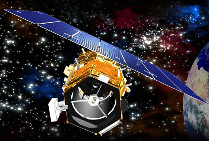
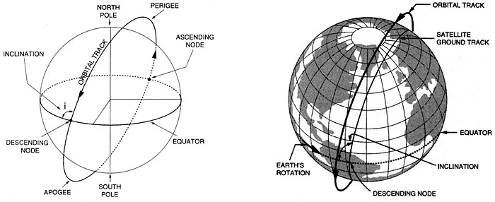
Satellites are placed at various heights and orbits to achieve desired coverage of the Earth's surface [11]. When the orbital speed exactly matches that of the Earth's rotation, the satellite stays above the same point at all times, in a geostationary [12] orbit. This is useful for communications and weather monitoring satellites Satellite platforms for electro-optical (E/O) imaging systems are usually placed in a sun-synchronous [13], low-earth orbit (LEO) so that images of a given place are always acquired at the same local time (Figure 2.02). The revisit time for a particular location is a function of the individual platform and sensor, but generally, it is on the order of several days to several weeks. While orbits are optimized for time of day, the satellite track may not always coincide with cloud-free conditions or specific vegetation conditions of interest to the end-user of the imagery. Therefore, it is not a given that usable imagery will be collected on every sensor pass over a given site
Aircraft often have a definite advantage because of their mobilization flexibility. They can be deployed wherever and whenever weather conditions are favorable. Clouds often appear and dissipate over a target over a period of several hours during a given day. Aircraft on site can respond with a moment's notice to take advantage of clear conditions, while satellites are locked into a schedule dictated by orbital parameters. Aircraft can also be deployed in small or large numbers, making it possible to collect imagery seamlessly over an entire county or state in a matter of days or weeks simply by having lots of planes in the air at the same time.
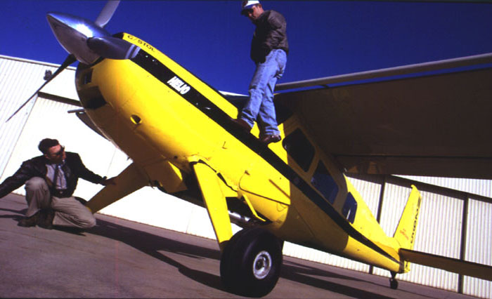
Aircraft platforms range from the very small, slow, and low flying (Figure 2.03), to twin-engine turboprop and small jets capable of flying at altitudes up to 35,000 feet. Unmanned platforms (UAVs) are becoming increasingly important, particularly in military and emergency response applications, both international and domestic. Flying height, airspeed, and range are critical factors in choosing an appropriate remote sensing platform, and you will learn about this in more detail later in the lesson. Modifications to the fuselage and power system to accommodate a remote sensing instrument and data storage system are often far more expensive than the cost of the aircraft itself. While the planes themselves are fairly common, choosing the right aircraft to invest in requires a firm understanding of the applications for which that aircraft is likely to be used over its lifetime.
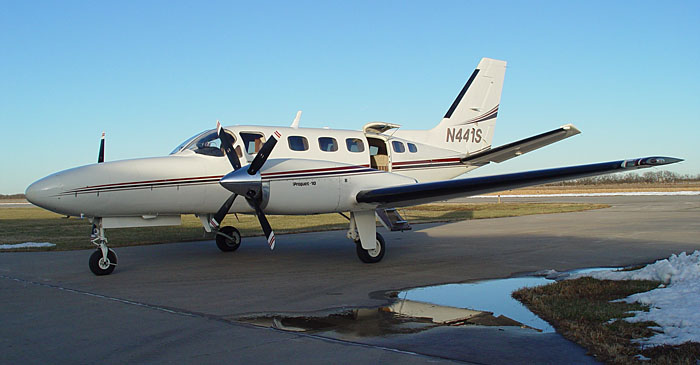
The scale and footprint of an aerial image is determined by the distance of the sensor from the ground; this distance is commonly referred to as the altitude above the mean terrain (AMT). The operating ceiling for an aircraft is defined in terms of altitude above mean sea level. It is important to remember this distinction when planning for a project in mountainous terrain. For example, the National Aerial Photography Program [14] (NAPP) and the National Agricultural Imagery Program [15] (NAIP) both call for imagery to be acquired from 20,000 feet AMT. In the western United States, this often requires flying much higher than 20,000 feet above mean sea level. A pressurized platform such as the Cessna Conquest (Figure 2.04) would be suitable for meeting these requirements.
With airborne systems, the flying height is determined on a project-by-project basis depending on the requirements for spatial resolution, GSD, and accuracy. The altitude of a satellite platform is fixed by the orbital considerations described above; scale and resolution of the imagery are determined by the sensor design. Medium-resolution satellites, such as Landsat, and high-resolution satellites, such as GeoEye, orbit at nearly the same altitude, but collect imagery at very different ground sample distance (GSD).
1 Sun-Synchronous Orbit. (2007, November 27). On Wikipedia, The free encyclopedia. Retrieved December 4, 2007, from http://en.wikipedia.org/wiki/Sun-synchronous_orbit [13]
Optical Sensors
In this lesson, you will be introduced to three types of optical sensors: airborne film mapping cameras, airborne digital mapping cameras, and satellite imaging systems. Each has particular characteristics, advantages, and disadvantages, but the principles of image acquisition and processing are largely the same, regardless of the sensor type. Lesson 3 will cover photogrammetric processing of data from these sensors to produce orthophotos [16] 1 and terrain models.
The size, or scale, of objects in a remotely sensed image varies with terrain elevation and with the tilt of the sensor with respect to the ground, as shown in Figure 2.05. Accurate measurements cannot be made from an image without rectification, the process of removing tilt and relief displacement. In order to use a rectified image as a map, it must also be georeferenced to a ground coordinate system.
If remotely sensed images are acquired such that there is overlap between them, then objects can be seen from multiple perspectives, creating a stereoscopic view, or stereomodel. A familiar application of this principle is the View-Master [17] 2 toy many of us played with as children. The apparent shift of an object against a background due to a change in the observer's position is called parallax [18] 3. Following the same principle as depth perception in human binocular vision, heights of objects and distances between them can be measured precisely from the degree of parallax in image space if the overlapping photos can be properly oriented with respect to each other; in other words, if the relative orientation is known (Figure 2.06).
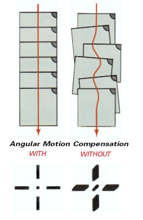
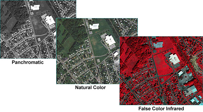
Airborne film cameras have been in use for decades. Black and white (panchromatic), natural color, and false color infrared aerial film can be chosen based on the intended use of the imagery; panchromatic provides the sharpest detail for precision mapping; natural color is the most popular for interpretation and general viewing; false color infrared is used for environmental applications. High-precision manufacturing of camera elements such as lens, body, and focal plane; rigorous camera calibration techniques; and continuous improvements in electronic controls have resulted in a mature technology capable of producing stable, geometrically well-defined, high-accuracy image products. Lens distortion can be measured precisely and modeled; image motion compensation mechanisms remove the blur caused by aircraft motion during exposure. Aerial film is developed using chemical processes and then scanned at resolutions as high as 3,000 dots per inch. In today's photogrammetric production environment, virtually all aerotriangulation, elevation, and feature extraction are performed in an all-digital work flow.
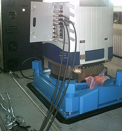
Figure 2.07 shows a Leica RC-30 aerial film camera. A hole is cut in the fuselage of the aircraft, and the camera is set in a gyro-stabilized mount as shown in Figure 2.08. This minimizes the effects of instantaneous aircraft motion and keeps the camera pointing perpendicular to the ground; the result is a sharper image and more controlled coverage from photo to photo (Figure 2.09).
In the United States, laboratory calibration of film aerial cameras is performed by the US Geological Survey, Optical Science Laboratory, in Reston, VA. If you are ever in that area, you can arrange for a visit to this unique and interesting facility; the services provided there have ensured the quality and accuracy of photogrammetrically-produced maps in the US for many decades. Most aerial survey projects require the aerial camera and lens to have been calibrated by the USGS no less than three years before the beginning of the project.
You can find a great number of USGS camera calibration certificates on the web in the Keystone Aerial Surveys Calibration Report [19] database. Camera systems are calibrated as a unique combination of camera body, lens, and film magazine. If you search the Keystone database for lens number 13366, for example, you should see the following result.
Table 3.01: Example Keystone database search results.
| Cam Num | Lens Num | CFL | Report Date | Lens Type | Platen | Report |
|---|---|---|---|---|---|---|
| 5325 | 13366 | 153.287 | 5/12/2000 | 6 | 707 | 5325-051200 |
| 5325 | 13366 | 153.301 | 10/1/2003 | 6 | 5325-707 | 5325-100103 |
| 5325 | 13366 | 153.298 | 10/30/2006 | 6 | 707 | 5325-103006 |
Lens 13366 has been calibrated 3 times, always with camera number 5325. When using the Keystone database, you can click on the report link for the most recent calibration to see the complete report. The camera is a Wild RC30 4; one of the most advanced and precise aerial film mapping cameras manufactured. Pay particular attention to the sections on
- calibrated focal length
- lens distortion
- lens resolving power (AWAR)
- principal points and fiducial coordinates.
Now look at the calibration report for lens number 13081, camera number 2961, and dated 1/5/2005. This is Wild RC10 camera manufactured in the 1980s, an early predecessor to the RC30. Compare the reports, particularly the values shown for AWAR. Mapping projects executed today often specify a minimum allowable AWAR for the camera lens.
Airborne digital mapping cameras have evolved over the past few years from prototype designs to mass-produced operationally stable systems. In many aspects, they provide superior performance to film cameras, dramatically reducing production time with increased spectral and radiometric resolution. Detail in shadows can be seen and mapped more accurately. Panchromatic, red, green, blue, and infrared bands are captured simultaneously so that multiple image products can be made from a single acquisition (Figure 2.10).
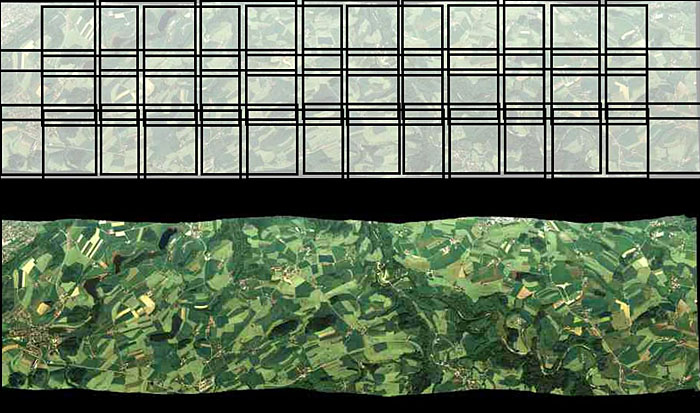
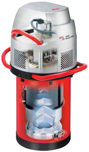
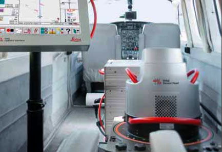
Digital camera designs are of two types: area arrays, and linear push-broom, or line-scanning, sensors. An area array camera, such as the Intergraph DMC (Figure 2.12) uses one or more two-dimensional charge-coupled device (CCD) arrays to create an image equivalent to a single frame image from an aerial film camera. The entire scene is imaged at the same moment in time, providing the same rigid geometric relationship for all points in the image with respect to each other. Coverage of an area of interest is provided with a block of overlapping photos, as shown in Figure 2.11. A push-broom sensor, such as the Leica ADS40 (Figure 2.13 and Figure 2.14), comprises multiple linear arrays, facing forward, down, and aft, which simultaneously capture along-track stereo coverage not in frame images, but in long continuous strips, or pixel carpets, made up of individual lines 1 pixel deep. Multiple linear CCD arrays capture panchromatic, near-infrared, red, green, and blue bands (Figure 2.15). Pointing the CCD arrays at aft, nadir, and forward viewing angles allows the sensor to capture multiple perspectives of the same point on the ground in a single pass, creating the stereo views required to extract elevation information (Figure 2.16).
Credit: R. Reulke, S. Becker, N. Haala, U. Tempelmann. “Determination and improvement of spatial resolution of the CCD-line-scanner system ADS40.” ISPRS Journal of Photogrammetry and Remote Sensing, Volume 60, Issue 2, 81-90. https://doi.org/10.1016/j.isprsjprs.2005.10.007 [20]
High-resolution satellite imagery is now available from a number of commercial sources, both foreign and domestic. The federal government regulates the minimum allowable GSD for commercial distribution, based largely on national security concerns; 0.6-meter GSD is currently available, with higher-resolution sensors being planned for the near future (McGlone, 2007). The image sensors are based on a linear push-broom design. Each sensor model is unique and contains proprietary design information; therefore, the sensor models are not distributed to commercial purchasers or users of the data. Through commercial contracts, these satellites provide imagery to NGA in support of geospatial intelligence activities around the globe.
Calibration of digital aerial cameras and satellite sensors is a much more complex process than calibration of a film camera. The digital sensor should be characterized for its radiometric response as well as for internal geometry. ASPRS and a number of federal government agencies have been working with sensor manufacturers to establish guidelines and procedures for sensor calibration and data product characterization. It is an ongoing effort, and standards are just beginning to emerge. The USGS Remote Sensing Technologies Project maintains a website with information on digital camera calibration [21] efforts, as well as collaborative efforts, such as the Interagency Digital Imagery Working Group [22] (IADIWG) and the Joint Agency Commercial Imagery Evaluation [23] (JACIE) group.
As digital aerial photography has matured, it has become integrated into many consumer-level, web-based applications, such as Google Earth and numerous navigation and routing packages. Microsoft has recently deployed a large number of aerial survey planes equipped with the Vexcel UltraCam sensor in an ambitious Global Ortho [24] program. Their goal is to provide very high-resolution color imagery over the entire land surface of the Earth, made publicly available through the Bing Maps platform. The following video (4:47) describes the data acquisition experience and process.
Video: Keystone Aerial Surveys: I Fly UltraCam (4:47)
[MUSIC PLAYING] We have 16 airplanes that we fly all over the United States. We have the largest fleet of aircraft totally dedicated to aircraft imagery collection in the United States, if not the world. Keystone purchased their first UltraCam in 2005. Keystone was in a situation where they had been collecting analog inventory for years, ever since the '60s. We identified that we had to go digital. We had to do it to survive. So our choice then was to pick out the right camera. There was a lot of competition from other companies, and we felt that to be state-of-the-art and to offer our clients what they needed, we chose UltraCam because of price point and what we considered quality and service that they provided.
If we had not upgraded to digital, specifically the UltraCam, we would have been considered a second class operator. We went from having one UltraCam-D to three UltraCam-X systems in only a matter of years. I think the real telling thing is once we have flown a project in digitally with our UltraCam, they don't want film anymore. Keystone's coming to a point where we're about to take our one millionth UltraCam frame. [MUSIC PLAYING] So here we are. The mount is green. We're about to take pictures here in about two seconds. And there's our first shot. I'm getting a quick view. An exact representation of the imagery that we are recording right now. So we'll go up on a four hour flight and at the end of it, I'm pretty certain that that imagery was good. Whereas, with film, you really don't know what's on it. You don't want to do a flight twice. So we're basically able to operate cheaper.
This spring was almost the tipping point. We were actually setting film cameras on the ground in our big season with people asking for digital imagery instead of the film imagery because of the quality. We had another client when we first delivered the digital imagery for them, they were able to read the serial number on a manhole cover. It's not just an image, there's so much more. Time, altitude, who flew it, camera serial numbers, the airplane it was installed in, the exact time of the photo, the sun angle of the photo. Basically, if you can type it, we can record it. The advantage of the UltraCam with its collecting all the bands allows us to do things with it that were not possible with an analog camera just using one film. We're collecting panchromatic, RGB color, and infrared at the same time. Infrared allows you to see wetland studies, impervious surface studies. Also [? distressed ?] foliage studies. You're dealing with nearly 14 bits. That 14 bits gives you the ability to see inside of shadows or fly under lower light conditions. With the X, we can now change cassettes in flight and really go all day long without having to land to download that.
They have three people on staff that, phone call away, they will either send us the parts or they'll be here to fix our camera. They have a service facility in Boulder where they can actually calibrate the camera. We chose to upgrade because Microsoft seems to have a very strong commitment to keeping their product up-to-date. Version 2.1 has some of our specific requests for reporting tools and better logging tools. The radiometry upgrades have also made it virtually a no-brainer to upgrade. The advantage that Vexcel has given us is the constant upgrades of these cameras. They're coming up with new inventions all the time. They had the D. Then they came up with the X. And now the XP. So when you have an UltraCam, you're basically buying into a product line that you will be able to use into the future. It's allowed Keystone to stay at the forefront of the profession in terms of offering the best equipment. UltraCam gives you beautiful, accurate imagery. It's reliable and has support that's second to none I'm Ken Potter from Keystone Aerial Surveys and I fly UltraCam.
1 Orthophoto. (2007, November 21). In Wikipedia, The free encyclopedia. Retrieved December 4, 2007, from http://en.wikipedia.org/wiki/Orthophoto [16]
2 View-Master (2007, November 9). In Wikipedia, The free encyclopedia. Retrieved December 5, 2007, http://en.wikipedia.org/wiki/View-master [17]
3 Parallax. (2007, 29 November). In Wikipedia, The free encyclopedia. Retrieved December 5, 2007, http://en.wikipedia.org/wiki/Parallax [18]
4 Wild was purchased by Leica Geosystems, which has since been incorporated into Hexagon. The camera referenced in this report is of the same type shown in Figure 7.
Lesson 3: Production of Digital Image Base Maps
Lesson 3 Introduction
Remote sensing, as a broad discipline within geospatial science, extracts two types of information from images: thematic (what is it?) and positional (where is it?). Thematic information is extracted through a process of image interpretation and analysis; positional information is extracted through the process of creating maps from remotely sensed data. In Lesson 2, we set the stage to discuss maps and mapping by providing a background in datums, coordinate systems, and georeferencing technology. In Lesson 3, we will begin to connect those concepts with the remotely sensed data itself, concentrating on the aerial photograph; however, we will see in later lessons how these principles are applied to elevation data.
Photogrammetry is defined as "the art, science, and technology of obtaining reliable information about physical objects and the environment through the process of recording, measuring, and interpreting photographic images and patterns of electromagnetic radiant energy and other phenomena. Photogrammetry provides the positional half of the information equation described above. In Lessons 3 - 5, we will concentrate on the photogrammetric principles of precise and accurate measurement that are essential to the creation of good base maps for GIS. In later lessons, we will introduce foundations of interpretation and image analysis that are also an important application of remote sensing. In this lesson, you will learn more about the special geometric relationships between overlapping aerial photographs, which allow creation of an accurate three-dimensional depiction of the ground. Odd as it may seem, we need this accurate three-dimensional model before a spatially accurate two-dimensional image base map (an orthophoto) can be generated. As was mentioned in Lesson 2, the third dimension, elevation, is needed in order to remove relief displacement from the source imagery.
This lesson will also introduce key elements of photogrammetric project planning, including constraints of lighting, weather, and season that apply to all types of passive optical sensors. You will be introduced to the techniques and methods of data extraction using specialized photogrammetric instruments and software, and you will learn to identify common image-based GIS data products. Finally you will use Internet data sources to find and download various types of aerial photography, and you will create an orthophoto base map using a raw aerial photo and a digital elevation model.
Lesson Objectives
At the end of this lesson, you will be able to:
- describe the basic photogrammetric concepts used in orthorectification of imagery.
- explain the difference between simple georeferencing and rigorous orthorectification.
- perform both simple georeferencing and rigorous orthorectification of both airborne and satellite imagery.
- use web-based tools to locate and download remotely sensed imagery.
- identify common image data formats and perform conversions from one format to another.
- overlay imagery data with vector data layer to prepare for visualization and analysis.
Questions?
If you have any questions now or at any point during this week, please feel free to post them to the Lesson 3 Questions and Comments Discussion Forum in Canvas.
Geometry of the Aerial Photograph
The Single Vertical Aerial Photograph
The geometry of an aerial photograph is based on the simple, fundamental condition of collinearity. By definition, three or more points that lie on the same line are said to be collinear. In photogrammetry, a single ray of light is the straight line; three fundamental points must always fall on this straight line: the imaged point on the ground, the focal point of the camera lens, and the image of the point on the film or imaging array of a digital camera, as shown in the figure below.
Picture the bundle of countless rays of light that make up a single aerial photograph or digital frame image at the instant of exposure. The length of each ray, from the focal point of the camera to the imaged point on the ground, is determined by the height of the camera lens above the ground and the elevation of that point on the ground. The length of each ray, from the focal point to the photographic image, is fixed by the focal length of the lens.
Now imagine that the camera focal plane is tilted with respect to the ground, due to the roll, pitch, and yaw of the aircraft. This will affect the length of each light ray in the bundle, and it will also affect the location of the image point in the 2-dimensional photograph. If we want to make precise measurements from the photograph and relate these measurements to real world distances, we must know the exact position and angular orientation of the photograph with respect to the ground. Today, we can actually measure position and angular orientation of the camera with respect to the ground with GPS/IMU direct georeferencing technology. But the early pioneers of photogrammetry did not have this advantage. Instead, they developed a mathematical process, based on the collinearity condition, which allowed them to compute the position and orientation of the photograph based on known points on the ground. This geometric relationship between the image and the ground is called exterior orientation. It is comprised of six mathematical elements: the x, y, and z position of the camera focal point and the three angles of rotation: omega (roll), phi (pitch), and kappa (yaw), with respect to the ground. The mathematical process of computing the exterior orientation of elements from known points on the ground is referred to by the photogrammetric term, space resection.
Refer again to the figure above. If we were together in a classroom, I could demonstrate the concept of space resection using my desktop and a photograph taken of my desktop from above. I could use pieces of string to represent individual rays of light; each string is of a fixed length based on the distance from the desktop to the camera when the photo was taken. You'll now have to try to picture this demonstration as I describe it in words. If you feel frustrated, imagine yourself as Laussedat trying to figure this out by himself back in the 1800s.
I attach one end of one piece of string to a particular point on my desktop, I attach the other end of the string to the image of that point on the photograph, and I pull the string taut. With that single piece of string, I cannot precisely locate or fix the position of the camera focal point or the orientation of the camera focal plane as it was when the photograph was taken. Now, I choose a second point, adding a second piece of string, and I pull both strings taut. I can't move the photograph around as much as I could with only one piece of string attached, but the photograph can still be rolled and twisted with respect to the desktop. If I identify yet a third point (that does not lie in a straight line with the first two) and attach a third piece of string, I now have a rigid solution; the geometric relationship between the desktop and the photograph is fixed, and I can locate the focal point of the camera in my desktop model. Adding more points adds to the strength of the geometric solution and minimizes the effects of any small errors I might have made, either cutting the string to its proper length or attaching the strings exactly to the points I identified. When we overdetermine a solution by adding additional, redundant measurements, we can make statistical calculations to quantify the precision of our geometric solution.
We don't have time in this course to go into the mathematics of analytical photogrammetry, but hopefully you can get a sense of it as a true measurement science. In fact, photogrammetry has traditionally been taught as a subdiscipline of civil engineering and surveying, rather than geography. Photogrammetry is not just about making neat and useful maps; a key function of the photogrammetrist, as a geospatial professional, is to make authoritative statements about the spatial precision and accuracy of photogrammetric measurements and mapping products. As you'll see in this lesson and the ones to come, you can easily be trained to push buttons in software to produce neat and interesting remote sensing products for use in GIS. It takes a more rigorous education to make quantitative statements about the spatial accuracy of those products. In my opinion, it is as much the duty of the photogrammetrist or GIS professional to make end users aware of the error contained in a data product as it is to give them the product in the first place. Understanding errors and the potential consequences of error is a very important part of the decision-making process. There's also a particular language used to articulate statements about error and accuracy. You will learn a little of this language in Lesson 6.
The Stereo Pair
Once the exterior orientation of a single vertical aerial photograph is solved, other points identified on the photographic image can be projected as more rays of light, more pieces of string, passing through the focal point of the camera and intersecting the target surface (the ground or my desktop). If the target surface is perfectly flat, then the elevations of the three known points determine a mathematical plane representing the entire surface. It is then possible to precisely locate any other point we can identify in the image on the target surface, merely by projecting a single, straight line. In reality, the target surface is never perfectly flat. We can project the ray of light from the image through the focal plane, but we can't determine the point at which it intersects the target surface unless we know the shape of the surface and the elevation of that point. In the context of our demonstration above, we need to know the exact length of the new piece of string to establish the location of the point of interest on the target surface. This is where the concept of stereoscopic measurement comes into play. If you are interested in learning more about the principles and history of stereoscopy, there is a long but very interesting YouTube video of a seminar with Brian May and Denis Pellerin titled, Stereoscopy: The Dawn of 3-D. Brian May and Denis Pellerin [26]. We've been able to build an entire science of measurement around something that is a natural, built-in, characteristic of the physical human being.
The advantage of stereo photography is that we can extract 3-dimensional information from it. Let's return to the example I described above. This time, imagine I have two photographs of my desktop taken from two separate vantage points, and that the individual images actually overlap. One image is taken from over the left side of my desk, and the other is taken from over the right side of my desk. The middle of my desktop can be seen in both photographs. Now, let's assume that we have established the exterior orientation parameters for each of the two photographs; so, we know exactly where they both were at the moment of exposure, relative to the desktop. We now have two bundles of light rays, some of them intersecting in the middle of my desktop. It is a fundamental postulate of geometry that if two lines intersect, their intersection is exactly one point. Voilà! Now we can precisely locate any point on the desktop surface, regardless of its shape, in 3-dimensional space. For any given point common to both photographs, we now know the exact length of each of the two pieces of string (one from each photograph) that connect to the imaged point on the ground. In photogrammetry, we call this a space intersection. If we have two photographs precisely oriented in space relative to each other, we can always intersect two lines to find the 3-dimensional ground coordinate of any point common to both photographs. The two photographs, oriented relatively to each other, are referred to as a stereo model.
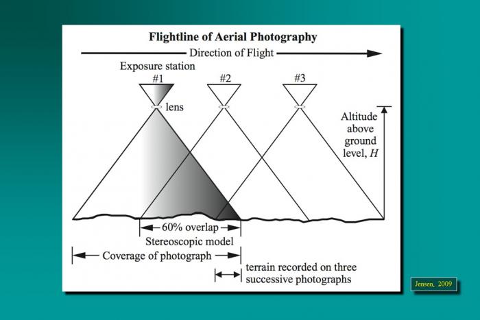
By extension, we could have a large block of aerial photographs, overlapping in the direction of flight as well as between adjacent flight lines, all oriented relatively to each other. This block, once constructed, represents all of the intersecting bundles of light rays from all of the overlapping photos. You can imagine that many of the points will be seen in a number of photographs. In fact, with 60% forward overlap, every point in a single flight line is seen 3 times. If the point falls in the 30% sidelap area between two flight lines, it will be seen 6 times; six rays will all intersect at one point. Actually, because some degree of measurement error is unavoidable, the intersection will occur within some sort of sphere, which represents the uncertainty in the projected coordinate of the point in question. As I mentioned earlier, the mathematical equations of photogrammetry allow us to quantify this uncertainty in statistical terms. Your readings will take you into greater depth and detail, but I hope my explanation helps you create a 3-dimensional picture in your mind, making the readings easier to understand.
Acquisition of Aerial Photography
For most photogrammetric mapping purposes, the goal is to image as much of the actual ground surface as possible. For this reason, it is customary to fly projects when deciduous trees are without leaves, when the ground is clear of snow and ice, when lakes and streams are within their normal banks, and when the sun is high overhead, minimizing shadows. In many parts of the world, this limits the optimal season for mapping to early spring, when days are getting long, but trees are relatively bare. Add the need for cloud-free skies to all these other requirements, and you can see why the flight operations of most photogrammetric mapping companies are not a big profit center. For any given location, there are a relatively small number of days per year when all the conditions are right for image acquisition.
By the way, these requirements are no different for space-based image acquisition. You already know that the orbits of passive imaging satellites are designed to follow local noon. That takes care of the time of day requirement. Add in all the other requirements, plus the constraints of orbital parameters and revisit times, and you can easily see why large-scale state and county mapping projects are still accomplished with aircraft. I'm sure we'll eventually see seamless coverage of states and nations with large-scale (1 meter/pixel GSD or better) satellite imagery, but it won't all be taken in the same season or even in the same year. Not until there are many, many more high-resolution imaging satellites circling the globe.
Sample Aerial Photography Specifications from Indiana Department of Transportation [27]
Aerial Imagery Guidelines from URISA Quick Study [28]
Several key computations related to flight planning are identified in these documents. These are:
- flight altitude above the ground required to achieve specified photo scale
- number of flightlines required to cover project area
- distance between (and total number of) flightlines required to achieve specified sidelap
- distance between (and total number of) successive exposures to achieve specified overlap
- total number of exposures required to complete project
In most aerial photography contracts, the aerial survey company provides a flight plan, based on customer specifications for scale and resolution, that enumerates all of the quantities outlined above along with a cost estimate based on those quantities.
Control and Georeferencing
The subject of control and georeferencing of a photogrammetric block could be the subject of several lessons in a course dedicated entirely to photogrammetry. I'm going to do my best to explain it conceptually without the math. Earlier in this lesson, you learned about the six parameters of exterior orientation that define the geometric relationship between an aerial photograph and the ground. I explained space resection and the way a minimum number of ground points can be used to solve the exterior orientation of a single vertical photograph. You may have thought to yourself how labor-intensive, expensive, and impractical it would be to actually solve the exterior orientation of each individual photograph in a large block by this method.
Photogrammetric mapping, based on very large blocks of hundreds or even thousands of aerial photographs, was made practical by the development of a technique called aerotriangulation, sometimes also called aerial triangulation, and often abbreviated as “A/T.” This short video from ASPRS [29] gives an overview of the concept, but a deep understanding comes from either years of training under a master, or a rigorous study of the mathematics. My reference to a master may sound a little overblown, but in my years of experience managing photogrammetric projects, a bad aerotriangulation solution that goes undetected is one of the most costly and time-consuming problems to correct. A/T is usually performed by the most experienced photogrammetrist in the organization, and there simply aren't that many true experts in it, perhaps a thousand or two at most worldwide. There are many software programs available to compute an A/T adjustment, but it’s easier to get a bad result than a good one, especially if the person designing the block and evaluating the statistical results doesn't have a deep theoretical understanding combined with a lot of practical experience.
The easiest way I have found to simply explain the concept of aerotriangulation is an extension of my desktop analogy. Picture again the bundles of intersecting rays generated by two overlapping photographs; the figure below depicts 3 photos in a single flight line. Now extend that picture in your mind's eye to include a second flight line "side-lapping" the first, also imaging points A, D, and G on the ground.
Point D, for example, is seen from 3 perspectives in the first flight line, and from another 3 perspectives in the side-lapping flight line I've asked you to visualize. Imagine that both flight lines continue on with many more end-lapping photos. All points common to adjacent flight lines, such as points D, G, and beyond, are going to be viewed with 6 intersecting rays. Even if we did not have a ground coordinate for every single one of these "tie points," you can imagine that, by enforcing the condition that the 6 rays must precisely intersect, there is still a lot of geometric stability in the block. This is the basic premise of aerotriangulation: enforcing the collinearity condition and the redundant intersection of image rays in "object space" creates a bridge from one photo to the next, thereby reducing the amount of ground control needed to reconstruct the exterior orientation for every photo.
If GPS/IMU direct georeferencing is available, the effect is to add additional control at each of the camera focal points, the photo centers, as they are often called. Remember that direct georeferencing gives us the 6 parameters of exterior orientation for every photo. We can use the direct georeferencing measurements as the first approximation of the aerotriangulation solution, and we no longer need actual ground control points. The GPS/IMU measurements for each photo center will inevitably contain errors, but we can reduce the impact of these errors in subsequent iterations of the block adjustment computation, simply by enforcing ray intersection for all the image tie points. This is done mathematically for all photos in the entire block simultaneously, and the A/T results give the photogrammetrist a quantitative assessment of the "goodness of fit" for this system of many redundant observations.
Photogrammetric Data Collection
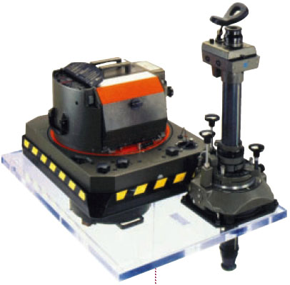
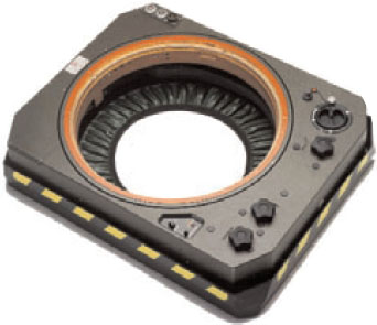
Stereoplotters and Photogrammetric Workstations
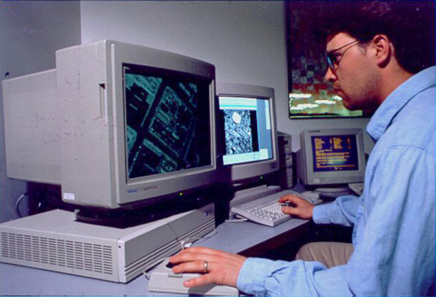
A stereoplotter is an instrument that can be used to recreate stereo models, so that a 3-dimensional model of the ground can be viewed, measured, and mapped by an operator. Compare the historical stereoplotters in the Lesson 1 reading to the softcopy workstation shown below. Binoculars have been replaced with other, less restrictive, forms of 3-dimensional viewing. In the example below, the glasses worn by the operator are polarized so that his right eye is seeing one image of the stereo pair, and his left eye is seeing the other.
Feature and Elevation Collection
Prior to the advent of digital workstations, map features were scribed by photogrammetric technicians on a drawing table integrated into the stereoplotter apparatus, often employing a pantograph [30] to enlarge the drawing to the final, desired map scale. Skilled cartographers would then use colored inks on semi-transparent materials, such as mylar, to create master map sheets that could be reproduced by blueprint or photo offset processes. These cartographers would add labeling and annotation as required. The final map was as much a work of art as it was a feat of technology. Today, feature data can be easily captured as 2-dimensional or 3-dimensional points, lines, and polygons when a Computer Aided Design (CAD) or GIS system is integrated into the softcopy workstation. Points might describe the location of fire hydrants, light poles, or simple building locations; lines could represent road or stream edges and centerlines; polygons are often used to represent detailed building footprints, stands of vegetation, water bodies, etc. In either a CAD or GIS package, each feature can be collected with unique line styles, line weights, and colors. If GIS software is used, the operator can also collect attribute information, such as road surface material, or building type, insofar as he can interpret this information from the aerial photograph.
Elevation data can be captured in a variety of ways; as in the case of feature data, methods have evolved along with photogrammetric technology. The earliest method for collecting elevation data was to manually draw isolines of elevation, or contours. It requires a great amount of skill and experience for an operator to draw spatially accurate, aesthetically pleasing contours. Contours are still one of the most effective representations of 3-dimensional topography on a 2-dimensional map; they are laborious to draw by hand, and while they can be generated automatically in a number of software packages, it usually requires a lot of manual editing to smooth jagged lines, to remove small artifacts, and to add labels. Many engineers learned to use contours early in their careers and still prefer them to other more modern, automated forms of digital elevation data.
Profiling is a technique of elevation data capture that was used extensively by the USGS and many private firms to create elevation data intended for input into the orthorectification of imagery. In this method, the stereoplotter is set to automatically drive the digitizing mark in evenly spaced profiles running the length or width of the stereo model. The operator's job is to keep reading elevations as accurately as possible in this dynamic environment; the stereo plotter automatically records elevations at regular intervals. The end result is a grid of regularly spaced points, which may or may not correspond to interesting or significant features of the actual terrain. This method of profiling works best in flat areas and in applications where accuracy and detail are not required. It was used quite a bit in the early days of orthophoto production, but is less common today.
Most elevation data derived from photogrammetry today is captured as randomly spaced mass points and breaklines. The photogrammetric technician collects individual 3-dimensional points at whatever frequency and in whatever pattern he deems appropriate to represent the ground surface. In addition, important linear features, such as road edges, curbs, walls, ridges, drains, etc., are captured as 3-dimensional lines. The mass points and breaklines are combined using surface modeling software to create a triangulated irregular network, or TIN. These elevation data products will be explained in more detail in the next lesson.
Image Data Products
Orthophotos
The term orthorectification refers to the process that removes effects of relief displacement, optical distortions from the sensor, and geometric perspective from a photograph or digital image. In a normal photograph, objects closer to the camera appear larger than objects of equal size that are further away from the camera. This presents an obvious difficulty in measuring objects accurately or determining their precise location in a reference coordinate system. In order to use perspective imagery as a map or in a geographic information system (GIS) environment, these geometric distortions must be corrected. The resulting image is referred to as an orthophoto or orthoimage.
Orthoimages can be created from any perspective image, regardless of the source, as long as three things are known:
- interior orientation, which describes the internal geometry of the camera system;
- exterior orientation, which describes the geometric relationship between the image and the ground;
- shape of the ground surface, which must be known in order to remove the effects of relief displacement. A digital terrain model must be supplied as input to the orthorectification process, in addition to the internal and external sensor geometry described above.
Returning to our familiar desktop example, the orthoimage is what would result if we took the 3-dimensional model created by all the intersecting light rays and projected every point straight down from the ground surface to an arbitrary flat plane. Each point would be in its appropriate planimetric (x, y) location, and all the effects of relief would be removed. The resulting image would have the exact same scale everywhere.
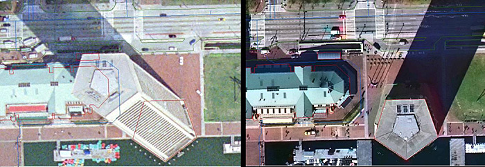
An orthophoto created using an elevation model representing only the bare ground surface will exhibit building lean everywhere except directly below the vantage point of the camera. All USGS and USDA orthophotos are created this way, as are the vast majority of state, county, and municipal orthophotos. On page 188 of Jensen (2007), he shows a comparison of this type of ground orthophoto to a true orthophoto, one which was created using a surface model comprising all of the above ground features at their proper elevation. True orthophotos are preferable in dense urban areas where the lean of tall buildings would obscure many important features on the ground between buildings. Building lean is also very distracting to GIS users, when they overlay building footprint data on top of an orthophoto backdrop. In a true orthophoto, the building footprints will line up with the images of the rooftops; in a ground orthophoto, they will not. Even though both datasets may be equally accurate and correct, the map still doesn't "look right."
Orthophoto Product Specifications
The specification for a digital orthophoto product deliverable must stipulate a ground coordinate system, pixel dimensions, spatial accuracy requirements, and the image file format. These specification elements are usually driven by the end user's application.
Many GIS systems today allow for reprojection of coordinate systems on-the-fly. However, when a raster image such as an orthophoto is projected from one coordinate system to another, it often requires resampling of the pixels, which can degrade the image quality and introduce artifacts. It is also computationally intensive, and can be quite time-consuming if the project includes a large number of high-resolution images. It is usually preferable to have the orthorectification process output orthoimagery in the coordinate system the end user intends to use for analysis. If there are multiple end users with diverse applications, which is often the case, a discussion and agreement on an output coordinate system should be part of the initial project design.
The size of the output pixel must be defined before running the orthorectification process. Knowing the output coordinate system before defining the pixel size is helpful; if one will be working in feet, it is preferable to have pixels defined as a round number interval, such as 1 foot, or 0.5 feet. Likewise for a metric coordinate system, pixel sizes of 1 meter, 50 cm, 30 cm or 25 cm are common. Finally, the GSD of the raw imagery should be considered; there is no point to creating an orthoimage with 25 cm pixels from an input image with a nominal GSD of 1 meter. It is customary to choose an output pixel size slightly larger than the nominal GSD of the input image; for example, if the output pixel size desired is 1 meter, then the project is usually designed for acquisition of data at a nominal GSD of slightly less than 1 meter, such as .8 or .9. This allows for the variation of actual GSD during acquisition due to perspective and relief, as described above, without compromising the spatial resolution of the end product.
Spatial accuracy of the end product depends on the quality of the georeferencing, either as inferred from ground control or provided by direct georeferencing technology. Spatial accuracy and pixel size (GSD) are completely unrelated. The size of a pixel has no physical bearing on the accuracy of its location in the ground coordinate system. However, in practice, it is customary when circumstances permit, to specify a spatial accuracy requirement that is comparable to the size of a pixel in ground units. For example, if the specified pixel size is 1 foot, then the spatial accuracy requirement might be defined such that each 1-foot pixel in the image was assured to be within 1 or 2 feet of its "true" location in the ground coordinate system. This is the ideal. In practice, depending on the end user application, it is not always possible or necessary to follow this rule. If the primary purpose of the imagery is simply to identify objects and measure their size relative to each other, then the absolute spatial accuracy in terms of ground coordinates may be less important. But generally, the rule of thumb is to target a root-mean-square-error (RMSE) for spatial accuracy equivalent to the size of a pixel in the output image. It should be noted, in case it is not already clear, that an orthoimage only has a spatial accuracy component in the horizontal. There is no elevation component to the orthoimage; it is strictly a 2-dimensional product, even though a 3-dimensional terrain model was required in order to produce it.
Image Data Formats
Image data are rasters, stored in a rectangular matrix of rows and columns. Radiometric resolution determines how many gradations of brightness can be stored for each cell (pixel) in the matrix; 8-bit resolution, where each pixel contains an integer value from 0 to 255, is most common. Modern sensors often collect data at higher resolution, and advanced image processing software can make use of these values for analysis. The human eye cannot detect very small differences in brightness, and most GIS software can only read an 8-bit value.
In a grayscale image, 0 = black and 255 = white; and there is just one 8-bit value for each pixel. However, in a natural color image, there is an 8-bit value for red, an 8-bit brightness value for green, and an 8-bit value for blue. Therefore, each pixel in a color image requires 3 separate values to be stored in the file. There are three possible ways to organize these values in a raster file.
- BIP - Band Interleaved by Pixel: The red value for the first pixel is written to the file, followed by the green value for that pixel, followed by the blue value for that pixel, and so on for all the pixels in the image.
- BIL - Band Interleaved by Line: All of the red values for the first row of pixels are written to the file, followed by all of the green values for that row followed by all the blue values for that row, and so on for every row of pixels in the image.
- BSQ - Band Sequential: All of the red values for the entire image are written to the file, followed by all of the green values for the entire image, followed by all the blue values for the entire image.
Orthoimages are delivered in a variety of image formats, compressed and uncompressed. The most common are TIF and JPG. Compression eases data management challenges, as large high-resolution orthophoto projects can easily result in terabytes of uncompressed imagery. Compression can also speed display in GIS systems. The downside is that compression can introduce artifacts and change pixel values, possibly hampering interpretation and analysis, particularly with respect to fine detail. The decision to compress should be driven by end user requirements; it is not uncommon to deliver a set of uncompressed imagery for archival and special applications along with a set of compressed imagery for easy use by large numbers of users. If there is an intention for web-based display or distribution of orthoimagery, a compressed set of orthoimagery is often recommended. In any event, georeferencing information must also be provided. Both TIF and JPG image formats can accommodate georeferencing information, either imbedded in the image file itself, as in the case of GeoTIF, or as a separate file for each image, as in the case of TIF with a TFW (TIF World) file. The georeferencing information tells GIS software 1) the size of a pixel, 2) where to place one corner of the image in the real world, and 3) whether the image is rotated with respect to the ground coordinate system.
Other popular image formats you may encounter are:
- ECW [31]: developed by ERMapper, now owned by ERDAS. Uses wavelet compression to reduce file size.
- GRID [32]: developed by Esri; supported by some remote sensing software packages, but not as common as other formats.
- IMG [33]: developed by ERDAS for Imagine; supported by many GIS and remote sensing software packages.
- JP2 [34]: JPEG 2000, developed by JPEG group. Widely supported by most GIS and remote sensing software packages.
- SID [35]: MrSid, developed by Lizard Tech. Uses wavelet compression to reduce file size. Read by many software packages, but requires proprietary software license to create.
Lesson 4: Production of Digital Elevation Models
Lesson 4 Introduction
In this lesson, we will also continue the discussion of elevation data in more depth, including many additional forms and formats for the representation of terrain as a base map layer. Photogrammetry was historically the primary approach to elevation data creation; in recent years, technologies such as lidar and IFSAR have surpassed photogrammetric methods for large area collection. We won't have time to discuss the design and operation of those technologies (they are covered in other courses in the remote sensing curriculum); but, we will discuss the elevation products that are generated from all remote sensing technologies.
We will also continue the discussion of specifications and standards; in this case, focusing on those that drive elevation data development at the federal, state, and county level in the United States. This, and the discussion of orthophoto standards, will set the stage for a discussion of data validation, accuracy assessment, and quality assurance/quality control methods which are a critical part of the overall base mapping mission.
Lesson Objectives
At the end of this lesson, you will be able to:
- describe the basic photogrammetric concepts used in creation of digital elevation models;
- explain the characteristics of, and processing methods used to produce, digital elevation models, digital terrain models, digital surface models, and topographic contours;
- discuss the strengths and weaknesses of various types of terrain representation in GIS analysis and applications;
- identify common artifacts and anomalies that occur in elevation data and methods used to correct them;
- identify common elevation data formats and perform conversions from one format to another;
- overlay elevation data with imagery and vector data to prepare for visualization and analysis.
Questions?
If you have any questions now or at any point during this week, please feel free to post them to the Lesson 4 Questions and Comments Discussion Forum in Canvas.
Elevation Data Collection
The geometric conditions of a pair of overlapping photographs, coupled with the evolution of stereo vision in most creatures that inhabit our planet, made photogrammetry the most important method for topographic mapping for over a century. For decades, topographic maps have been irreplaceable planning and design tools for the military, for civil engineers, for scientists, and even for the adventuring public. The depiction and interpretation of terrain data from a 2-dimensional paper product required special skills and considerable practice. While this type of depiction was incredibly useful and enabled many great accomplishments, advances in computer graphics, animation, and 3D rendering in the past few decades are quickly turning the 2D topographic map into a quaint historical relic.
Historically, elevation data was almost always collected as a "bare-earth" model, eliminating above ground features such as buildings, vegetation, and bridges. Today, because many applications make use of the above-ground features, digital surface models which include these features are often specified as additional deliverables.
Stereo aerial photography or satellite imagery is still a very important source of elevation data. Human beings drawing cartographically-pleasing contours by hand is rare in today's mapping industry, but it is still common to manually extract elevation points (mass points) and breaklines along key features of the natural and man-made landscape. Automated image correlation techniques are also useful, although there is almost always a need for manual editing and correction if a clean bare ground surface is desired. Autocorrelation is a fast and effective way of producing digital surface models, particularly for the generation of "true orthophotos." which were discussed in Lesson 3.
Active remote sensing technologies, particularly lidar [36]and IFSAR [37], are quickly gaining acceptance as the most accurate and/or cost-effective ways to collect high-resolution elevation data over large areas. An in-depth discussion of either of these technologies (including sensor design and operation, project planning, data processing, and product generation) is beyond the scope of this course. However, the textbook readings do describe these technologies at an overview level. Most of the information in this lesson, which deals with the elevation data products, rather than the method of acquisition, is applicable regardless of the sensor used for acquisition.
Seamless coverage of the United States with current digital orthophotography has been achieved, and is kept current, by a combination of government and commercial activities. In previous lessons, we discussed federal programs, such as USGS and USDA, and commercial endeavors such as the Microsoft/Bing Global Ortho Project. The USGS has developed and maintained seamless elevation data coverage of the United States through the National Elevation Database, but much of the source information for the NED is very old and of relatively low accuracy and resolution. There is significant interest in upgrading the nationwide elevation coverage with high-resolution, high-accuracy data, but it would require commitment of hundreds of millions of dollars for data acquisition and processing. One of the best cost-benefit arguments for seamless elevation data appears to be in support of FEMAs floodplain mapping program, but the pool of potential users of this data is much larger. Execution of a national elevation mapping program will require a significant number of interagency partnerships and cooperative cost-sharing agreements.
The viability of various remote sensing technologies for creation of a seamless national elevation database was the subject of a National Academies of Science report published in 2007. The study was done for FEMA, and the committee was made up of experts in mapping as well as engineering applications. This report, Elevation Data for Floodplain Mapping [38], can be downloaded for free and provides an in-depth comparison of photogrammetry, lidar, and IFSAR that should more than satisfy the student who would like to read beyond the scope of the assigned reading in this course.
Elevation Data Products
Elevation Data Product Types
A terrain surface can be characterized in many ways depending on the interest and perspective of the end user. This unit provides definitions for the types of terrain models most commonly encountered for mapping and GIS applications.
Digital Elevation Model (DEM)
A digital elevation model (DEM) contains elevations at points arranged in a raster data structure, a regularly spaced x, y grid, where the intervals of Δx and Δy are normally in linear units (feet or meters) or geographic units (degrees or fractions of degrees of latitude or longitude). The z-values in a DEM represent the height of the terrain, relative to a specific vertical datum and void of vegetation or manmade structures such as buildings, bridges, walls, et cetera. The elevation of lakes and rivers in a DEM implies the height of the water surface based on the elevation of the exposed shoreline. The observations, or direct measurements, of elevation that comprise the DEM are almost never actually captured on a regular grid; therefore, the elevation for any given point in the grid is normally interpolated from other forms of source data. Lidar, for example, yields a dense set of irregularly spaced points; interpolation to a grid requires using one of many possible interpolation algorithms, which produce varying results. Linear features, such as streams, drainage ditches, ridges, and roads, are often lost in a DEM if the grid spacing is larger than the dimensions of the feature. Furthermore, in a DEM, it is unlikely that the sharp edge of the feature will be represented correctly in the terrain model. The DEM, because it is a raster data structure similar to a digital image, is an efficient format for storage, analysis, rendering, and visualization.
Digital Terrain Model (DTM)
A digital terrain model (DTM) data structure is also made up of x,y points with z-values representing elevations, but unlike the DEM, these may be irregularly or randomly spaced mass points. Direct observations of elevation at a particular location can be incorporated without interpolation, and the density of points can be adjusted so as best to characterize the actual terrain. Fewer points can describe very flat or evenly sloping ground; more points can be captured to describe very complicated terrain. In addition to mass points, the DTM data structure often incorporates breaklines (further defined below) to retain abrupt linear features in the model. A DTM is often more expensive and time-consuming to collect than a DEM, but is considered technically superior for most engineering analyses because it retains natural features of the terrain.
Digital Surface Model (DSM)
A digital surface model (DSM) includes features above the ground, such as buildings and vegetation, and is used to distinguish a bare-earth elevation model from a non-bare-earth elevation model. The term DSM is generally applied regardless of whether the data are in gridded format (as in the DEM defined above) or mass point format (as in the DTM defined above).
Triangulated Irregular Network (TIN)
A triangulated irregular network (TIN) represents terrain with adjacent, non-overlapping triangular surfaces. A TIN is a vector data structure generated from the mass points and breaklines in a DTM. TINs also preserve abrupt linear features and are excellent for calculations of slope, aspect, and surface area and for automated generation of topographic contours, which are all important functions to the flood study engineering. Storage formats for TINs are more complex than either DEMs or DTMs, because the relationship of elevation points and triangular surfaces must be preserved within the data structure.
Breaklines
Breaklines are linear data structures that represent a distinct or abrupt change in the terrain. They comprise a series of vertices with z-values (elevations) attached. Breaklines contained in a DTM will be forced as edges in a TIN model. Breaklines are usually stored in separate files, as lines with 3-dimensional vertices, in a variety of common CAD or GIS file formats.
Contours
Contours are isolines of elevation; they are the traditional method for representing a three-dimensional surface on a two-dimensional map. They are excellent for human interpretation, but inferior to DEMs, DTMs, and TINs for computer display and analysis. Historically, contours were drawn by hand and smoothed to produce a cartographically pleasing product. Now, automated methods for producing contours from TINs or DEMs are available, but the final product contains no new information and adds little value to an engineering analysis. Contours are usually stored as two-dimensional lines, with an attribute or label containing the appropriate elevation value.
Elevation Data Product Specifications
Data product specifications for terrain models normally include a vertical accuracy requirement and some indication of the desired density of x, y, z points used to create the terrain models. For a DEM, the post-spacing is defined by the distance between points on the elevation grid. As with imagery, it makes little sense to define a DEM post spacing that is denser than the nominal point spacing of the source data. Based on the end user application, the data acquisition specification should ensure that the nominal point spacing, or ground sample distance, exceeds the post spacing required for the final deliverable product.
Specifications for breaklines usually adhere to the same vertical accuracy requirement defined for the mass points, and, in addition, stipulate which linear features are to be collected (i.e., road centerlines and/or edges, water body centerlines and/or edges, berms, levees, retaining walls, etc.).
Contour data products are specified by the desired contour interval; for example, a 5-foot contour dataset would contain a set of isolines at elevations of 0 feet, 5 feet, 10 feet, 15 feet, etc. The contour interval is usually chosen to represent as much terrain detail as possible without making the map or visual display overly crowded or cluttered; flatter areas will usually have smaller contour intervals, and hilly areas will usually be represented with larger contour intervals. If the terrain over the study area varies greatly, it may be difficult to arrive at one optimal contour interval for the entire project.
Elevation Data Formats
As you have seen, there are a number of inherently different ways of representing elevation data: grids, points, TINS, contours, etc. For each one of these data types, there are multiple file formats that can be used to save and exchange them.
Point Cloud
Elevation data can be a simple collection of XYZ points, often called a point cloud when the points are numerous and very densely spaced, as with lidar data. Point data is conceptually simple; however, it is often advantageous to attach a large number of attributes to each point, in which case, the file structure can become very cumbersome very quickly. ASCII and SHP work for small datasets, but are very inefficient for large numbers of attributed points.
- ASCII
- Esri SHP
- LAS - a binary point-based data format, maintained by ASPRS, designed specifically for lidar datasets contains millions of points with numerous attributes.
Digital Elevation Model (DEM)
A DEM is a raster, just like an optical image, so it can be stored in many of the common image formats described in Lesson 4. The important difference is that each cell in an image raster usually contains a discrete integer value (for example, in an 8-bit image, each cell contains an integer value from 0 - 255), whereas elevation values are continuous and can be expressed with decimal places appropriate for the accuracy of the data. Elevation rasters, therefore, are defined to store floating point [40] values rather than integers.
Commonly encountered raster elevation formats, previously described as image formats, are:
- TIF and GeoTIF
- IMG
- Esri GRID
- SID - While it is possible to store elevation data in the compressed SID format, I have honestly never been given one or seen SID format specified as a deliverable in a civilian or commercial project. One would want to be careful about using compression on a DEM, because any alteration to the original pixel value (in lossy compression) would affect the spatial accuracy of the dataset and could potentially change the results of spatial analysis.
Common raster formats specifically designed for elevation data only are:
Both of these formats are used for specific data products that meet USGS or NGA product standards; post-spacing, accuracy, and collection methods are prescribed in addition to the format of the file itself. These formats are only used for these USGS and NGA products; they are not generally used for more generic elevation datasets.
Digital Terrain Model (DTM)
A digital terrain model consists of 3D points and 3D breaklines. There are a number of CAD data formats, such as AutoCAD DXF and Microstation DGN, which hold both point and line data in a single file. This is less common in GIS, where files are normally restricted to one type: either point, line, or polygon. Geodatabases can contain multiple feature classes to accommodate these multiple topologies.
Digital Surface Model (DSM)
A DSM is a special case of either a point cloud, a DEM, or a DTM; the difference is whether the elevation surface represented is bare ground or if it contains above ground features. Data formats used for DSMs are the same as for point clouds, DEMs, and DTMs described above.
Triangulated Irregular Network (TIN)
TINs are an efficient representation of terrain for visualization and analysis, but they are most efficiently used when generated on-the-fly and stored in random access memory (RAM). Points, DEMs, and DTMs can all be used to generate TINs, and there are many different TIN generating algorithms and data formats; some are open source but many are proprietary. It is quite uncommon to see a TIN specified as a deliverable product; therefore no specific TIN formats are presented here.
Breaklines
Breaklines are 3D lines, and they can be represented in any number of common 3D polyline formats, such as:
- DXF
- DGN
- SHP
Contours
Contours are isolines of elevation; a single contour line has the same elevation value everywhere. Historically, contours were often stored as 2D lines, with the elevation added as an attribute or label. That approach makes it very difficult to do any kind of 3D analysis on a contour layer; therefore, it is most common today to find contours in the same 3D polyline formats described above for breaklines.
Lesson 5: Management of Imagery and Elevation Data
Lesson 5 Introduction
Lesson Objectives
At the end of this lesson, you will be able to:
- describe methods used to store and manage large image data and terrain data sets for multiple, distributed users;
- discover, download, and import a variety of imagery and elevation datasets from federal, state, and local public domain sources;
- discuss the strengths and limitations of web services vs. local hosting for both imagery and elevation datasets.
Questions?
If you have any questions now or at any point during this week, please feel free to post them to the Lesson 5 Questions and Comments Discussion Forum in Canvas.
Lesson 6: Validation of Imagery and Elevation Data
Lesson 6 Introduction
Lesson 6 provides an overview of accuracy assessment procedures and standards applied to remotely sensed mapping datasets intended for public use in the United States. In the context of this lesson, accuracy assessment refers primarily to geometric fidelity of the dataset, the degree to which the spatial coordinates of a data element agree with their “true” coordinates on the earth’s surface. However, in reference to image analysis, accuracy assessment also refers to the correctness of the thematic maps produced by land cover classification or change detection. Geometric accuracy is the focus of this lesson; classification accuracy is discussed in depth in Geography 883.
Accuracy assessment is a quantitative analysis of the spatial correctness of the dataset compared to the surface it represents. For most mapping products, there are also aesthetic standards for elements of quality which may not affect spatial accuracy, but can either enhance or detract from the experience of viewing the data or using it as a backdrop in GIS. The lesson material will focus on quantitative methods of accuracy assessment, but, for completeness, will also touch upon the qualitative. Together, the quantitative and qualitative evaluations are referred to by the broader terms, quality assurance and quality control (QA/QC).
A number of accuracy standards, used by public agencies and many private entities throughout the United States, will be presented in the textbook readings and summarized in the online course material. The study of standards and data specifications demands concern for minute details and precise use of terms and definitions. In this course, we have not been able to study all of the detailed elements of remote sensing technology and datasets addressed by most mapping standards; therefore, it’s important to try to get an overall sense of the major categories of issues being addressed. By the end of this lesson, the student should have an appreciation for the way remote sensing datasets are evaluated for geometric accuracy, and the way the results of those evaluations are (or at least, should be) reported to end users.
Lesson Objectives
At the end of this lesson, you will be able to:
- describe and compare various federal and state standards for imagery and elevation data;
- compute a quantitative accuracy assessment in accordance with FGDC standards;
- perform visual quality assessment for both imagery and elevation data.
Questions?
If you have any questions now or at any point during this week, please feel free to post them to the Lesson 6 Questions and Comments Discussion Forum in Canvas.
Definitions
The terms quality control and quality assurance are often used somewhat interchangeably, or in tandem, to refer to a multitude of tasks performed internally by the data producer and externally, or independently, by the data purchaser. For the purposes of this course, we will adopt the following definitions provided in Maune (2007):
Quality Assurance (QA) –
Steps taken: (1) to ensure the end client receives the quality products it pays for, consistent with the Scope of Work, and/or (2) to ensure an organization’s Quality Program works effectively. Quality Programs include quality control procedures for specific products as well as overall Quality Plans that typically mandate an organization’s communication procedures, document and data control procedures, quality audit procedures, and training programs necessary for delivery of quality products and services.
Quality Control (QC) –
Steps taken by data producers to ensure delivery of products that satisfy standards, guidelines, and specifications identified in the Scope of Work. These steps typically include production flow charts with built-in procedures to ensure quality at each step of the work flow, in-process quality reviews, and/or final quality inspections prior to delivery of products to a client.
Independent QA/QC –
Steps taken by a QA/QC specialty firm, hired by the client (e.g., government or data producer) to independently validate the effectiveness of the data producer’s quality processes.
Quantitative accuracy assessment (testing remotely sensing mapping products against ground control checkpoints) falls under the category of independent QA/QC defined above. It is normally conducted by an individual or organization that had no involvement in the data acquisition or production. The ground check points are not made available to the data producer; so that the final coordinate comparison is truly an independent test of spatial accuracy.
Before we delve further into the topic of accuracy assessment, we must define exactly what we mean when we use the term "accuracy" and distinguish it from the related term, "precision."
Absolute accuracy -
Absolute accuracy is the closeness of an estimated, measured, or computed value to a standard, accepted, or true value of a particular quantity. In mapping, a statement of absolute accuracy is made with respect to a datum, which is, in fact, also an adjustment of many measurements and has some inherent error. The statement of absolute accuracy is made with respect to this reference surface, assuming it is the true value.
Relative accuracy -
Relative accuracy is an evaluation of the amount of error in determining the location of one point or feature with respect to another. For example, the difference in elevation between two points on the earth's surface may be measured very accurately, but the stated elevations of both points with respect to the reference datum could contain a large error. In this case, the relative accuracy of the point elevations is high, but the absolute accuracy is low.
Precision -
Precision is a statistical measure of the tendency for independent, repeated measurements of a value to produce the same result. A measurement can be highly repeatable, therefore very precise, but inaccurate if the measuring instrument is not calibrated correctly. The same error would be repeated precisely in every measurement, but none of the measurements would be accurate.
Independent check points are used to assess the absolute accuracy of a remotely-sensed dataset. Realize, however, that the check point coordinates are also derived from some form of surveying measurement, and there is also some degree of error associated with them. It is customary to require that the check points be at least three times as accurate as the targeted accuracy of the mapping product being tested; for example, if an orthophoto product is specified to have no more than 1 foot of horizontal error, then the check points used to test the orthophoto product should themselves contain no more than 1/3 foot of error.
As you will learn in this lesson, quantification of error and accuracy relies on statistical principles of probability. Accuracy standards for imagery and terrain data are described in probabilistic terms; for example, one might report that the coordinates of an object derived from an orthophoto image were tested against independent ground checkpoints and were shown to agree within certain number of feet at the 90% or 95% percent confidence level. Confidence level refers to the probability that any other independently tested point in the dataset will differ from its true value by no more than the stated amount.
The statistical model used to determine this confidence level is most often the normal, or Gaussian, distribution [43]. The assumption underlying the use of this statistical model is that the errors associated with repeated measurements of the same physical quantity will distribute themselves according to a particular probability density function, the Gaussian "bell curve," shown below in Figure 1. Measurements very close to the true value are the most likely, but measurements that deviate from the true value will occur on a less frequent, yet predictable, basis. The peak of the bell curve represents the mean of all measurements and the true value of the variable in question; the sloping sides of the curve represent the probability of observing values that deviate from the mean. In a normal distribution, the deviations must be distributed symmetrically about the mean; in other words, high values are as likely as low values. The width of the curve represents the range of probable values with respect to the true value, or the magnitude of probable error.
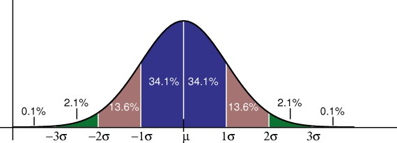
The statistical parameter used to quantify the width of the Gaussian bell curve is the standard deviation, known as sigma, also often referred in the GIS world to as the root-mean-square-error (RMSE). Given a large enough sample of measurements, 68% will fall within one sigma of the mean, 95% will fall within about two sigma (1.96*sigma, to be precise), and 99.8% will fall within three sigma. When comparing a spatial dataset to a sample of ground checkpoints, one can plot the differences between the observed coordinates and the checkpoint coordinates, compute the mean error and RMSE using standard statistical formulas, and report accuracy at the 95% confidence limit as a function of RMSE.
Remember that the basic assumption one makes when applying the normal distribution as an appropriate error model is that there are no irregularities or artifacts in the data that would cause the actual error distribution to differ from the ideal Gaussian bell curve. Furthermore, for RMSE to apply as a statement of absolute positional accuracy, there can be no biases or systematic errors in the dataset that cause the average error to be significantly non-zero. Remotely sensed datasets may contain systematic errors, either due to characteristics of the sensor or characteristics of the target. In the lesson material to come, you will see examples of this, and you will see how the statistics used in accuracy assessment help to point out these biases and diagnose their cause.
Validation of Orthorectified Imagery
One of the first points to make in a discussion about spatial accuracy of orthorectified imagery is that accuracy is completely unrelated to spatial resolution. The size of a pixel has no physical bearing on the accuracy of its location in the ground coordinate system. Spatial accuracy depends only on the quality of the georeferencing, either as applied from ground control with aerotriangulation or provided by direct georeferencing. The difference between spatial accuracy and spatial resolution is often overlooked or unrecognized by the layman, and it is often not made clear to the uninitiated public consumer in marketing literature or by the news media.
The size of an object that can be seen in an image, compared to the accuracy of its location as derived from the image, may be significantly different. For example, the standard USGS and NAIP DOQQ products were produced at a 1-meter GSD with a targeted horizontal accuracy of about 10 meters at the 90% confidence level compared to ground surveyed checkpoints. When circumstances and budgets permit, it is desirable to specify a spatial accuracy requirement that is comparable to the size of a pixel in ground units. For example, if the output image pixel size is 1 meter, then the spatial accuracy requirement might be defined such that each 1-meter pixel in the image was assured to be within 2 meters of its "true" location in the ground coordinate system at the 95% confidence limit. The general rule of thumb is to target a root-mean-square-error (RMSE) for spatial accuracy equivalent to the size of a pixel (GSD) in the output image. In practice, and depending on the end user application, it is not always possible or necessary to follow this rule. If the primary purpose of the imagery is simply to identify objects and measure their size relative to each other, then the absolute spatial accuracy in terms of ground coordinates may be less important than relative accuracy or spatial resolution. If the objective is to create secondary map products from the orthorectified imagery, such as building footprints or road centerlines, then the absolute accuracy should be comparable to resolution.
In the interest of economy, some image data products are generated using control extracted from other image sources, rather than using new ground control or direct georeferencing data acquired along with the new imagery. This is akin to the exercise we performed in the final part of the Lesson 3 lab, using image points I provided as a source of control for orthorectification. Many USDA NAIP DOQQs use USGS DOQQs as a source of georeferencing control. Furthermore, they often use the USGS DOQQs as a source of "independent" check points; so that the accuracy that is reported is a comparison to the USGS image, not the actual ground. The following quote, consistent with USDA NAIP program specifications, is extracted from the metadata of the 2005 NAIP DOQQs for the state of Minnesota [47], "the source quarter-quad files are 2 meter ground sample distance (GSD) orthoimagery rectified to a horizontal accuracy of within 10 meters of reference digital orthophoto quarter quads (DOQQ's) from the National Digital Ortho Program (NDOP)." This is a statement of relative accuracy, not of absolute accuracy. One must read the metadata carefully to understand the distinction; relying on software, simply reading the RMSE from a metadata field, may lead to faulty assumptions about the spatial accuracy of the data one is using for analysis.
Data Validation
Acceptance of an orthorectified image deliverable should validate all the product specifications defined by the end user. There are three general categories of quality control and quality assurance checks and tests:
- Data Integrity - do the files contain what they are supposed to contain?
- Spatial Accuracy - do the data products meet the end user requirements for horizontal accuracy?
- Aesthetics - do the data products meet the customer's expectations in terms of color balancing, edge matching from photo to photo, and other general image quality characteristics?
Simply viewing the imagery in a GIS environment accomplishes the data integrity step. This cursory view can ensure that:
- individual image files are in the correct format and the files have not been corrupted;
- complete coverage of the area of interest has been achieved;
- accurate georeferencing information exists for each image file, in the specified coordinate system;
- size of image pixels matches the data product specification.
Quantitative Assessment
Orthorectified imagery is very often used as a visual backdrop to other GIS data or as a source for image interpretation and collection of point, line, or polygon features to be used in GIS. Because of this widespread use as a base map, quantitative accuracy assessment is one of the most important aspects of orthophoto quality assurance and acceptance testing.
An orthophoto is essentially a 2-dimensional product. As we learned in Lesson 3, the fidelity and accuracy of the terrain model used in the rectification process has an impact on the horizontal accuracy of the orthophoto; however, the image dataset has no elevation information contained explicitly within it. Horizontal accuracy is the only relevant spatial accuracy assessment metric. The end user's accuracy specification is commonly stated as a root-mean-square-error (RMSE) based on measurements of well-defined points in the imagery compared to independent survey measurements of higher accuracy serving as ground truth. The definition of a well-defined point, guidance on the selection and surveying of these checkpoints, and the methodology for calculating the RMSE is documented in the National Standard for Spatial Data Accuracy [48] (NSSDA) published by the US Federal Geographic Data Committee.
For historical reasons, mapping accuracies are commonly specified at the 95% confidence limit. A typical accuracy statement accompanying an orthophoto deliverable would be "Tested ____ (meters, feet) horizontal accuracy at 95% confidence level," and the numerical value supplied is RMSE * 1.7308. This statement of accuracy assumes that no systematic errors or biases are present in the data and that the individual checkpoint errors follow a normal distribution, independent in the x and y directions. Note that the multiplier for the RMSE is 1.7308, rather than the 1.96 factor stated in the Introduction page of this lesson. Horizontal error is a circular error, a combination of the independent linear errors in the x and y dimensions.
Most professional practitioners involved in the design of a remote sensing data acquisition know how to design a project to meet the designated accuracy specification. When errors exceed specification, there is usually a systematic cause. Common problems are instrument misalignment or miscalibration, georeferencing system drifts, and blunders in datum or coordinate system conversion. Systematic errors such as these can be detected by examining other statistical metrics and plotting the spatial distribution of the errors. In a dataset containing systematic errors, the mean of the errors will be non-zero and the entire may be shifted north, south, east, or west from its proper location. Systematic trends are easily detectable and can usually be related to a physical cause. Once the cause has been determined, systematic errors can often be corrected by reprocessing the data. Only when systematic errors have been successfully removed does the RMSE or 95% confidence statement give the user a true indication of the absolute accuracy of the data product.
The process of accuracy assessment begins with collection of a number of ground checkpoints, usually surveyed with GPS, accompanied by a set of field sketches and photographs to aid the image analyst in proper identification in the orthophoto image. Figure 2 shows an example of such a check point, chosen because it can be clearly and unambiguously identified in the orthophoto to be tested.
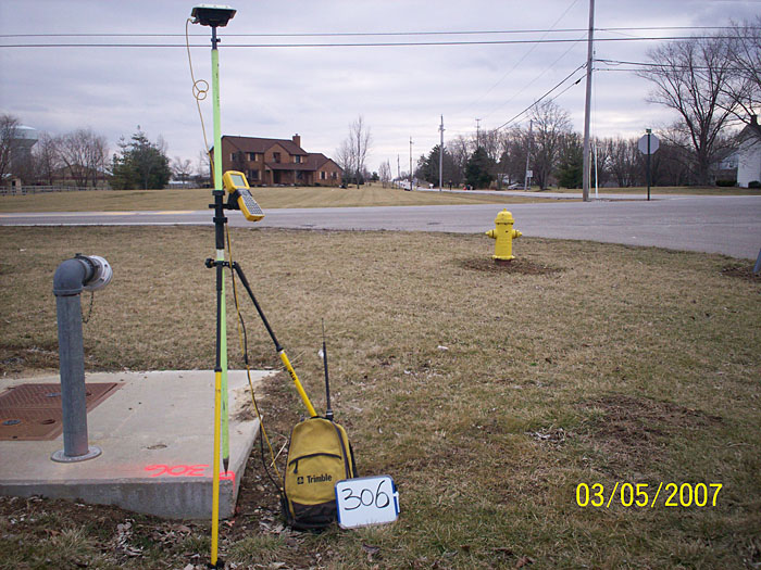
The survey sketch shown in Figure 3 above is an important complement to the digital photograph. The sketch provides additional information about the vicinity of the point that helps the image analyst navigate to the correct vicinity of the point. Armed with the surveyed coordinate derived GPS, the digital photo, and the field sketch, the image analyst should be able to locate the point within the project area, identify the correct orthophoto image within the project database to be examined, and navigate to the exact location of the point, as shown in Figure 4. The surveyed coordinates, derived from GPS, are then compared to the coordinate readout from the orthophoto in GIS or CAD software.
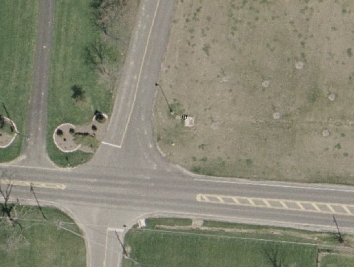
The image analyst visits and records the coordinates for each surveyed checkpoint in the orthophoto imagery. This can be done quite easily in GIS software. The survey results can be imported as a point file and overlaid on the orthophoto with identifying labels. The points should fall very close to the correct location, and the image analyst has only to confirm the exact location, using the photo and the sketch. The image point measurements are recorded in another point file. A table of coordinates can be exported from the GIS or CAD software and used to generate graphs and statistics, such as mean error in each direction, RMSE and 95% confidence values.
Qualitative Assessment
The final step of acceptance testing involves an examination of general image quality. The imagery for a large project may have been flown over a period of weeks under varying lighting conditions. Matching and balancing the brightness, contrast, and color tones may require use of image processing software.
The USDA developed a set of documents describing the type of visual artifacts they commonly see in orthophoto deliverables to the NAIP program. Because this type of visual inspection goes beyond the intended scope of this lesson, it won't be discussed in the lesson material. Feel free to review the referenced documents, which have been made available through the course download site. These are specific to a particular federal imagery program; however, the types of artifacts encountered and the image processing techniques recommended to overcome them can be widely applied.
- FSA User Sensitivity Study for Quality of National Agricultural Imagery Program (NAIP) Imagery [50] - Interim Technical Report looks at end user sensitivity to aesthetic issues, such as noise, sharpness, color registration, color saturation, color balance, and tonal variation. The report is a valuable example because it examines the impact of these issues in the context of the intended application. While aesthetic defects may be distracting or annoying from a purely aesthetic point of view, the prescribed remedy may not produce sufficient benefits to justify the cost or time required to implement.
- Aerial Photography Field Office-National Agriculture Imagery Program (NAIP) Suggested Best Practices [51] - Final Report provides guidelines and recommendations for the use of image processing techniques to effectively remedy defects identified in the User Sensitivity Study.
- Aerial Photography Field Office-Scaled Variations Artifact Book [52] provides a number of graphic examples of the defects before and after image processing remedies have been applied.
Validation of Elevation Data
The approach and methods for vertical accuracy testing of terrain data are very similar to those presented above for orthorectified imagery. Elevations are measured relative to a vertical datum, and the vertical datum itself is an approximation of something ideal such as “mean sea level,” which cannot be exactly and completely known, because it is by definition an average. We cannot say absolutely that a particular elevation is accurate to within 1 foot, 1 inch, or 1 millimeter of its true value. However, we can express the level of confidence we have in a measurement based on a framework of statistical testing. Based on a sample of independent elevation check points, we can say we have a level of confidence that any other point in the entire dataset is within the stated tolerance of its “true” value expressed relative to one vertical datum or another.
In this course, you have been introduced to the distinctly different technologies for capturing terrain data that have come into maturity in recent decades: photogrammetry, lidar, and IFSAR. Because these technologies are so new to both data providers and end users, the topic of QA/QC of terrain data has been the subject of much debate and study. Not only is there a high level of interest in applications that make use of terrain data, there is also a pervasive need to understand the strengths and weaknesses of each technology in order to make good investment decisions in equipment, software, and data.
As discussed above, the QA/QC process gives us insight into the types of errors and artifacts that affect terrain data, due either to the sensor or to characteristics of the target surface. With respect to the terrain data, there was concern from the start that vertical accuracy would vary within a single dataset, based on the type of terrain and land cover being mapped. In other words, there was some recognition that accuracy itself was a spatial variable. While this is undoubtedly true of most spatial datasets, including orthorectified imagery, the discussion and debate about methods of accuracy assessment and reporting have been highly focused on terrain, and it’s safe to say that there will be significant refinements and developments occurring in the next decade.
In the final content section of this lesson, you will see that the current standards for elevation data accuracy assessment and reporting are actually called guidelines, and that there are a number of unanswered questions on the table that require further research. Overall, this represents progress, because there is widespread recognition that the quantification of error within a dataset is more complex than a simple calculation of RMSE.
Data Validation
Quality control and assurance for terrain models comprise the three categories, similar to those introduced previously for orthorectified imagery:
- Data integrity, which includes completeness of coverage at the user-defined post-spacing or density, valid files in the user-defined format, and accurate georeferencing information.
- Spatial accuracy, which for terrain models is primarily vertical accuracy; however, for some products such as breaklines, horizontal accuracy is also relevant.
- Visual inspection for artifacts and anomalies, which for terrain data, is not only aesthetic, but affects accuracy of the terrain surface.
Terrain data come in many different forms (DEM, DTM, DSM, TIN, breaklines, etc.) and formats. It is important to ensure that the user has specified this clearly before production begins, as transforming from one format to another after production is time-consuming and may introduce undesirable interpolation errors into the data itself. It is best to provide users with a small sample area as soon as possible, before beginning full production, to allow them the chance to use the sample data on their own systems and with their own software.
Quantitative Assessment
As with horizontal data and checkpoint, the reference elevation data ought to be at least three times more accurate than the sample data. The root-mean-square error (RMSE) as calculated between the sample dataset and the independent source is converted into a statement of vertical accuracy at an established confidence level, normally 95 percent. Because elevation is a one-dimensional variable, the 95% confidence level is equivalent to the RMSE multiplied by 1.96. A NSSDA-compliant accuracy statement accompanying a terrain model deliverable would be “Tested ____ (meters, feet) vertical accuracy at 95% confidence level”, and the numerical value supplied is RMSE * 1.9600. This statement of accuracy assumes that no systematic errors or biases are present in the data and that the individual checkpoint errors follow a normal distribution.
One of the biggest potential customers for terrain data in the United States is FEMA, in particular the national floodplain mapping program. As topographic lidar was emerging as a powerful terrain mapping tool in the mid to late 1990s, one of FEMA’s most pressing questions was “how does it perform in the different land cover types that characterize the floodplain?” This question and FEMA’s potential need for accurate elevation data nationwide drove the development of guidelines and specifications for lidar acquisition, processing, QA/QC, and accuracy testing. The FEMA guidelines required testing and reporting against independent check points in representative land cover types. The most common land cover types identified for terrain model accuracy assessment purposes are: open ground, weeds and crops, scrub and shrub, forest and urban.
The FEMA guidelines are presented in more depth later in the lesson; for the moment, it is relevant to point out that the early testing of lidar data, according to these guidelines, pointed out several important facts that affect our approach to quantitative accuracy assessment of terrain data. First and foremost, it was discovered that errors in lidar-derived terrain datasets do not follow a normal distribution, except over bare ground. In areas covered by any sort of vegetation, the tendency will be for lidar (and for radar as well) to yield elevations above the ground due to returns off the canopy. In built-up areas, there will be many lidar returns on objects above the ground, which may not all be removed from the bare earth terrain model, again causing an asymmetric error distribution with more above-ground errors than below-ground errors. On the contrary, lidar tends to measure elevations a bit below the ground on the dark asphalt surfaces that are common to roadways and urban areas. When one begins to study the error distribution for an entire dataset in detail, it is obvious that accuracy not only varies within the dataset due to variation in land cover, but it also deviates from a normal error distribution in particular ways depending on the slope, roughness, and composition of the surface. One can easily assume that radar will have its own set of similar issues.
In recognition of the fact that errors in lidar-derived terrain models are often not appropriately modeled by a Gaussian distribution, a nonparametric testing method, based on the 95th percentile, was proposed and implemented in the National Digital Elevation Program Guidelines. According to these guidelines (which are the currently-accepted working standard for most lidar projects in the US, including those conducted for FEMA), fundamental vertical accuracy is measured in bare, open terrain and reported at the 95% confidence level as a function of vertical RMSE; in other land cover types, the supplemental or consolidated vertical accuracy is measured and reported according to the 95th percentile method. Both Maune (2007) and the NDEP Guidelines give detailed instructions for the computation of these quantities. Links to those documents are provided on page 8 of this lesson.
A sample vertical accuracy assessment report [53], compiled by an independent contractor for the Pennsylvania statewide lidar program, PAMAP, illustrates the calculation and reporting of quantitative accuracy assessment results.
Qualitative Assessment
The final step in product acceptance is the qualitative assessment. Various 3D visualization techniques are used to view the terrain surface and examine it for artifacts, stray vegetation or buildings and the like. Water bodies tend to pose special problems and generally require some sort of manual editing during data production, so lakes, rivers, and shorelines should be examined to ensure that as an elevation surface, they are represented as being flat. The elevation used over water bodies is almost never an accurate representation of the height of the water surface in reality, because most remote sensing techniques do not directly measure water heights reliably. In a terrain model product, the elevation of a water body is usually filled in using the mean elevation of the shoreline.
Breaklines are normally a supplemental deliverable accompanying another type of terrain model (DEM, DTM, or DSM). The most common way to assess the quality and accuracy of breaklines is superimposition on the terrain model in a 3-dimensional view. Contours are usually generated from another type of terrain model, so they are usually not checked directly for vertical accuracy. They should be checked to ensure that they do not cross, touch or contain gaps.
A sample QA/QC report [54], compiled by an independent contractor for the Pennsylvania statewide lidar program, PAMAP, provides many good examples of the types of artifacts found in visual inspection of a lidar-derived terrain dataset. It is difficult to automate identification and correction of these artifacts; therefore, the independent review and final data editing is usually an interactive process involving the data producer, the independent reviewer, and the data purchaser.
Lesson 7: Basic Concepts of Image Analysis
Lesson 7 Introduction
Image analysis is a broad term encompassing a wide variety of human and computer-based methods used to extract useful information from images. Three major categories of image analysis are relevant to this discussion. Image interpretation is performed by a human, using technology to facilitate speedy viewing and recording of observations. Digital image classification techniques are used to delineate areas within an image based on a classification scheme relevant to the application. Change detection applies to two or more images acquired over the same location; change detection results may also be classified in terms of the type of change and quantified in terms of the amount or degree of change.
Lesson 1 introduced the physical basis for spectral analysis of remotely sensed imagery. We departed from that fundamental background into topics central to mapping and map products. In Lesson 7, we will return to the fundamental physical concepts in a deeper look at state-of-the-art sensors, platforms, and methods for extracting information content from multispectral data.
Until very recently, spaceborne sensors produced the majority of multispectral data. Federal agencies distribute some of their data at no cost. Commercial data providers (SPOT, GeoEYE, Digital Globe, and others) license imagery to end-users for a fee, with limits on further distribution. Airborne multispectral data, from sensors such as the Leica ADS-40, the Intergraph DMC, and the Vexcel UltraCam, is becoming available in the public domain through the US Department of Agriculture (USDA) National Agriculture Imagery Program (NAIP).
Multispectral satellite imagery is often georeferenced but not orthorectified; further processing is required to be able to overlay the data in GIS with other vector layers. The imagery you will be using in the Lesson 7 activity has already been rigorously orthorectified, but if it were not, you have been given the tools and skills to be able to do that yourself, using ArcMap and Geomatica.
Lesson Objectives
At the end of this lesson, you will be able to:
- describe and perform image enhancement techniques to improve interpretability of imagery;
- describe common image interpretation tasks;
- describe eight elements of image interpretation;
- perform simple supervised and unsupervised classification using automated methods.
Questions?
If you have any questions now or at any point during this week, please feel free to post them to the Lesson 7 Questions and Comments Discussion Forum in Canvas.
Multispectral Remote Sensing Systems
The origins of commercial multispectral remote sensing can be traced to interpretation of natural color and color infrared (CIR) aerial photography in the early 20th century. CIR film was developed during World War II as an aid in camouflage detection (Jensen, 2007). It also proved to be of significant value in locating and monitoring the condition of vegetation. Healthy green vegetation shows up in shades of red; deep, clear water appears dark or almost black; concrete and gravel appear in shades of grey. CIR photography captured under the USGS National Aerial Photography Program [14] was manually interpreted to produce National Wetlands Inventory (NWI) maps for much of the United States. While film is quickly being replaced by direct digital acquisition, most digital aerial cameras today are designed to replicate these familiar natural color or color-infrared multispectral images.
Computer monitors are designed to simultaneously display 3 color bands. Natural color image data is comprised of red, green, and blue bands. Color infrared data is comprised of infrared, red, and green bands. For multispectral data containing more than 3 spectral bands, the user must choose a subset of 3 bands to display at any given time, and furthermore must map those 3 bands to the computer display in such as way as to render an interpretable image. Module 2 of the Esri Virtual campus course, “Working with Rasters in ArcGIS Desktop,” gives a good overview of the display of multiband rasters and common 3-band combinations of multiband data sets from sensors such as Landsat and SPOT.
Spaceborne Sensors
Since the 1967 inception of the Earth Resource Technology Satellite (ERTS) program (later renamed Landsat), mid-resolution spaceborne sensors have provided the vast majority of multispectral datasets to image analysts studying land use/land cover change, vegetation and agricultural production trends and cycles, water and environmental quality, soils, geology, and other earth resource and science problems. Landsat has been one of the most important sources of mid-resolution multispectral data globally. The history of the program and specifications for each of the Landsat missions is covered in Chapter 6 of Campbell (2011).
The French SPOT satellites have been another important source of high-quality, mid-resolution multispectral data. The imagery is sold commercially, and is significantly more expensive than Landsat. SPOT can also collect stereo pairs; images in the pair are captured on successive days by the same satellite viewing off-nadir. Collection of stereo pairs requires special control of the satellite; therefore, the availability of stereo imagery is limited. Both traditional photogrammetric terrain extraction techniques, as well as automatic correlation, can be used to create topographic data in inaccessible areas of the world, especially where a digital surface model may be an acceptable alternative to a bare-earth elevation model.
Digital Globe (QuickBird and WorldView) and GeoEye (IKONOS and OrbView) collect high-resolution multispectral imagery which is sold commercially to users throughout the world. US Department of Defense users and partners have access to these datasets through commercial procurement contracts; therefore, these satellites are quickly becoming a critical source of multispectral imagery for the geospatial intelligence community. Bear in mind that the trade-off for high spatial resolution is limited geographic coverage. For vast areas, it is difficult to obtain seamless, cloud-free, high-resolution multispectral imagery within the single season or at the particular moment of the phenological cycle of interest to the researcher.
Airborne Sensors
Digital aerial cameras were developed to replicate and improve upon the capabilities of film cameras; therefore, most commercially available medium and large-format mapping cameras produce panchromatic, natural color, and color-infrared imagery. They are, in fact, multispectral remote sensing systems. Most are based on two-dimensional area arrays. The Leica Geosystems ADS-40, which makes use of linear array technology, is the exception. This sensor was described in some detail in Lesson 2. The unique design of this instrument allows it to capture stereoscopic imagery in a single pass, but georeferencing of the linear array data is more complex than for a frame image.
The ADS-40 and the Z/I Digital Modular Camera (DMC) are being used extensively in the USDA NAIP program to capture high-resolution multispectral data over most of the conterminous United States each growing season. Be aware, however, that NAIP data, other than the fact that it is orthorectified to National Digital Orthophoto Program (NDOP) standards, is not extensively processed or radiometrically calibrated. The USDA uses it primarily for visual verification and interpretation, not for digital classification.
Georeferencing
Georeferencing an analog or digital photograph is dependent on the interior geometry of the sensor as well as the spatial relationship between the sensor platform and the ground. The single vertical aerial photograph is the simplest case; we can use the internal camera model and six parameters of exterior orientation (X, Y, Z, roll, pitch, and yaw) to extrapolate a ground coordinate for each identifiable point in the image. We can either compute the exterior orientation parameters from a minimum of 3 ground control points using space resection equations, or we can use direct measurements of the exterior orientation parameters obtained from GPS and IMU.
The internal geometry of design of a spaceborne multispectral sensor is quite different from an aerial camera. The figure below (from Jensen, 2007, Remote Sensing of the Environment) shows six types of remote sensing systems, comparing and contrasting those using scanning mirrors, linear pushbroom arrays, linear whiskbroom areas, and frame area arrays. The digital frame area array is analogous to the single vertical aerial photograph.
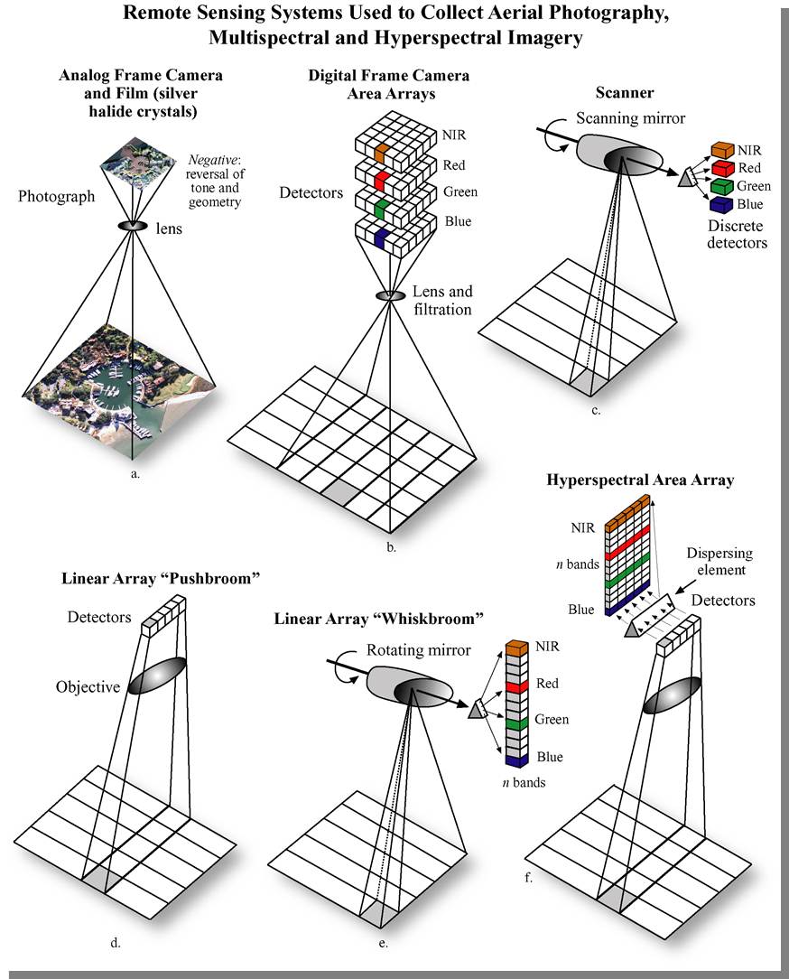
A linear array, or pushbroom scanner, is used in many spaceborne imaging systems, including SPOT, IRS, QuickBird, OrbView, and IKONOS. The position and orientation of the sensor are precisely tracked and recorded in the platform ephemeris. However, other geometric distortions, such as skew caused by the rotation of the earth, must be corrected before the imagery can be referenced to a ground coordinate system.
Several airborne systems, the Leica ADS-40 and the ITRES CASI, SASI, and TABI, also employ the pushbroom design. Each line of imagery is captured at a unique moment in time, corresponding with an instantaneous position and attitude of the aircraft. When direct georeferencing is integrated with these sensors, each single line of imagery has the exterior orientation parameters needed for rectification. However, without direct georeferencing, it is impossible to reconstruct the image geometry; the principles of space resection only apply to a rigid two-dimensional image.
The internal geometry of images captured by spaceborne scanning systems is much more complex. Across-track scanning and whiskbroom systems are more akin to a lidar scanner than to a digital area array imager. Each pixel is captured at a unique moment in time; the instantaneous position of the scanning device must also be factored into the image rectification. For this reason, a unique (and often proprietary) sensor model must be applied to construct a coherent two-dimensional image from millions of individual pixels. Add to this complexity the fact that there is actually a stack of recording elements, one for each spectral band, and that all must be precisely co-registered pixel-for-pixel to create a useful multiband image.
Direct georeferencing solves a large part of the image rectification problem, but not all of it. Remember, in our discussions of space resection and intersection, we learned that we can only extrapolate an accurate coordinate on the ground when we actually know where the ground is in relationship to the sensor and platform. We need some way to control the scale of the image. Either we need stereo pairs to generate intersecting light rays, or we need some known points on the ground. A georeferenced satellite image can be orthorectified if an appropriate elevation model is available. The effects of relief displacement are often less pronounced in satellite imagery than in aerial photography, due to the great distance between the sensor and the ground. It is not uncommon for scientists and image analysts to make use of satellite imagery that has been registered or rectified, but not orthorectified. If one is attempting to identify objects or detect change, the additional effort and expense of orthorectification may not be necessary. If precise distance or area measurements are to be made, or if the analysis results are to be used in further GIS analysis, then orthorectification may be important. It is important for the analyst to be aware of the effects of each form of georeferencing on the spatial accuracy of his/her analysis results and the implications of this spatial accuracy in the decision-making process.
Preprocessing
Defining characteristics of remote sensing instruments, platforms, and data were discussed in Lessons 1 and 2. Any remotely-sensed image or dataset can be defined in these terms and evaluated against the end-user application requirements to determine potential suitability. A raw scene can be produced in real-time or near-real-time from most digital sensors, and can be distributed as fast as the technology infrastructure allows. Simple visual interpretation can be quite useful for general situational awareness and decision-making. Most of us saw daily satellite images over the New Orleans Superdome after Hurricane Katrina and can appreciate the positive impact of these lightly-processed datasets.
Additional preparation and processing is often required for any more complex analysis. If the end-user application requires the overlay of multiple remotely sensed images or detailed GIS data, such as road centerlines and property boundaries, georeferencing must be performed. If spectral information is to be used to classify pixels or areas in the image based on their content, then the effects of the atmosphere must be accounted for. To detect change between multiple images, both georeferencing and atmospheric correction of all individual images may be required.
Georeferencing: The degree of accuracy and rigor required for the georeferencing depends on the desired accuracy of the result. More error can be tolerated in an image backdrop intended for visual interpretation, where a human interpreter can use judgment to work around some geographic misalignments. If the intent is to use automated processing to intersect, combine, or subtract one data layer from the other using mathematical algorithms, then the spatial overlay must be much more accurate in order to produce meaningful results. Higher accuracy is achieved only with better ground control, accurate elevation data, and thorough quality assurance. Most remotely-sensed data is delivered with some level of georeferencing information, which locates the image in a ground coordinate system. There are generally three levels of georeferencing, each corresponding to a different geometric accuracy.
- Level 1: uses positioning information obtained directly from the sensor and platform to roughly geolocate the remotely-sensed scene on the ground. This level of georeferencing is sufficient to provide geographic context and support visual interpretation of the data. It is not often not accurate enough to support robust image or GIS analysis that requires combining the remotely-sensed dataset with other layers.
- Level 2: uses a Digital Elevation Model (DEM) to remove relief displacement caused by variation in the height of the terrain. This improves the relative spatial accuracy of the data; distances measured between points within the geo-corrected image will be more accurate, particularly in scenes containing significant elevation changes. The DEM is usually obtained from another source, and the spatial accuracy of the Level 2 image will depend on the accuracy of the DEM.
- Level 3: uses a DEM and ground control points to most accurately georeferenced the image on the ground. In addition to the DEM, ground control points must be obtained from another source, and the accuracy of the Level 3 image will depend on the accuracy of the ground control points. Level 3 processing is usually required in order to provide the most accurate overlays of remotely-sensed data sets and other relevant GIS data.
Most satellite imagery is distributed with Level 1 georeferencing, which is often sufficient for making quick visual assessments of conditions on the ground. Additional processing to Level 2 or 3 (involving additional time and expense) is usually needed to analytically compare multiple scenes over the same location or precisely overlay other types of geographic information, such as property boundaries or building footprints. End-users may choose to perform this additional processing themselves, if they have the requisite control materials, expertise, and time.
Atmospheric Correction: If the end-user application intends to make use of spectral information contained in the image pixels to identify and separate different types of material or surfaces based on sample spectral libraries, then contributions to those pixels values made by the atmosphere must be removed. Atmospheric correction is a complex process utilizing control measurements, information about the atmospheric content, and assumptions about the uniformity of the atmosphere across the project area. The process is automated, but requires sophisticated software, highly skilled technicians, and again, time. Furthermore, atmospheric correction parameters used on one dataset cannot be summarily applied to a dataset collected on another day.
Image Interpretation
From a technology perspective, the simplest way to extract information from remotely sensed data is human interpretation. However, significant training and experience are needed to produce a skilled image interpreter. (Campbell, 2007) Eight elements of image interpretation employed by human image interpreters are:
- Image tone: the lightness or darkness of a region within an image.
- Image texture: the apparent roughness or smoothness of a region within an image.
- Shadow: may reveal information about the size and shape of an object which cannot be discerned from an overhead view alone.
- Pattern: the arrangement of individual objects in distinctive recurring patterns, such as buildings in an industrial complex or fruit trees in an orchard.
- Association: the occurrence of one type of object may infer the presence of another commonly associated object nearby.
- Shape: man made and natural features often have shapes so distinctive that this characteristic alone provides clear identification.
- Size: the relative size of an object related to other familiar objects gives the interpreter a sense of scale, which can aid in the recognition of objects less easily recognized.
- Site: refers to topographic position. For example, certain crops are commonly grown on hillsides or near large water bodies.
Tasks common to image interpretation are:
- Classification: assigning objects, features, or areas to classes. This occurs at three levels of confidence.
- Detection: determining the presence or absence of a feature.
- Recognition: assigning an object or feature to a general class or category.
- Identification: specifying the identity of an object with enough confidence to assign it to a very specific class.
- Enumeration: listing or counting discrete items visible on an image.
- Mensuration: measurement of objects and features in terms of distance, height, volume, or area.
- Delineation: drawing boundaries around distinct regions of the image characterized by specific tones or textures.
The results of image interpretation are most often delivered as a set of attributed points, lines, and/or polygons in any one of a variety of CAD or GIS data formats. The classification scheme or interpretation criteria must be agreed upon with the end user before the analysis begins.
Band Assignment
The interpretability of multispectral images can be improved through the spectral enhancement of the image. Such enhancements can either be temporary and reversible, or they can result in the creation of new data layers. Image enhancements that are commonly used to support the analysis of remotely sensed imagery.
Color Assignment for Computer Displays
By now, you should be familiar with the characteristics of the natural color image, the image which most closely resembles what you would expect to see looking down at earth from a plane. To create a natural color image, the spectral bands from the image are matched directly to the representative color display channels, or color guns, of the computer. For example, the red spectral band of a Landsat Image is matched to the Red color display channel on the computer, while the Green spectral band is matched to the Green color display and so on. In Figure 1.a, the natural colors of the scene provide adequate contrast between the urban areas and the forest; however, when compared to the other images in this figure, you will notice additional features that are not readily apparent in this natural color image. The reassignment of spectral bands to different color guns can improve the visibility of some image feature.
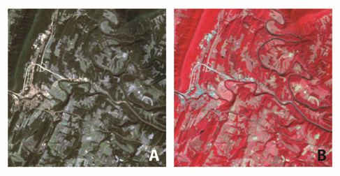
False-color-composite images are frequently used in remote sensing. The false-color-composite image is created by assigning spectral bands to color guns in combinations that do not create a natural color image. A common false-color-composite image used to support analysis of vegetation reassigns the near-infrared spectral band to the red color gun, the red spectral band to the green color gun, and the green spectral band to the blue color gun. The image that results from this combination is very different than the natural color image that you are used to seeing, as shown in Figure 1.b.
The major benefit of the false-color-composite is the increased ability to detect variations in vegetation due to the fact that vegetation strongly reflects NIR energy. In Figure 1.b, notice that it becomes easier to identify water features from the forested areas. In the natural color image, the lake in the lower left-hand corner blends in with the surrounding forest cover; the false-color-composite image highlights the lake's location. Fallow fields are evidenced by bright blue and white colors, while fields where crops have already grown are shown in the light pink angular patches that scatter across the darker red forests.
Band Math
The image enhancements that use the computer display to alter the appearance of an image are impermanent; they are usually saved only in the software project document. It is also possible to use mathematical and statistical methods to exploit relationships between spectral bands to create new archivable raster data products that can be also be interpreted. The Normalized Vegetation Difference Index (NDVI) is an example of such a product that is commonly used to support analysis of vegetation.
The calculation of NDVI is very straightforward. It is the ratio of the subtraction of the near-infrared and red bands to their sum [(NIR-RED)/(NIR+RED)], and its value ranges from -1 to 1, where green vegetation typically ranges between 0.2 and 0.9. In Figure 2, the NDVI image is useful for identifying agricultural fields that are in different phases of growth. Fallow fields here are dark, having low NDVI values, while green vegetation, such as the forests on the ridgeline, are much brighter. The NDVI image emphasizes the location of water bodies and impervious surfaces (black), but does a poor job of differentiating between the two based on value alone. Instead, the visual interpretation element of shape can be used to differentiate here the meandering river and the relatively straight roadway.
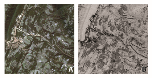
More sophisticated methods of analyzing spectral data also exist. The Tasseled-Cap Transformation is a statistical method for reducing multispectral data. First designed to support agricultural analysis (Kauth and Thomas 1976), it has also been shown to be useful in land cover change mapping (Healey et al. 2005). Like NDVI described above, this transformation takes advantage of the differences in NIR and RED reflectance.
The Tasseled-Cap Transformation decomposes a multispectral image into three main components that comprise 97% of the Landsat spectral data content; these components are brightness, greenness, and wetness. Each is said to be related to particular physical feature types:
- Brightness, Figure 2B, is assigned to the Red color display channel is associated with impervious surfaces such as asphalt.
- Greenness, Figure 2C, is assigned to the Green color display, is associated with vegetation.
- Wetness, Figure 2D, is assigned to the Blue color display, is associated with moisture.
Each of the three components can be visualized separately; however, when combined, these three components can provide great insights into the landscape as shown in Figure 2A. This Tasseled-Cap Color image highlights differences between features that are not found by looking at the NDVI image. For example, it is possible to identify a road feature by its thin linear shape and low reflectance values in the NDVI image. Looking at that same feature, Tasseled-Cap Color image, reveals more subtle differences. Look at the small built-up area in the left of the images. In the NDVI image, this feature looks to be one feature, however, looking at the Tasseled-Cap image we can see that what seemed to be a single feature really is many smaller features.
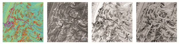
You have now looked at several methods for enhancing the spectral data from remotely sensed images. In order to maximize the usefulness of such transformations, an analyst must choose the enhancement most appropriate to the task at hand. Spectral enhancements alone are not enough on their own to make interpretation accurate; a good command of the various interpretation elements, combined with strong contextual knowledge of the image under analysis, contributes to successful interpretation.
Healey, S. P., W. B. Cohen, Y. Zhiqiang & O. N. Krankina (2005) Comparison of Tasseled Cap-based Landsat data structures for use in forest disturbance detection. Remote Sensing of Environment, 97, 301-310.
Kauth, R. J. & G. Thomas. 1976. The tasseled cap--a graphic description of the spectral-temporal development of agricultural crops as seen by Landsat. In LARS Symposia, 159.
Digital Image Classification
Digital image classification uses the quantitative spectral information contained in an image, which is related to the composition or condition of the target surface. Image analysis can be performed on multispectral as well as hyperspectral imagery. It requires an understanding of the way materials and objects of interest on the earth's surface absorb, reflect, and emit radiation in the visible, near-infrared, and thermal portions of the electromagnetic spectrum. In order to make use of image analysis results in a GIS environment, the source image should be orthorectified so that the final image analysis product, whatever its format, can be overlaid with other imagery, terrain data, and other geographic data layers. Classification results are initially in raster format, but they may be generalized to polygons with further processing. There are several core principles of image analysis that pertain specifically to the extraction of information and features from remotely sensed data.
- Spectral differentiation is based on the principle that objects of different composition or condition appear as different colors in a multispectral or hyperspectral image. For example, a newly planted cornfield has a distinct color when compared to a field of mature plants, and yet another color when the field has been harvested. Corn has a distinct color as compared to wheat; healthy plants are a different color than pest-infested or drought-impacted plants. The use of spectral signature, or color, to distinguish types of ground cover or objects is called spectral differentiation.
- Radiometric differentiation is the detection of differences in brightness, which may in certain cases be used to inform the image analyst as to the nature or condition of the remotely sensed object.
- Spatial differentiation is related to the concept of spatial resolution. We may be able to analyze the spectral content of a particular pixel or group of pixels in a digital image when those pixels comprise a single homogeneous material or object. It is also important to understand the potential for mixing of the spectral signatures of multiple objects into the recorded spectral values for a single pixel. When designing an image analysis task, it is important to consider the size of the objects to be discovered or studied compared to the ground sample distance of the sensor.
The extraction of information from remotely sensed data is frequently accomplished using statistical pattern recognition; land-use/land-cover classification is one of the most frequently used analysis methods (Jensen, 2005). Land cover refers to the physical material present on the earth’s surface; land use refers to the type of development and activities people undertake in a particular location. The designation of “woodland” for a tree-covered area is a land cover classification; the same woodland might be designated as “recreation area” in a land use classification.
While certain aspects of digital image classification are completely automated, a human image analyst must provide significant input. There are two basic approaches to classification, supervised and unsupervised, and the type and amount of human interaction differs depending on the approach chosen.
- Supervised classification requires the image analyst to choose an appropriate classification scheme, and then identifies training sites in the imagery that best represent each class. A simple land cover classification scheme might consist of a small number of classes, such as urban, water, wetlands, forest, grass/crops. Individual sites that fall into a single class may have slightly different spectral characteristics; for example, the spectral signature of a water body will depend on the amount of suspended sediment or plant material in the water. Urban land cover signatures will vary based on the type of materials used; asphalt has a very different spectral signature from concrete, wood, or glass. The image analyst must select a sufficient number of training sites in each class to represent the variation present within each class in the image. The classification algorithm then uses spectral characteristics of the training sites to classify the remainder of the image. Training sites developed in one scene may or may not be transferrable to an entire study area. If ground conditions, lighting conditions, or atmospheric effects change from scene to another, then training sites must be developed independently for each scene. Furthermore, training sites may not be transferrable across time; in addition to the conditions noted above that change over time as well as space, real changes in the land cover occurring at a training site location over time will cause incorrect classification results in the second image. Accurate supervised classification results depend entirely on the analyst’s ability to collect a sufficient number of training sites and to recognize when training sites can or cannot be transferred from one image to another.
- Unsupervised classification requires less input from the analyst before processing. The classification algorithm searches and analyzes the image, grouping pixels into clusters which it deemed to be uniquely representative of the image content. After classification, the image analyst must determine if these arbitrary classes have meaning in the context of the end-user application. A significant amount of time may be spent trying to determine the physical meaning of a class identified by the unsupervised algorithm. In addition, experimentation is required to determine the optimal number of unique classes used for initialization of the algorithm. Furthermore, there is no basis to believe that the classes discovered in one image will be the same classes discovered in a second image. Time spent trying to optimize and interpret the unsupervised results may far exceed the time an analyst would have spent selecting training sites for supervised classification. Finally, because it is impossible to ensure consistency in class identification from one image to the next, unsupervised classification is not useful for change detection.
Classification schemes may be comprised of hard, discrete categories; in other words, each pixel is assigned to one, and only one, class. Fuzzy classification schemes allow a proportional assignment of multiple classes to pixels. The entire image scene may be processed pixel-by-pixel, or the image may be decomposed into homogeneous image patches for object-oriented classification. As stated by Jensen (2005), “no pattern classification method is inherently superior to any other.” It is up to the analyst, using his/her knowledge of the problem set, the study area, the data sources, and the intended use of the results, to determine the most appropriate, efficient, time and cost-effective approach.
Measuring the accuracy of classification requires either comparison with ground truth or comparison with an independent result. Errors of omission are committed when an object is left out of its true class (a tree stand which is not classified as forest, for example); errors of commission are committed when an object that does not belong in a class is incorrectly included (in the example above, the tree stand is incorrectly classified as a wetland).
Lesson 8: Terrain Modeling and Analysis
Lesson 8 Introduction
The elevation data products discussed in Lesson 4 provide representations of the three-dimensional landscape in several common GIS data structures: raster, point, and TIN surface. They may or may not include natural and man-made features (vegetation, buildings, bridges, etc.). In any application, the next step is usually to use one or more of those data structures to do some sort of analysis. In this lesson, we will examine several types of analyses that give us additional information about the terrain surface itself. The output from these analyses can be suitable for visualization of topography (contours and shaded relief maps), they can be an interim step in a more complex GIS analysis (slope and aspect maps), or they can predict the way the land and other physical elements of the landscape interact (flood inundation and optical line-of-sight). Since "topography" is defined as "the study of the Earth's surface shape and features,"1 the methods we will study in this lesson are often referred to as "topographic" analyses.
Lesson Objectives
At the end of this lesson, you will be able to:
- use both imagery and terrain data to create 3D visualization;
- perform a simple slope and aspect analysis;
- perform a simple hydrology analysis;
- perform a simple line-of-sight analysis.
Questions?
If you have any questions now or at any point during this week, please feel free to post them to the Lesson 8 Questions and Comments Discussion Forum in Canvas.
1Topography [55]. (2009, May 17). On Wikipedia, The free encyclopedia. Retrieved May 2, 2009
3D Visualization
Not very long ago, creating a 3D perspective view or a 3D fly-through of a scene in GIS was an arduous task. Today, it is nearly taken for granted that 3D views, animations, and analyses can be quickly and easily created and shared in posters, presentations, and with numerous web-based applications. Blending imagery and terrain in shaded relief is a standard feature of many interactive mapping tools, and these renderings are delivered to desktop and mobile platforms in the blink of an eye. However, the student of this course should, at this point, have an appreciation for both the data and computing infrastructures that are efficiently working behind the scenes. Without the availability of consistent, seamless, high-resolution imagery and elevation across nations and continents, there would be a limited market; the broad availability of high-quality data made available by publicly-funded programs at the federal and state level has made it worthwhile for private companies to invest in software and platform development. Recent leaps forward in data storage and dissemination capability make it feasible to serve these vast amounts of data to hundreds, even thousands, of simultaneous users.
Students who are taking this course are likely familiar with the concepts of 3D visualization from the end user's perspective. They may also be interested in learning to create effective 3D visualizations that blend imagery, terrain, and even detailed above-ground features for decision-making. The tools to create these visualizations are included in ArcGIS 3D Analyst, as well as in many other popular commercial GIS and CAD packages; they are not difficult to master. The quality of a visualization will depend largely on the informed selection of appropriate data using knowledge and skills presented in earlier lessons of this course.
Slope, Aspect, and Hillshade
Slope is the steepness or the degree of incline of a surface. Slope cannot be computed from the lidar points directly; one must first create either a raster or TIN surface. Then, the slope for a particular location is computed as the maximum rate of change of elevation between that location and its surroundings. Slope can be expressed either in degrees or as a percentage. Aspect is the orientation of slope, measured clockwise in degrees from 0 to 360, where 0 is north-facing, 90 is east-facing, 180 is south-facing, and 270 is west-facing.
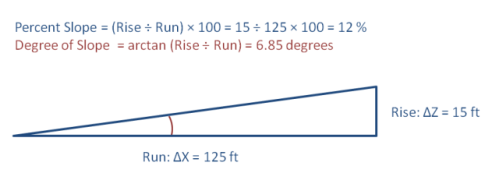
Hillshading is a technique used to visualize terrain as shaded relief, illuminating it with a hypothetical light source. The illumination value for each raster cell is determined by its orientation to the light source, which is based on slope and aspect. In the lab activity, you will experiment with placement of the light source, but, for now, it will suffice to say that positioning the light source in the northwest works best to simulate a natural landscape to the human eye. Depending on your application, you might also want to simulate the true position of the sun at a particular date and time of year.
Flood Inundation Analysis
True flood modeling, such as that used to produce FEMA's Digital Flood Insurance Rate Maps [56] (DFIRMs), is a complex process that includes terrain data, rainfall runoff or coastal storm surge models, hydrologic modeling, and hydraulic analysis. To determine the potential depth of flooding, one must be able to predict how much water is in the watershed at any given time, how that amount of water changes over time during a storm event, and how the flow of water is impeded or obstructed by vegetation or man-made structures. Floodplain mapping comprises an entire engineering discipline in its own right, and while GIS tools are extensively employed, simple topographic analysis alone does not create an accurate flood map.
That said, there may be legitimate applications for a more simple inundation analysis, such as you will perform in this lesson's lab activity. One real-world example of this was the inundation of New Orleans during Hurricane Katrina. Once the levees broke, and the water began to inundate low-lying areas of the Ninth Ward, the floodwaters were contained by the terrain features (natural and man-made) and simply rose until a steady-state condition was reached. In the end, the floodwaters were truly and accurately represented by a flat surface, and the depth of flooding could be simply determined by subtracting the land elevation at a given location from the elevation of this flat water surface. You will perform this simple type of flood inundation analysis on a land surface created from lidar point data. It will be up to you to evaluate how realistic the results are, and how they should or should not be used to predict real-world events.
Read More
You can read about modeling of the New Orleans flood in these articles:
- Gesch, Dean. Topography-based Analysis of Hurricane Katrina Inundation of New Orleans. [58] US Geological Survey.
- Griesmer et al., May 2006. Hurricane Katrina and Disaster Recovery Geospatial Process for Damage Assessment [59]. Proceedings of the 2006 American Water Resources Association Specialty Conference: GIS and Water Resources IV.
Line-of-Sight Analysis
Line-of-sight (LOS), also called "viewshed analysis," can be used to determine what can be seen from a particular location in the landscape. Conversely, the same analysis also determines from where within the surroundings that location can be seen. The first prerequisite for an LOS analysis is obviously a three-dimensional surface model of the landscape. For most applications, the most meaningful result would take vegetation, buildings, and other objects into account - those features that are purposely removed from bare-earth digital elevation models (DEMs). Above-ground features are generally included in Digital Surface Models (DSMs) created from lidar data.
LOS has many potential uses in community planning and zoning, airport operations management, event security, or battlefield cover and concealment, for example. Most students immediately think of cell phone tower placement as an application for LOS. While topography certainly has an impact on cell phone coverage, as in the case of flood inundation, modeling cell phone signal propagation [60] is in reality a much more complicated problem. An LOS analysis can be useful for planning cell-phone tower placement, but, to truly model cell phone coverage, more sophisticated models must be employed.