GEOG 489
Lesson 1 Python 3, ArcGIS Pro & Multiprocessing
1.1 Overview and Checklist
Lesson 1 is two weeks in length. The goal is to get back into Python programming with arcpy, in particular doing so under ArcGIS Pro, and learn about the concepts of parallel programming and multiprocessing and how they can be used in Python to speed up time-consumptive computations. In addition, we will discuss some important general topics related to programming such as debugging code complemented by a discussion of profiling code to detect bottlenecks, version control system software like GitHub, and different integrated development environments (IDEs) available for Python. The IDE we are going to start with in this class is called Spyder but one part of the first homework assignment will be to try out another IDE and present it in a short video.
Some sections in this lesson related to 64-bit processing for ArcGIS Desktop and code profiling are optional so that you can decide for yourself how deep you want to dive into the respective topic. The lessons in this course contain quite a lot of content, so feel absolutely free to skip these optional sections; you can always come back to check them out later or after the end of the class.
Please refer to the Calendar for specific time frames and due dates. To finish this lesson, you must complete the activities listed below. You may find it useful to print this page out first so that you can follow along with the directions.
| Step | Activity | Access/Directions |
|---|---|---|
| 1 | Engage with Lesson 1 Content | Begin with 1.2 Differences between Python 2 and Python 3 |
| 2 | Video Presentation of IDE Research | Choose the IDE you wish to research (in the IDE Investigation: Choose Topic discussion forum) and submit a video demonstration and discussion (to both the Assignment Dropbox and the Media Gallery). When picking your IDE, please take into account that we would like to see all the IDEs presented by at least one student. |
| 3 | Programming Assignment and Reflection | Submit your modified code versions and ArcGIS Pro toolboxes along with a short report (400 words) including your profiling results and a reflection on what you learned and/or what you found challenging. |
| 4 | Quiz 1 | Complete the Lesson 1 Quiz. |
| 5 | Questions/Comments | Remember to visit the Lesson 1 Discussion Forum to post/answer any questions or comments pertaining to Lesson 1 |
List of Lesson 1 Downloads
All downloads and full instructions are available and included in the Lesson 1 course material. The list below is for those who want to frontload downloading items.
Data
- USA.gdb.zip
- In section 1.6, you will also use some DEM raster data that you can download with a script we provide there. You can wait with obtaining that data until you reach that section in the lesson materials.
Software
- Spyder- Python IDE Spyder is the default IDE for Lesson 1 before we will review other IDEs at the end of the lesson and you are then free to use whichever IDE you prefer in the rest of the course. Installation instructions for Spyder can be found in Section 1.5.
Optional software: The following software will only be required if you decide to follow along the steps described in optional sections included in this lesson that contain complementary materials. We recommend that you do not install this software now, but wait until you are sure that you want to test them out.
- Optional: 64-bit processing for ArcGIS Desktop- You'll find this link on the "Optional: 64-bit Geoprocessing downloads for ArcGIS" page under Lesson 1 in Canvas. Detailed instructions can be found in Section 1.6.2.
- Optional: QCacheGRind- just unzip, don't run the .exe. See Section 1.7.2.2 for more information.
Optional Python modules
These modules are also only needed for optional materials in this lesson. So the same as said above holds here: We recommend that you do not install these now, but wait until you are sure that you want to test them out.
To install pyprof2call tree (Section 1.7.2.2)- open Python command prompt in Administrator mode and type in:
scripts\pip install pyprof2calltree
If received, ignore the message about upgrading pip.
To install line_profiler (Section 1.7.2.4)- open Python command prompt in Administrator mode and type in:
scripts\pip install line_profiler
If you receive an error that "Microsoft Visual C++ 14.0 is required", visit Microsoft's Visual Studio Downloads page and download the package for "Visual Studio Community 2017" which will download Visual Studio Installer. Run Visual Studio Installer, and under the "Workloads" tab, you will select two components to install. Under Windows, check the box in the upper right-hand corner of "Desktop Development with C++," and under Web & Cloud, check the box for "Python development". After checking the boxes, click "Install" in the lower right-hand corner. After installing those, open the Python command prompt again and enter:
scripts\pip install misaka
If that works, then install the line_profiler with...
scripts\pip install line_profiler
You should see a message saying “Successfully installed line-profiler-2.1.2" although your version number may be different and that’s okay.
1.2 Differences between Python 2 and Python 3
If you have taken GEOG 485 before we changed it from ArcGIS Desktop to Pro or you learned about Python programming and customization of ArcGIS Desktop in some other context, then you have been working with arcpy under Python version 2. ArcPy is also available in ArcGIS Pro, but everything here runs under Python version 3. This is why we start this first lesson of the course with an overview on the differences between Python 2 and Python 3.
Python 3.0 was released in 2008 and the final version of 2.7 was released in mid-2010, so they have both been around for a long time. There are no major developments planned for Python 2, with all the attention focused on Python 3.
While a lot of the changes from Python 2 to Python 3 were in the background or with special features that we won’t need in this course, there are a few changes that you are somewhat likely to encounter and that we, therefore, list on the following pages.
In addition, while many things in the ArcGIS Pro version of arcpy still work in the same way as in the version you might know from ArcGIS Desktop, there are some differences, in particular with respect to the availability of certain modules and tools. This won’t be a concern in this first lesson, but we will examine the differences in the following section.
You might wonder why we're talking about old versions of Python and ArcGIS Desktop and it's a fair question. At some point, you may want to run some pre-existing Python 2 code in ArcGIS Pro for any number of reasons that might include updating legacy tools, converting old code, using new ArcGIS Pro tools, sharing with ArcGIS Pro users, using Python 3 libraries, importing a legacy MXD from ArcGIS Desktop or perhaps using the better performance, which may come from using either multiprocessing or 64 bit processing (although these are also available in Python 2 and you can experiment with those later in the lesson). There's a reasonable chance you're going to be exposed to this older Python 2 code at some point and when that happens we want you to know how to update it easily.
print ... vs. print(...)
There are several differences between Python 2 and 3, but the most obvious one is that the print statement from Python 2 is now a function in 3. You might recall from GEOG 485 that a function takes parameters (and sometimes returns a value).
Have a look at the example below for a simple illustration of this change. You’ll notice that for Python 2 both will work. Usually, though, most people have written code using the standard Python 2 print statement, not the way which appears to support print as a function.
#Python 2
print "Hello World"
print ("Hello World")
#Python 3
print ("Hello World")
All of the more complicated things that we can do with a print statement such as adding in variables or using the .format statement can be implemented just the same. If you're unfamiliar with .format we will look at it in more detail soon.
#Python 2
Name = "James"
print "Hello World. My name is " + Name
print "Hello World. My name is {0}".format(Name)
#Python 3
Name = "James"
print ("Hello World. My name is " + Name)
print ("Hello World. My name is {0}".format(Name))
You can experiment with creating more complicated versions of those print statements or functions depending on which version of Python you’re using. In the class, if we’re describing print, we will be using the terms statement and function interchangeably – be sure to adjust your code according to the version of Python you’re using. Be aware that you can use the Python 3 version in Python 2.7 and many programmers have transitioned to using this approach over time (but you'll potentially still see print used as per our Python 2 examples above).
For the technically-minded, I mentioned above that in Python 2 print appears to work as a function but it’s actually being interpreted by Python as (“Hello World”) which is equivalent to “Hello World” in Python.
Integer division
In Python 2, the result of a division between two integer numbers was again an integer number, namely the result with everything after the decimal point truncated. So for instance, the result of the expression
1 / 2
is the integer number 0. If you wanted to have the result as a floating point number you had to use something like 1 / float(2) or 1 / 2.0 to first turn one of the operands into a float. This behavior has changed in Python 3. The result is now a floating point number, so 0.5 in this case.
Strings
Python 2 had two different string data types, str() for ASCII strings (so only providing for a very limited set of different characters but also only requiring one byte per character) and unicode() for Unicode strings allowing for a much larger set of characters and supporting writings that are not Latin-based such as Chinese characters for example. To create a Unicode string you had to use the prefix u like this: u'some string'. You might remember this u appearing in front of some output in Python 2, for instance from arcpy functions such as ListFeatureClasses().
In Python 3, everything within quotes is considered a unicode UTF-8 string, so you can write
print('Saying hello in Chinese: 你好')
As in Python 2, Unicode characters can be written with a \u followed by their 4 or 8 digit hexadecimal number if you have no other way of entering the characters into the code. So the previous command can also be written as:
print('Saying hello in Chinese: \u4f60\u597d')
In case you have not heard much about the Unicode standard for encoding characters, here is a good article explaining what this is all about: A Beginner-Friendly Guide to Unicode.
Reorganization of the Python standard library
With the change to Python 3, the modules from the standard library have been reorganized. As a result, the import statements used in a Python 2 script may not work anymore because the names of modules have changed, etc. For instance, in Python 2 the standard library contains the modules urllib and urllib2 for working with URLs and accessing content on the web. In Python 3, the functionality has been reorganized into three submodules called urllib.parse, urllib.request, and urllib.error. There are more examples like this and also examples of individual functions or classes that have a changed name or have been removed entirely.
If you want to dive deeper into this topic, have a look at the page "What's New in Python 3.0" from the Python documentation and this article summarizing the key differences between Python 2 and 3.
Differences between ArcGIS Desktop and ArcGIS Pro's arcpy functions.
There are some differences in the level of functionality available in arcpy in Desktop when compared to Pro. These are documented in the Pro help here and here. Probably the one most likely to trip up those of you with existing scripts is the renaming of arcpy.mapping to arcpy.mp which will require some changes to code (including any function calls to arcpy.mapping.<name> functions).
There is also a list of tools which are not supported in Pro which aren't commonly used but could have specialty tools that rely on them. These tools include Coverage (arcpy.arc), Data Interoperability (arcpy.interop), Parcel Fabric (arcpy.fabric), Schematics (arcpy.schematics), and Tracking Analyst (arcpy.ta). If you're migrating from Desktop to Pro in your professional lives, it might be worthwhile checking that none of your scripts or workflows require these tools.
In addition to these entire toolboxes which are no longer available in Pro, a number of individual tools within toolboxes have either not been implemented or haven't been implemented yet. We won't repeat that long list here, but it may be worth having a quick look over the list (this is the second link from two paragraphs above) to double-check that any of your necessary or favorite tools aren't in the list.
There are also both new and improved tools within Pro that don't exist within Desktop. Some of these take advantage of parallel processing or are written more efficiently and therefore perform better than their legacy (old) versions. When using Pro you'll often see a small tooltip in the top of the Geoprocessing window mentioning that another tool offers improved performance or additional functionality.
1.3 Import & loops revisited, and some syntactic sugar
To warm up a bit, let’s briefly revisit a few Python features that you are already familiar with but for which there exist some forms or details that you may not yet know, starting with the Python “import” command. We are also going to introduce a few Python constructs that you may not have heard about yet on the way.
It is highly recommended that you try out these examples yourself and experiment with them to get a better understanding. The examples work in both Python 2 and Python 3, so you can use any Python installation and IDE that you have on your computer for this. If you are not sure what to use, you can also look ahead at the part of Section 1.5 about getting a Python 3 IDE for ArcGIS Pro, spyder, up and running and then come back to this section here.
1.3.1 Import
The form of the “import” command that you definitely should already know is
import <module name>
e.g.,
import arcpy
What happens here is that the module (either a module from the standard library, a module that is part of another package you installed, or simply another .py file in your project directory) is loaded, unless it has already been loaded before, and the name of the module becomes part of the namespace of the script that contains the import command. As a result, you can now access all variables, functions, or classes defined in the imported module, by writing
<module name>.<variable or function name>
e.g.,
arcpy.Describe(…)
You can also use the import command like this instead:
import arcpy as ap
This form introduces a new alias for the module name, typically to save some typing when the module name is rather long, and instead of writing
arcpy.Describe(…)
, you would now use
ap.Describe(…)
in your code.
Another approach of using “import” is to directly add content of a module (again either variables, functions, or classes) to the namespace of the importing Python script. This is done by using the form "from … import …" as in the following example:
from arcpy import Describe, Point , …

...

Describe(…)
The difference is that now you can use the imported names directly in our code without having to use the module name (or an alias) as a prefix as it is done in line 5 of the example code. However, be aware that if you are importing multiple modules, this can easily lead to name conflicts if, for instance, two modules contain functions with the same name. It can also make your code a little more difficult to read since
arcpy.Describe(...)
helps you or another programmer recognize that you’re using something defined in arcpy and not in another library or the main code of your script.
You can also use
from arcpy import *
to import all variable, function and class names from a module into the namespace of your script if you don’t want to list all those you actually need. However, this can increase the likelihood of a name conflict.
1.3.2 Loops, continue, break
Next, let’s quickly revisit loops in Python. There are two kinds of loops in Python, the for-loop and the while-loop. You should know that the for-loop is typically used when the goal is to go through a given set or list of items or do something a certain number of times. In the first case, the for-loop typically looks like this
for item in list:

    # do something with item
while in the second case, the for-loop is often used together with the range(…) function to determine how often the loop body should be executed:
for i in range(50):

	# do something 50 times
In contrast, the while-loop has a condition that is checked before each iteration and if the condition becomes False, the loop is terminated and the code execution continues after the loop body. With this knowledge, it should be pretty clear what the following code example does:
import random

r = random.randrange(100) # produce random number between 0 and 99

attempts = 1

while r != 11:

    attempts += 1

    r = random.randrange(100)

print('This took ' + str(attempts) + ' attempts')
What you may not yet know is that there are two additional commands, break and continue, that can be used in combination with either a for or a while-loop. The break command will automatically terminate the execution of the current loop and continue with the code after it. If the loop is part of a nested loop only the inner loop will be terminated. This means we can rewrite the program from above using a for-loop rather than a while-loop like this:
import random

attempts = 0

for i in range(1000):

    r = random.randrange(100)

    attempts += 1

    if r == 11:

        break  # terminate loop and continue after it

print('This took ' + str(attempts) + ' attempts')
When the random number produced in the loop body is 11, the body of the if-statement, so the break command, will be executed and the program execution immediately leaves the loop and continues with the print statement after it. Obviously, this version is not completely identical to the while based version from above because the loop will be executed at most 1000 times here.
If you have experience with programming languages other than Python, you may know that some languages have a "do … while" loop construct where the condition is only tested after each time the loop body has been executed so that the loop body is always executed at least once. Since we first need to create a random number before the condition can be tested, this example would actually be a little bit shorter and clearer using a do-while loop. Python does not have a do-while loop but it can be simulated using a combination of while and break:
import random

attempts = 0

while True:

    r = random.randrange(100)

    attempts += 1

    if r == 11:

        break

print('This took ' + str(attempts) + ' attempts')
A while loop with the condition True will in principle run forever. However, since we have the if-statement with the break, the execution will be terminated as soon as the random number generator rolls an 11. While this code is not shorter than the previous while-based version, we are only creating random numbers in one place, so it can be considered a little bit more clear.
When a continue command is encountered within the body of a loop, the current execution of the loop body is also immediately stopped, but in contrast to the break command, the execution then continues with the next iteration of the loop body. Of course, the next iteration is only started if, in the case of a while-loop, the condition is still true, or in the case of a for-loop, there are still remaining items in the list that we are looping through. The following code goes through a list of numbers and prints out only those numbers that are divisible by 3 (without remainder).
l = [3,7,99,54,3,11,123,444]

for n in l:

    if n % 3 != 0:   # test whether n is not divisible by 3 without remainder

        continue

    print(n)
This code uses the modulo operator % to get the remainder of the division of n and 3 in line 5. If this remainder is not 0, the continue command is executed and, as a result, the program execution directly jumps back to the beginning of the loop and continues with the next number. If the condition is False (meaning the number is divisible by 3), the execution continues as normal after the if-statement and prints out the number. Hopefully, it is immediately clear that the same could have been achieved by changing the condition from != to == and having an if-block with just the print statement, so this is really just a toy example illustrating how continue works.
As you saw in these few examples, there are often multiple ways in which for, while, break, continue, and if-else can be combined to achieve the same thing. While break and continue can be useful commands, they can also make code more difficult to read and understand. Therefore, they should only be used sparingly and when their usage leads to a simpler and more comprehensible code structure than a combination of for /while and if-else would do.
1.3.3 Expressions and the "...if ... else ..." ternary operator
You are already familiar with Python binary operators that can be used to define arbitrarily complex expressions. For instance, you can use arithmetic expressions that evaluate to a number, or boolean expressions that evaluate to either True or False. Here is an example of an arithmetic expression using the arithmetic operators – and *:
x = 25 – 2 * 3
Each binary operator takes two operand values of a particular type (all numbers in this example) and replaces them by a new value calculated from the operands. All Python operators are organized into different precedence classes, determining in which order the operators are applied when the expression is evaluated unless parentheses are used to explicitly change the order of evaluation. This operator precedence table shows the classes from lowest to highest precedence. The operator * for multiplication has a higher precedence than the – operator for subtraction, so the multiplication will be performed first and the result of the overall expression assigned to variable x is 19.
Here is an example for a boolean expression:
x = y > 12 and z == 3
The boolean expression on the right side of the assignment operator contains three binary operators: two comparison operators, > and ==, that take two numbers and return a boolean value, and the logical ‘and’ operator that takes two boolean values and returns a new boolean (True only if both input values are True, False otherwise). The precedence of ‘and’ is lower than that of the two comparison operators, so the ‘and’ will be evaluated last. So if y has the value 6 and z the value 3, the value assigned to variable x by this expression will be False because the comparison on the left side of the ‘and’ evaluates to False.
In addition to all these binary operators, Python has a ternary operator, so an operator that takes three operands as input. This operator has the format
x if c else y
x, y, and c here are the three operands while ‘if’ and ‘else’ are the keywords making up the operator and demarcating the operands. While x and y can be values or expressions of arbitrary type, the condition c needs to be a boolean value or expression. What the operator does is it looks at the condition c and if c is True it evaluates to x, else it evaluates to y. So for example in the following line of code
p = 1 if x > 12 else 0
variable p will be assigned the value 1 if x is larger than 12, else p will be assigned the value 0. Obviously what the ternary if-else operator does is very similar to what we can do with an if or if-else statement. For instance, we could have written the previous code as
p = 1

if x > 12:

    p = 0
The “x if c else y” operator is an example of a language construct that does not add anything principally new to the language but enables writing things more compactly or more elegantly. That’s why such constructs are often called syntactic sugar. The nice thing about “x if c else y” is that in contrast to the if-else statement, it is an operator that evaluates to a value and, hence, can be embedded directly within more complex expressions as in the following example that uses the operator twice:
newValue = 25 + (10 if oldValue < 20 else 44) / 100 + (5 if useOffset else 0)
Using an if-else statement for this expression would have required at least five lines of code.
1.3.4 String concatenation vs. format
In GEOG 485, we used the + operator for string concatenation to produce strings from multiple components to then print them out or use them in some other way, as in the following two examples:
print('The feature class contains ' + str(n) + ' point features.')

queryString = '"'+ fieldName+ '" = ' + "'" + countryName + "'"
An alternative to this approach using string concatenation is to use the string method format(…). When this method is invoked for a particular string, the string content is interpreted as a template in which parts surrounded by curly brackets {…} should be replaced by the variables given as parameters to the method. Here is how the two examples from above would look in this approach:
print('The feature class contains {0} point features.'.format(n) )

queryString = '"{0}" = \'{1}\''.format(fieldName, countryName)
In both examples, we have a string literal '….' and then directly call the format(…) method for this string literal to give us a new string in which the occurrences of {…} have been replaced. In the simple form {i} used here, each occurrence of this pattern will be replaced by the i-th parameter given to format(…). In the second example, {0} will be replaced by the value of variable fieldName and {1} will be replaced by variable countryName. Please note that the second example will also use \' to produce the single quotes so that the entire template could be written as a single string. The numbers within the curly brackets can also be omitted if the parameters should be inserted into the string in the order in which they appear.
The main advantages of using format(…) are that the string can be a bit easier to produce and read as in particular in the second example, and that we don’t have to explicitly convert all non-string variables to strings with str(…). In addition, format allows us to include information about how the values of the variables should be formatted. By using {i:n}, we say that the value of the i-th variable should be expanded to n characters if it’s less than that. For strings, this will by default be done by adding spaces after the actual string content, while for numbers, spaces will be added before the actual string representation of the number. In addition, for numbers, we can also specify the number d of decimal digits that should be displayed by using the pattern {i:n.df}. The following example shows how this can be used to produce some well-formatted list output:
items = [('Maple trees', 45.232 ),  ('Pine trees', 30.213 ), ('Oak trees', 24.331)]

for i in items:

    '{0:20} {1:3.2f}%'.format(i[0], i[1])
Output:
Maple trees                          45.23%
Pine trees                           30.21%
Oak trees                            24.33%
The pattern {0:20} is used here to always fill up the names of the tree species in the list with spaces to get 20 characters. Then the pattern {1:3.2f} is used to have the percentage numbers displayed as three characters before the decimal point and two digits after. As a result, the numbers line up perfectly.
The format method can do a few more things, but we are not going to go into further details here. Check out this page about formatted output if you would like to learn more about this.
1.4 Functions revisited
From GEOG 485 or similar previous experience, you should be familiar with defining simple functions that take a set of input parameters and potentially return some value. When calling such a function from somewhere in your Python code, you have to provide values (or expressions that evaluate to some value) for each of these parameters, and these values are then accessible under the names of the respective parameters in the code that makes up the body of the function.
However, from working with different tool functions provided by arcpy and different functions from the Python standard library, you also already know that functions can also have optional parameters, and you can use the names of such parameters to explicitly provide a value for them when calling the function. In this section, we will show you how to write functions with such keyword arguments and functions that take an arbitrary number of parameters, and we will discuss some more details about passing different kinds of values as parameters to a function.
1.4.1 Functions with keyword arguments
The parameters we have been using so far, for which we only specify a name in the function definition, are called positional parameters or positional arguments because the value that will be assigned to them when the function is called depends on their position in the parameter list: The first positional parameter will be assigned the first value given within the parentheses (…) when the function is called, and so on. Here is a simple function with two positional parameters, one for providing the last name of a person and one for providing a form of address. The function returns a string to greet the person with.
def greet(lastName, formOfAddress):

      return 'Hello {0} {1}!'.format(formOfAddress, lastName)


print(greet('Smith', 'Mrs.'))
Output:

Hello Mrs. Smith!
Note how the first value used in the function call (“Smith”) in line 6 is assigned to the first positional parameter (lastName) and the second value (“Mrs.”) to the second positional parameter (formOfAddress). Nothing new here so far.
The parameter list of a function definition can also contain one or more so-called keyword arguments. A keyword argument appears in the parameter list as
<argument name> = <default value>
A keyword argument can be provided in the function by again using the notation
def greet(lastName, formOfAddress, language = 'English'):

      greetings = { 'English': 'Hello', 'Spanish': 'Hola' }

      return '{0} {1} {2}!'.format(greetings[language], formOfAddress, lastName)


print(greet('Smith', 'Mrs.'))

print(greet('Rodriguez', 'Sr.', language = 'Spanish'))
Output:

Hello Mrs. Smith!
Hola Sr. Rodriguez!
Compare the two different ways in which the function is called in lines 8 and 10. In line 8, we do not provide a value for the ‘language’ parameter so the default value ‘English’ is used when looking up the proper greeting in the dictionary stored in variable greetings. In the second version in line 10, the value ‘Spanish’ is provided for the keyword argument ‘language,’ so this is used instead of the default value and the person is greeted with “Hola” instead of "Hello." Keyword arguments can be used like positional arguments meaning the second call could also have been
print(greet('Rodriguez', 'Sr.', 'Spanish'))
without the “language =” before the value.
Things get more interesting when there are several keyword arguments, so let’s add another one for the time of day:
def greet(lastName, formOfAddress, language = 'English', timeOfDay = 'morning'):

      greetings = { 'English': { 'morning': 'Good morning', 'afternoon': 'Good afternoon' },

                    'Spanish': { 'morning': 'Buenos dias', 'afternoon': 'Buenas tardes' } }

      return '{0}, {1} {2}!'.format(greetings[language][timeOfDay], formOfAddress, lastName)


print(greet('Smith', 'Mrs.'))

print(greet('Rodriguez', 'Sr.', language = 'Spanish', timeOfDay = 'afternoon'))
Output:

Good morning, Mrs. Smith!
Buenas tardes, Sr. Rodriguez!
Since we now have four different forms of greetings depending on two parameters (language and time of day), we now store these in a dictionary in variable greetings that for each key (= language) contains another dictionary for the different times of day. For simplicity reasons, we left it at two times of day, namely “morning” and “afternoon.” In line 7, we then first use the variable language as the key to get the inner dictionary based on the given language and then directly follow up with using variable timeOfDay as the key for the inner dictionary.
The two ways we are calling the function in this example are the two extreme cases of (a) providing none of the keyword arguments, in which case default values will be used for both of them (line 10), and (b) providing values for both of them (line 12). However, we could now also just provide a value for the time of day if we want to greet an English person in the afternoon:
print(greet('Rogers', 'Mrs.', timeOfDay = 'afternoon'))
Output:

Good afternoon, Mrs. Rogers!
This is an example in which we have to use the prefix “timeOfDay =” because if we leave it out, it will be treated like a positional parameter and used for the parameter ‘language’ instead which will result in an error when looking up the value in the dictionary of languages. For similar reasons, keyword arguments must always come after the positional arguments in the definition of a function and in the call. However, when calling the function, the order of the keyword arguments doesn’t matter, so we can switch the order of ‘language’ and ‘timeOfDay’ in this example:
print(greet('Rodriguez', 'Sr.', timeOfDay = 'afternoon', language = 'Spanish'))
Of course, it is also possible to have function definitions that only use optional keyword arguments in Python.
1.4.2 Functions with an arbitrary number of parameters
Let us continue with the “greet” example, but let’s modify it to be a bit simpler again with a single parameter for picking the language, and instead of using last name and form of address we just go with first names. However, we now want to be able to not only greet a single person but arbitrarily many persons, like this:
greet('English', 'Jim', 'Michelle')
Output:

Hello Jim!
Hello Michelle!
greet('Spanish', 'Jim', 'Michelle', 'Sam')
Output:

Hola Jim!
Hola Michelle!
Hola Sam!
To achieve this, the parameter list of the function needs to end with a special parameter that has a * symbol in front of its name. If you look at the code below, you will see that this parameter is treated like a list in the body of the function:
def greet(language, *names):

     greetings = { 'English': 'Hello', 'Spanish': 'Hola' }

     for n in names:

          print('{0} {1}!'.format(greetings[language], n))
What happens is that all values given to that function from the one corresponding to the parameter with the * on will be placed in a list and assigned to that parameter. This way you can provide as many parameters as you want with the call and the function code can iterate through them in a loop. Please note that for this example we changed things so that the function directly prints out the greetings rather than returning a string.
We also changed language to a positional parameter because if you want to use keyword arguments in combination with an arbitrary number of parameters, you need to write the function in a different way. You then need to provide another special parameter starting with two stars ** and that parameter will be assigned a dictionary with all the keyword arguments provided when the function is called. Here is how this would look if we make language a keyword parameter again:
def greet(*names, **kwargs):

     greetings = { 'English': 'Hello', 'Spanish': 'Hola' }

     language = kwargs['language'] if 'language' in kwargs else 'English'

     for n in names:

          print('{0} {1}!'.format(greetings[language], n))
If we call this function as
greet('Jim', 'Michelle')
the output will be:
Hello Jim!
Hello Michelle!
And if we use
greet('Jim', 'Michelle', 'Sam', language = 'Spanish')
we get:
Hola Jim!
Hola Michelle!
Hola Sam!
Yes, this is getting quite complicated, and it’s possible that you will never have to write functions with both * and ** parameters, still here is a little explanation: All non-keyword parameters are again collected in a list and assigned to variable names. All keyword parameters are placed in a dictionary using the name appearing before the equal sign as the key, and the dictionary is assigned to variable kwargs. To really make the ‘language’ keyword argument optional, we have added line 5 in which we check if something is stored under the key ‘language’ in the dictionary (this is an example of using the ternary "... if ... else ..." operator). If yes, we use the stored value and assign it to variable language, else we instead use ‘English’ as the default value. In line 9, language is then used to get the correct greeting from the dictionary in variable greetings while looping through the name list in variable names.
1.4.3 Local vs. global, mutable vs. immutable
When making the transition from a beginner to an intermediate or advanced Python programmer, it also gets important to understand the intricacies of variables used within functions and of passing parameters to functions in detail. First of all, we can distinguish between global and local variables within a Python script. Global variables are defined outside of any function. They can be accessed from anywhere in the script and they exist and keep their values as long as the script is loaded which typically means as long as the Python interpreter into which they are loaded is running.
In contrast, local variables are defined inside a function and can only be accessed in the body of that function. Furthermore, when the body of the function has been executed, its local variables will be discarded and cannot be used anymore to access their current values. A local variable is either a parameter of that function, in which case it is assigned a value immediately when the function is called, or it is introduced in the function body by making an assignment to the name for the first time.
Here are a few examples to illustrate the concepts of global and local variables and how to use them in Python.
def doSomething(x):      # parameter x is a local variable of the function

     count = 1000 * x    # local variable count is introduced

     return count


y = 10            # global variable y is introduced

print(doSomething(y))

print(count)      # this will result in an error

print(x)          # this will also result in an error
This example introduces one global variable, y, and two local variables, x and count, both part of the function doSomething(…). x is a parameter of the function, while count is introduced in the body of the function in line 3. When this function is called in line 11, the local variable x is created and assigned the value that is currently stored in global variable y, so the integer number 10. Then the body of the function is executed. In line 3, an assignment is made to variable count. Since this variable hasn’t been introduced in the function body before, a new local variable will now be created and assigned the value 10000. After executing the return statement in line 5, both x and count will be discarded. Hence, the two print statements at the end of the code would lead to errors because they try to access variables that do not exist anymore.
Now let’s change the example to the following:
def doSomething():

     count = 1000 * y    # global variable y is accessed here

     return count


y = 10

print(doSomething())
This example shows that global variable y can also be directly accessed from within the function doSomething(): When Python encounters a variable name that is neither the name of a parameter of that function nor has been introduced via an assignment previously in the body of that function, it will look for that variable among the global variables. However, the first version using a parameter instead is usually preferable because then the code in the function doesn’t depend on how you name and use variables outside of it. That makes it much easier to, for instance, re-use the same function in different projects.
So maybe you are wondering whether it is also possible to change the value of a global variable from within a function, not just read its value? One attempt to achieve this could be the following:
 def doSomething():

     count = 1000

     y = 5

     return count * y


y = 10

print(doSomething())

print(y)      # output will still be 10 here
However, if you run the code, you will see that last line still produces the output 10, so the global variable y hasn't been changed by the assignment in line 5. That is because the rule is that if a name is encountered on the left side of an assignment in a function, it will be considered a local variable. Since this is the first time an assignment to y is made in the body of the function, a new local variable with that name is created at that point that will overshadow the global variable with the same name until the end of the function has been reached. Instead, you explicitly have to tell Python that a variable name should be interpreted as the name of a global variable by using the keyword ‘global’, like this:
def doSomething():

     count = 1000

     global y      # tells Python to treat y as the name of global variable

     y = 5         # as a result, global variable y is assigned a new value here

     return count * y


y = 10

print(doSomething())

print(y)       # output will now be 5 here
In line 5, we are telling Python that y in this function should refer to the global variable y. As a result, the assignment in line 7 changes the value of the global variable called y and the output of the last line will be 5. While it's good to know how these things work in Python, we again want to emphasize that accessing global variables from within functions should be avoided as much as possible. Passing values via parameters and returning values is usually preferable because it keeps different parts of the code as independent of each other as possible.
So after talking about global vs. local variables, what is the issue with mutable vs. immutable mentioned in the heading? There is an important difference in passing values to a function depending on whether the value is from a mutable or immutable data type. All values of primitive data types like numbers and boolean values in Python are immutable, meaning you cannot change any part of them. On the other hand, we have mutable data types like lists and dictionaries for which it is possible to change their parts: You can, for instance, change one of the elements in a list or what is stored under a particular key in a given dictionary without creating a completely new object.
What about strings and tuples? You may think these are mutable objects, but they are actually immutable. While you can access a single character from a string or element from a tuple, you will get an error message if you try to change it by using it on the left side of the equal sign in an assignment. Moreover, when you use a string method like replace(…) to replace all occurrences of a character by another one, the method cannot change the string object in memory for which it was called but has to construct a new string object and return that to the caller.
Why is that important to know in the context of writing functions? Because mutable and immutable data types are treated differently when provided as a parameter to functions as shown in the following two examples:
def changeIt(x):

     x = 5   # this does not change the value assigned to y


y = 3

changeIt(y)

print(y)     # will print out 3
As we already discussed above, the parameter x is treated as a local variable in the function body. We can think of it as being assigned a copy of the value that variable y contains when the function is called. As a result, the value of the global variable y doesn’t change and the output produced by the last line is 3. But it only works like this for immutable objects, like numbers in this case! Let’s do the same thing for a list:
def changeIt(x):

     x[0] = 5   # this will change the list y refers to


y = [3,5,7]

changeIt(y)

print(y)        # output will be [5, 5, 7]
The output [5,5,7] produced by the print statement in the last line shows that the assignment in line 3 changed the list object that is stored in global variable y. How is that possible? Well, for values of mutable data types like lists, assigning the value to function parameter x cannot be conceived as creating a copy of that value and, as a result, having the value appear twice in memory. Instead, x is set up to refer to the same list object in memory as y. Therefore, any change made with the help of either variable x or y will change the same list object in memory. When variable x is discarded when the function body has been executed, variable y will still refer to that modified list object. Maybe you have already heard the terms “call-by-value” and “call-by-reference” in the context of assigning values to function parameters in other programming languages. What happens for immutable data types in Python works like “call-by-value,” while what happens to mutable data types works like “call-by-reference.” If you feel like learning more about the details of these concepts, check out this article on Parameter Passing.
While the reasons behind these different mechanisms are very technical and related to efficiency, this means it is actually possible to write functions that take parameters of mutable type as input and modify their content. This is common practice (in particular for class objects which are also mutable) and not generally considered bad style because it is based on function parameters and the code in the function body does not have to know anything about what happens outside of the function. Nevertheless, often returning a new object as the return value of the function rather than changing a mutable parameter is preferable. This brings us to the last part of this section.
1.4.4 Multiple return values
It happens quite often that you want to hand back different things as the result of a function, for instance four coordinates describing the bounding box of a polygon. But a function can only have one return value. It is common practice in such situations to simply return a tuple with the different components you want to return, so in this case a tuple with the four coordinates. Python has a useful mechanism to help with this by allowing us to assign the elements of a tuple (or other sequences like lists) to several variables in a single assignment. Given a tuple t = (12,3,2,2), instead of writing
top = t[0]

left = t[1]

bottom = t[2]

right = t[3]
you can write
top, left, bottom, right = t
and it will have the exact same effect. The following example illustrates how this can be used with a function that returns a tuple of multiple return values. For simplicity, the function computeBoundingBox() in this example only returns a fixed tuple rather than computing the actual tuple values from a polygon given as input parameter.
def computeBoundingBox():

     return (12,3,41,32)


top, left, bottom, right = computeBoundingBox() # assigns the four elements of the returned tuple to individual variables

print(top)    # output: 12
This section has been quite theoretical, but you will often encounter the constructs presented here when reading other people’s Python code and also in the rest of this course.
1.5 Working with Python 3 and arcpy in ArcGIS Pro
Now that we’re all warmed up with some Python revision and a few clues about the changes between Python 2 and 3, we’ll start getting familiar with Python 3 in ArcGIS Pro by exploring how we write code and deploy tools just like we did when we started out in GEOG 485.
We’ll cover the conda environment that ArcGIS Pro uses for Python 3 in more detail in Lesson 2, but for now it might be helpful to think of conda as a box or container that Python 3 and all of its parts sit inside. In order to access Python 3, we’ll need to open the conda box, and to do that we will need a command prompt with administrator privileges.
Installing spyder
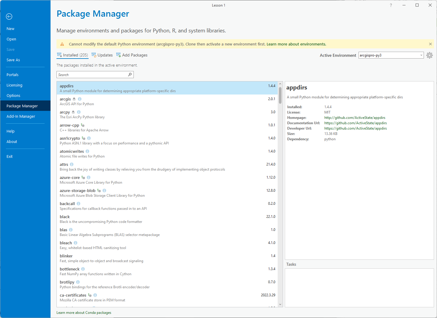
Spyder is the easiest IDE to install for Python 3 development as we can install it from ArcGIS Pro. Within Pro, you can navigate to the "Project" menu and then choose "Python" to access the Python package and environment manager of the ArcGIS Pro installation.
Since version 2.3 of ArcGIS Pro, it is not possible to modify the default Python environment anymore (see here for details). If you already have a working Pro + Spyder setup (e.g. from Geog485) and it is at least Pro version 2.7, you can keep using this installation for this class. Else I'd recommend you work with the newest version, so you will first have to create a clone of Pro's default Python environment and make it the active environment of ArcGIS before installing Spyder. In the past, students sometimes had problems with the cloning operation that we were able to solve by running Pro in admin mode.
Therefore, we recommend that before performing the following steps, you exit Pro and restart it in admin mode by doing a right-click -> Run as administrator. Then go back to "Project" -> "Python", click on "Manage Environments", and then click on "Clone Default" in the Manage Environments dialog that opens up. Installing the clone will take some time (you can watch the individual packages being installed within the "Manage Environments" window and you may be prompted to restart ArcGIS Pro to effect your changes); when it's done, the new environment "arcgispro-py3-clone" (or whatever you choose to call it - but we'll be assuming it's called the default name) can be activated by clicking on the button on the left.
Do so and also note down the path where the cloned environment has been installed appearing below the name. It should be something like C:\Users\<username>\AppData\Local\ESRI\conda\envs\arcgispro-py3-clone . Then click the OK button.
Important: The cloned environment will most likely become unusable when you update Pro to a newer main version (e.g. from 2.9 to 3.0 or 3.0 to 3.1). So once you have cloned the environment successfully, please don't update your Pro installation before the end of the class, unless you are willing to do the cloning and spyder installation again. There is a function in V3.x and later of Pro to update your Python installation but it's new functionality so it might not yet always work as expected.
Now back at the package manager, the new Python environment should appear under "Project Environment" as shown in the figure below (but be aware this might take 30+ minutes so you'll need to be patient).
To now install Spyder, select "Add Packages," search for Spyder and click the "Install" button. This might also take around 30+ minutes and it'll be best if you've restarted Pro after creating your new environment and selecting it.
The package manager will show you a list of packages that will have to be installed and ask you to agree to the terms and conditions. After doing that, the installation will start and probably take a while. You may also get get a "User Access Control" window popup asking if you want conda_uac.exe to make changes to your device; it is OK to choose Yes.
Once the installation is finished, it is recommended that you restart ArcGIS Pro (and if you have trouble restart your PC as well it usually helps). If you keep having problems with the installation failing or Spyder simply not showing up in the list of installed pacakges (even after refereshing the list), please try with starting ArcGIS Pro in admin mode (if you are not already running it this way) by doing a right-click -> Run as administrator.
Once Spyder is installed, you might like to create a shortcut to it on your Desktop or Start Menu. In that case, you should be able to find the Spyder executable in the Scripts subfolder of your cloned Python environment, so at C:\Users\<username>\AppData\Local\ESRI\conda\envs\arcgispro-py3-clone\Scripts\spyder.exe where <username> needs to be replaced with your Windows user name. f you don't see the AppData folder, you will have to change the options in the Windows File Explorer to display hidden files and folders. Make sure to use the .exe file called spyder.exe, not the one called spyder3.exe . If you are using an older version of ArcGIS Pro and installed Spyder directly into the default environment, the path will most likely be C:\Program Files\ArcGIS\Pro\bin\Python\envs\arcgispro-py3\Scripts\spyder.exe .
If you are familiar with another IDE, you're welcome to substitute it for Spyder (just verify that it is using Python 3).
When Spyder launches, it may ask you whether you want to update to a newer version. We recommend to NOT try this because the update procedure will most likely not work with the ArcGIS Pro Python environment. Once Spyder is started, it should display a message in the IPython tab similar to:
Python 3.6.2 |Continuum Analytics, Inc.| (default, Jul 20 2017, 12:30:02) [MSC v.1900 64 bit (AMD64)] Type "copyright", "credits" or "license" for more information. IPython 6.3.1 -- An enhanced Interactive Python.
In [1]:
Don’t worry if the version number is different, as long as it starts with a 3. What we’re looking at here is equivalent to the Python interactive window in ArcGIS Desktop, ArcGIS Pro, PythonWin or any of the IDEs you might be familiar with.
We can experiment here by typing "import arcpy" to import arcpy or running some of those print statement examples from earlier.
In [1]: import arcpy
In [2]: print ("Hello World")
Hello world
You might have noticed while typing in that second example a useful function of the IPython interactive window - code completion. This is where the IDE (spyder does it too) is smart enough to recognize that you're entering a function name and it provides you with the information about the parameters that function takes. If you missed it the first time, enter print( in the IPython window and wait for a second (or less) and the print function's parameters will appear. This also works for arcpy functions (or those from any library that you import). Try it out with arcpy.management.CreateFeatureclass(or your favorite arcpy function).
A first arcpy code example
Click the File menu -> New File option to open a blank code editor window that we can use to write our first piece of Python 3 code with the ArcGIS Pro version of arcpy. In the remainder of this lesson, we’re going to look at some simple examples taken from GEOG 485 (because they should be somewhat familiar to most people) which we’ll use to practice modifying code from Python 2 to 3 where needed and working with arcpy under ArcGIS Pro. Later, we’ll use some of these same code examples to migrate from single processor, sequential execution to multiprocessor, parallel execution. Below, we show the "old" Python 2 version of the code followed by the Python 3 version that you can try out in spyder, e.g. by copying the code into an empty editor window and running it from there.
This first example script reports the spatial reference (coordinate system) of a feature class stored in a geodatabase:
# Opens a feature class from a geodatabase and prints the spatial reference

import arcpy

featureClass = "C:/Data/USA/USA.gdb/States"

# Describe the feature class and get its spatial reference
desc = arcpy.Describe(featureClass)
spatialRef = desc.spatialReference

# Print the spatial reference name
print spatialRef.Name
Python 3 / ArcGIS Pro version:
# Opens a feature class from a geodatabase and prints the spatial reference

import arcpy

featureClass = "C:/Data/USA/USA.gdb/States"

# Describe the feature class and get its spatial reference
desc = arcpy.Describe(featureClass)
spatialRef = desc.spatialReference

# Print the spatial reference name
print (spatialRef.Name)
Did you notice the very subtle difference?
First, let us look at all of the things that are the same and refresh our memories of what the code is doing:
- A comment begins the script to explain what’s going to happen.
- Case sensitivity is applied in the code. "import" is all lower-case. So is "print." The module name "arcpy" is always referred to as "arcpy," not "ARCPY" or "Arcpy." Similarly, "Describe" is capitalized in arcpy.Describe.
- The variable names featureClass, desc, and spatialRef that the programmer assigned are short, but intuitive, and use the camelCase format. By looking at the variable name, you can quickly guess what it represents.
- The script creates objects and uses a combination of properties and methods on those objects to get the job done. That’s how object-oriented programming works.
So, what’s different? The only difference is in the last, highlighted line of the script. The print statement from Python 2 is now a function as we described earlier, so it takes parameters and therefore we’re passing print a value, in this case the spatialRef.Name that we want it to print. That's all!
We’re going to look at a couple more examples (also borrowed from GEOG 485) and convert them from Python 2 to 3 if needed as we continue through the lesson. Esri recognized that a lot of existing Python developers would want to migrate from Python 2 to 3 and to smooth the way they developed a tool for ArcGIS Desktop (which they've since ported to Pro) called Analyze Tools for Pro which does just what the name suggests.
To test the example code we just investigated manually, we saved the Python 2 version to a .py file and supplied it as input to the tool. The output we get from this displaying all of the elements which need to be converted as warnings is shown below.
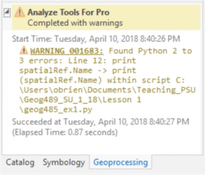
As you can see from the image, we get a warning about the print statement (on line 12) as well as a suggestion of what to change that line to. Those warnings are also written into our output file which will be helpful when we’re trying to modify longer pieces of code (or if you wanted to share the task among many programmers).
1.5.1 Making a Script Tool
Here’s another simple script that finds all cells over 3500 meters in an elevation raster and makes a new raster that codes all those cells as 1. Remaining values in the new raster are coded as 0. By now, you’re probably familiar with this type of “map algebra” operation which is common in site selection and other GIS scenarios.
Just in case you’ve forgotten, the expression Raster(inRaster) tells arcpy that it needs to treat your inRaster variable as a raster dataset so that you can perform map algebra on it. If you didn't do this, the script would treat inRaster as just a literal string of characters (the path) instead of a raster dataset.
# This script uses map algebra to find values in an
#  elevation raster greater than 3500 (meters).

import arcpy
from arcpy.sa import *

# Specify the input raster
inRaster = "C:/Data/Elevation/foxlake"
cutoffElevation = 3500

# Check out the Spatial Analyst extension
arcpy.CheckOutExtension("Spatial")

# Make a map algebra expression and save the resulting raster
outRaster = Raster(inRaster) > cutoffElevation
outRaster.save("C:/Data/Elevation/foxlake_hi_10")

# Check in the Spatial Analyst extension now that you're done
arcpy.CheckInExtension("Spatial")
You can probably easily work out what this script is doing but, just in case, the main points to remember on this script are:
- Notice the lines of code that check out the Spatial Analyst extension before doing any map algebra and check it back in after finishing. Because each line of code takes some time to run, avoid putting unnecessary code between checkout and checkin. This allows others in your organization to use the extension if licenses are limited. The extension automatically gets checked back in when your script ends, thus some of the Esri code examples you will see do not check it in. However, it is a good practice to explicitly check it in, just in case you have some long code that needs to execute afterward, or in case your script crashes and against your intentions "hangs onto" the license.
- inRaster begins as a string, but is then used to create a Raster object once you run Raster(inRaster). A Raster object is a special object used for working with raster datasets in ArcGIS. It's not available in just any Python script: you can use it only if you import the arcpy module at the top of your script.
- cutoffElevation is a number variable that you declare early in your script and then use later on when you build the map algebra expression for your outRaster.
- The expression outRaster = Raster(inRaster) > cutoffElevation is saying, in plain terms, "Make a new raster and call it outRaster. Do this by taking all the cells of the raster dataset at the path of inRaster that are greater than the number assigned to the variable cutoffElevation."
- outRaster is also a Raster object, but you have to call the method outRaster.save() in order to make it permanent on disk. The save() method takes one argument, which is the path to which you want to save.
Copy the code above into a file called Lesson1A.py (or similar as long as it has a .py extension) in spyder or your favorite IDE or text editor and then save it.
We don’t need to do anything to this code to get it to work in Python 3, it will be fine just as it is. Feel free to check it against Analyze Tools for Pro if you like. Your results should say “Analyze Tools for Pro Completed Successfully” with the lack of warnings signifying that the code you supplied is compatible with Python 3.
Next, we'll convert the script to a Tool.
1.5.1.1 Converting the script to a tool
Now, let’s convert this script to a script tool in ArcGIS Pro to familiarize ourselves with the process and we’ll examine the differences between ArcGIS Desktop and ArcGIS Pro when it comes to working with script tools (hint: there aren’t any other than the interface looking slightly different).
We’ll get started by opening ArcGIS Pro. You will be prompted to sign in (use your Penn State ArcGIS Online account which you should already have) and create a project when Pro starts.
Signing in to ArcGIS Pro is an important, new development for running code in Pro as compared to Desktop. As you may be aware, Pro operates with a different licensing structure such that it will regularly "phone home" to Esri's license servers to check that you have a valid license. With Desktop, once you had installed it and set up your license, you could run it for the 12 months the license was valid, online or offline, without any issues. As Pro will regularly check-in with Esri, we need to be mindful that if our code stops working due to an extension not being licensed error or due to a more generic licensing issue, we should check that Pro is still signed in. For nearly everyone, this won't be an issue as you'll generally be using Pro on an Internet connected computer and you won't notice the licensing checks. If you take your computer offline for an extended period, you will need to investigate Esri's offline licensing options.
Projects are Pro’s way of keeping all of your maps, layouts, tasks, data, toolboxes etc. organized. If you’re coming from Desktop, think of it as an MXD with a few more features (such as allowing multiple layouts for your maps).
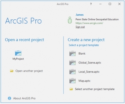
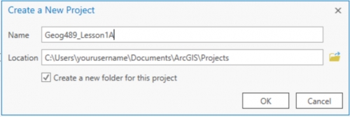
Choose to Create a new project using the Blank template, give it a meaningful name and put it in a folder appropriate for your local machine (things will look slightly different in version 3.0 of Pro: simply click on the Map option under New Project there if you are using that version).
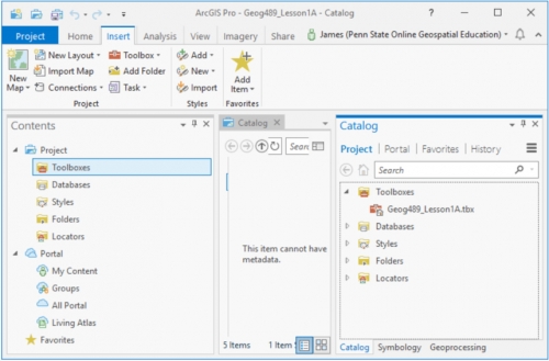
You will then have Pro running with your own toolbox already created. In the figure below, I’ve clicked on the Toolboxes to expand it to show the toolbox which has the same name as my project.
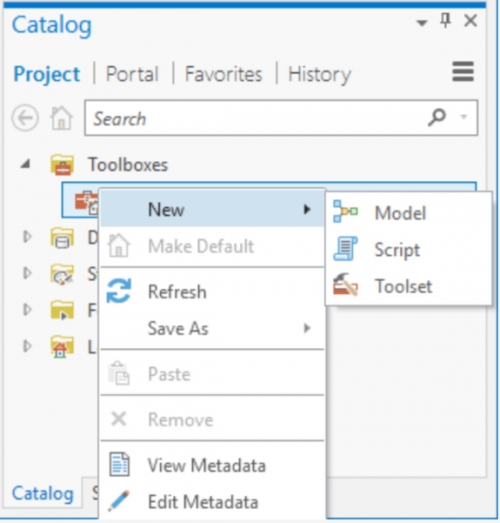
If we right-click on our toolbox we can choose to create a New > Script.
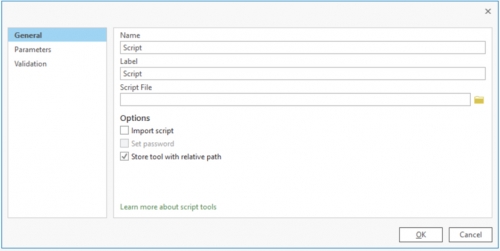
A window will pop up allowing us to enter a name for our script (“Lesson1A”) and a label for our script (“Geog 489 Lesson 1A”), and then we’ll use the file browse icon to locate the script file we saved earlier. In new versions of Pro (2.9 and 3.0), the script file now has to be selected in a new tab called "Execution" located below "Parameters". If your script isn’t showing up in that folder or you get a message that says “Container is empty” press F5 on your keyboard to refresh the view.
We won’t choose to “Import Script” or define any parameters (yet) or investigate validation (yet). When we click OK, we’ll have our script tool created in Pro. We’re not going to run our script tool (yet) as it’s currently expecting to find the foxlake DEM data in C:\data\elevation and write the results back to that folder which is not very convenient. It also has the hardcoded cutoff of 3500 embedded in the code. You can download the FoxLake DEM here.
To make the script more user-friendly, we’re going to make a few changes to allow us to pick the location of the input and output files as well as allow the user to input the cutoff value. Later we’ll also use validation to check whether that cutoff value falls inside the range of values present in the raster and, if not, we’ll change it.
We can edit our script from within Pro, but if we do that it opens in Notepad which isn’t the best environment for coding. You can use Notepad if you like, but I’d suggest opening the script again in your favorite text editor (I like Notepad++) or just using spyder.
If you want, you can change this preferred editor by modifying Pro’s geoprocessing options (see http://pro.arcgis.com/en/pro-app/help/analysis/geoprocessing/basics/geoprocessing-options.htm). To access these options in Pro, click Home -> Options -> Geoprocessing Options. Here you can also choose an option to automatically validate tools and scripts for Pro compatibility (so you don’t need to run the Analyze Tools for Pro manually each time).
We're going to make a few changes to our code now, swapping out the hardcoded paths in lines 8 and 17 and the hardcoded cutoffElevation value in line 9. We’re also setting up an outPath variable in line 10 and setting it to arcpy.env.workspace.
You might recall from GEOG 485 or your other experience with Desktop that the default workspace in Desktop is usually default.gdb in your user path. Pro is smarter than that and sets the default workspace to be the geodatabase of your project. We’ll take advantage of that to put our output raster into our project workspace. Note the difference in the type of parameter we’re using in lines 8 & 9. It’s ok for us to get the path as Text, but we don’t want to get the number in cutoffElevation as Text because we need it to be a number.
To simplify the programming, we’ll specify a different parameter type in Pro and let that be passed through to our script. To make that happen, we’ll use GetParameter instead of GetParameterAsText.
# This script uses map algebra to find values in an
#  elevation raster greater than 3500 (meters).

import arcpy
from arcpy.sa import *

# Specify the input raster
inRaster = arcpy.GetParameterAsText(0)
cutoffElevation = arcpy.GetParameter(1)
outPath = arcpy.env.workspace

# Check out the Spatial Analyst extension
arcpy.CheckOutExtension("Spatial")

# Make a map algebra expression and save the resulting raster
outRaster = Raster(inRaster) > cutoffElevation
outRaster.save(outPath+"/foxlake_hi_10")

# Check in the Spatial Analyst extension now that you're done
arcpy.CheckInExtension("Spatial")
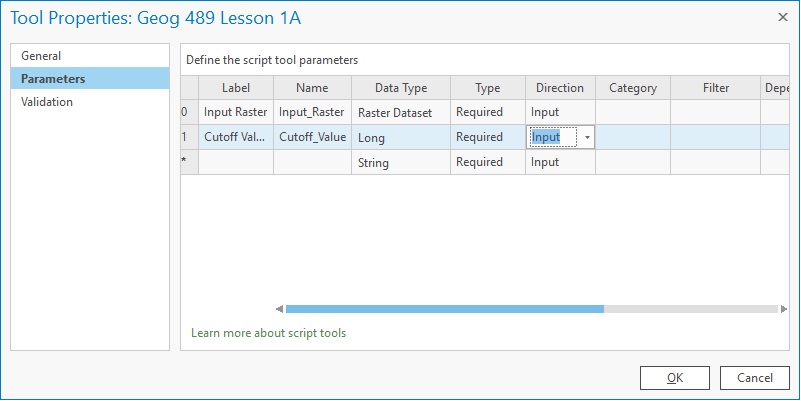
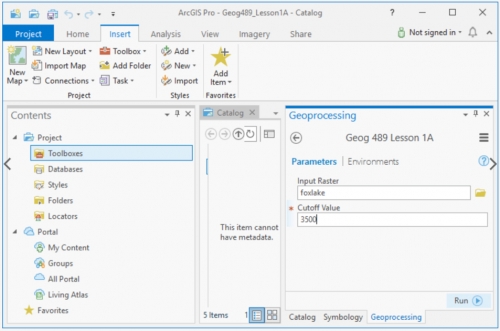
Once you have made those changes, save the file and we’ll go back to our script tool in Pro and update it to use the parameters we’ve just defined. Right click on the script tool within the toolbox and choose Properties and then click Parameters. The first parameter we defined (remember Python counts from 0) was the path to our input raster (inRaster), so let's set that up. Click in the text box under Label and type “Input Raster” and when you click into Name you’ll see that Name is already automatically populated for you. Next, click the Data Type (currently String) and change it to “Raster Dataset” and we’ll leave the other values with their defaults.
Click the next Label text box below your first parameter (currently numbered with a *) and type “Cutoff Value” and change the Data Type to Long (which is a type of number) and we’ll keep the rest of the defaults here too. The final version should look as in the figure below.
Click OK and then we’ll run the tool to test the changes we made by double-clicking it. Use the file icon alongside our Input Raster parameter to navigate to your foxlake raster (which is the FoxLake digital elevation model (DEM) in your Lesson 1 data folder) and then enter 3500 into the cutoff value parameter and click OK to run the tool.
The tool should have executed without errors and placed a raster called foxlake_hi_10 into your project geodatabase.
If it doesn’t work the first time, verify that:
- you have supplied the correct input and output paths;
- your path name contains forward slashes (/) or double backslashes (\\), not single backslashes (\);
- the Spatial Analyst Extension is available. To check this, go Project -> Licensing and check under Esri Extensions;
- you do not have any of the datasets open in ArcGIS;
- the output data does not exist yet. If you want to be able to overwrite the output, you need to add the line "arcpy.env.overwriteOutput = True." This line can be placed immediately after " import arcpy."
1.5.1.2 Adding tool validation code
Now let’s expand on the user friendliness of the tool by using the validator methods to ensure that our cutoff value falls within the minimum and maximum values of our raster (otherwise performing the analysis is a waste of resources).
The purpose of the validation process is to allow us to have some customizable behavior depending on what values we have in our tool parameters. For example, we might want to make sure a value is within a range as in this case (although we could do that within our code as well), or we might want to offer a user different options if they provide a point feature class instead of a polygon feature class, or different options if they select a different type of field (e.g. a string vs. a numeric type).
The Esri help for Tool Validation gives a longer list of uses and also explains the difference between internal validation (what Desktop & Pro do for us already) and the validation that we are going to do here which works in concert with that internal validation.
You will notice in the help that Esri specifically tells us not to do what I’m doing in this example – running geoprocessing tools. The reason for this is they generally take a long time to run. In this case, however, we’re using a very simple tool which gets the minimum & maximum raster values and therefore executes very quickly. We wouldn’t want to run an intersection or a buffer operation for example in the ToolValidator, but for something very small and fast such as this value checking, I would argue that it’s ok to break Esri’s rule. You will probably also note that Esri hints that it’s ok to do this by using Describe to get the properties of a feature class and we’re not really doing anything different except we’re getting the properties of a raster.
So how do we do it? Go back to your tool (either in the Toolbox for your Project, Results, or the Recent Tools section of the Geoprocessing sidebar), right click and choose Properties and then Validation.
You will notice that we have a pre-written, Esri-provided class definition here. We will talk about how class definitions look in Python in Lesson 4 but the comments in this code should give you an idea of what the different parts are for. We’ll populate this template with the lines of code that we need. For now, it is sufficient to understand that different methods (initializeParameters(), updateParameters(), etc.) are defined that will be called by the script tool dialog to perform the operations described in the documentation strings following each line starting with def.
Take the code below and use it to overwrite what is in your ToolValidator:
import arcpy
class ToolValidator(object):
"""Class for validating a tool's parameter values and controlling
the behavior of the tool's dialog."""
def __init__(self):
"""Setup arcpy and the list of tool parameters."""
self.params = arcpy.GetParameterInfo()
def initializeParameters(self):
"""Refine the properties of a tool's parameters. This method is
called when the tool is opened."""
def updateParameters(self):
"""Modify the values and properties of parameters before internal
validation is performed. This method is called whenever a parameter
has been changed."""
def updateMessages(self):
"""Modify the messages created by internal validation for each tool
parameter. This method is called after internal validation."""
## Remove any existing messages
self.params[1].clearMessage()
if self.params[1].value is not None:
## Get the raster path/name from the first [0] parameter as text
inRaster1 = self.params[0].valueAsText
## calculate the minimum value of the raster and store in a variable
elevMINResult = arcpy.GetRasterProperties_management(inRaster1, "MINIMUM")
## calculate the maximum value of the raster and store in a variable
elevMAXResult = arcpy.GetRasterProperties_management(inRaster1, "MAXIMUM")
## convert those values to floating points
elevMin = float(elevMINResult.getOutput(0))
elevMax = float(elevMAXResult.getOutput(0))
## calculate a new cutoff value if the original wasn't suitable but only if the user hasn't specified a value.
if self.params[1].value < elevMin or self.params[1].value > elevMax:
cutoffValue = elevMin + ((elevMax-elevMin)/100*90)
self.params[1].value = cutoffValue
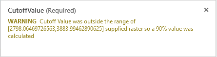
self.params[1].setWarningMessage("Cutoff Value was outside the range of ["+str(elevMin)+","+str(elevMax)+"] supplied raster so a 90% value was calculated")
Our logic here is to take the raster supplied by the user and determine the min and max values so that we can evaluate whether the cutoff value supplied by the user falls within that range. If that is not the case, we're going to do a simple mathematical calculation to find the value 90% of the way between the min and max values and suggest that as a default to the user (by putting it into the parameter). We’ll also display a warning message to the user telling them that the value has been adjusted and why their original value doesn’t work.
As you look over the code, you’ll see that all of the work is being done in the bottom function updateMessages(). This function is called after the updateParameters() and the internal arcpy validation code have been executed. It is mainly intended for modifying the warning or error messages produced by the internal validation code. The reason why we are putting all our validation code here is because we want to produce the warning message and there is no entirely simple way to do this if we already perform the validation and potentially automatic adjustment of the cutoff value in updateParameters() instead. Here is what happens in the updateMessages() function:
We start by cleaning up any previous messages self.params[1].clearMessages() (line 24). Then we check if the user has entered a value into the cutoffValue parameter (self.params[1]) on line 26. If they haven't, we don’t do anything (for efficiency). If the user has entered a value (i.e., the value is not None) then we get the raster name from the first parameter (self.params[0]) and we extract it as text (because we want the content to use as a path) on line 28. Then we’ll call the arcpy GetRasterProperties function twice, once to get the min value (line 30) and again to get the max value (on line 32) of the raster. We’ll then convert those values to floating point numbers (lines 34 & 35).
Once we’ve done that, we do a little bit of checking to see if the value the user supplied is within the range of the raster. If it is not, then we will do some simple math to calculate a value that falls 90% of the way into the range and then update the parameter (self.params[1].value) with the number we calculated (line 40 and 41). Finally, in line 42, we produce the warning message informing the users of the automatic value adjustment.
Now let’s test our Validator. Click OK and return to your script in the Toolbox, Results or Geoprocessing window. Run the script again. Insert the name of the input raster again. If you didn’t make any mistakes entering the code there won’t be a red X by the Input Raster. If you did make a mistake, an error message will be displayed there, showing you the usual arcpy / geoprocessing error message and the line of code that the error is occurring on. If you have to do any debugging, exit the script, return to the Toolbox, right click the script and go back to the Tool Validator and correct the error. Repeat as many times as necessary.
If there were no errors, we should test out our validation by putting a value into our Cutoff Value parameter that we know to be outside the range of our data. If you choose a value < 2798 or > 3884, you should see a yellow warning triangle appear that displays our error message, and you will also note that the value in Cutoff Value has been updated to our 90% value.
We can change the value to one we know works within the range (e.g. 3500), and now the tool should run.
1.6 Performance and how it can be improved
Now that we are back into the groove of writing arcpy code and creating script tools, we want to look at a topic that didn't play a big role in our introductory class, GEOG 485, but that is very important to programming: We want to talk about run-time performance and the related topics of parallelisation and code profiling. These will be the main topics of the next sections and this lesson in general.
We are going to address the question of how we can improve the performance and reliability of our Python code when dealing with more complicated tasks that require a larger number of operations on a greater number of datasets and/or more memory. To do this we’re going to look at both 64-bit processing and multiprocessing. We’re going to start investigating these topics using a simple raster script to process LiDAR data from Penn State’s main campus and surrounding area. In later sections, we will also look at a vector data example using different data sets for Pennsylvania.
The raster data consists of 808 tiles which are all individually zipped, 550MB zipped in total. The individual .zip files can be downloaded from PASDA directly.
Previously PASDA provided access via FTP but unfortunately that ability has been removed. However, we recommend you use a little Python script we put together that uses BeautifulSoup (which we'll look at more in Lesson 2) to download the files. The script will also automatically extract the individual .zip files. For this you have to do the following:
- Download the script from here at github or simply copy & paste the code into a new script file in Spyder (or any other development environment).
- At the beginning of the main function, two folders are specified, the first one for storing the .zip files and the second for storing the extracted raster files. These are currently set to C:\temp and C:\temp\unzipped but you may not have the permissions to write to these folders. We therefore recommend that you edit these variables to have the LiDAR files downloaded and extracted to folders within your Windows user's home directory, e.g. C:\Users\<username>\Documents\489 and C:\Users\<username>\Documents\489\unzipped (assuming that the folder 489 already exist in your Documents folder). The script uses a wildcard on line 66 that tells Python to only download tile files with 227 in the file name, not all of them. This is ok for running the code examples in this lesson but if you want to do test runs with more or all the files, you can also edit this line so that it reads wildcard_pattern = "zip" (because "zip" exists in all the filenames)
- Run the script and you should see the downloaded .zip files and extracted raster files appear in the specified target folders.
Doing any GIS processing with these LiDAR files is definitely a task to be handled by scripting, and any performance benefits we can gain when we’re processing that many tiles will be worthwhile. The question you might be asking is why don’t we just join all of the tiles together and process them at once - we’d run out of memory very fast and if something goes wrong we need to start over. Processing small tiles we can do one (or a few) at a time using less memory and if one tile fails we still have all of the others and just need to restart that tile.
Below is our simple raster script which gets our list of tiles and then for every tile in the list we fill the DEM, create a flow direction and flow accumulation raster to then derive a stream raster (to determine where the water might flow), and lastly we convert the stream raster to polygon or polyline feature classes. This is a simplified version of the sort of analysis you might undertake to prepare data prior to performing a flood study. The code we are writing here will work in both Desktop and Pro as long as you have the Spatial Analyst extension installed, authorized and enabled (it is this last step that generally causes errors). I’ve restricted the processing to a subset of those tiles for testing and performance reasons using only tiles with 227 in the name but more tiles can be included by modifying the wild card list in line 19.
If you used the download script above, you already have the downloaded raster files ready. You can move them to a new folder or keep them where they are. In any case, you will need to make sure that the workspace in the script below points to the folder containing the extracted raster files (line 9). If you obtained the raster files in some other way, you may have to unzip them to a folder first.
Let’s look over the code now. You will notice that the version below is for Python 3 (the print function gives it away) but it will work in both Python 2 and 3 without changes.
# Setup _very_ simple timing.
import time
process_start_time = time.time()

import arcpy
from arcpy.sa import *

arcpy.env.overwriteOutput = True
arcpy.env.workspace = r'C:\489\PSU_LiDAR'

## If our rasters aren't in our filter list then drop them from our list.
def filter_list(fileList,filterList):
    return[i for i in fileList if any(j in i for j in filterList)]

# Ordinarily we would want all of the rasters I'm filtering by a small set for testing & efficiency
# I did this by manually looking up the tile index for the LiDAR and determining an area of interest
# tiles ending in 227, 228, 230, 231, 232, 233, 235, 236

wildCardList = set(['227']) ##,'228','230','231','232','233','235','236'])
# Get a list of rasters in my folder
rasters = arcpy.ListRasters("*")
new_rasters = filter_list(rasters,wildCardList)

# for all of our rasters
for raster in new_rasters:
    raster_start_time = time.time()
    # Now that we have our list of rasters
    ## Note also for performance we're not saving any of the intermediate rasters - they will exist only in memory
    ## Fill the DEM to remove any sinks
    try:
        FilledRaster = Fill(raster)
        ## Calculate the Flow Direction (how water runs across the surface)
        FlowDirRaster = FlowDirection(FilledRaster)
        ## Calculate the Flow Accumulation (where the water accumulates in the surface)
        FlowAccRaster = FlowAccumulation(FlowDirRaster)
        ## Convert the Flow Accumulation to a Stream Network
        ## We're setting an arbitray threshold of 100 cells flowing into another cell to set it as part of our stream
        ## http://pro.arcgis.com/en/pro-app/tool-reference/spatial-analyst/identifying-stream-networks.htm
        Streams = Con(FlowAccRaster,1,"","Value > 100")
        ## Convert the Raster Stream network to a feature class
        output_Polyline = raster.replace(".img",".shp")
        arcpy.CheckOutExtension("Spatial")
        arcpy.sa.StreamToFeature(Streams,FlowDirRaster,output_Polyline)
        arcpy.CheckInExtension("Spatial")
    except:
        print ("Errors occured")
        print (arcpy.GetMessages())
        arcpy.AddMessage ("Errors occurred")
        arcpy.AddMessage(arcpy.GetMessages())

# Output how long the whole process took.
arcpy.AddMessage("--- %s seconds ---" % (time.time() - process_start_time))
print ("--- %s seconds ---" % (time.time() - process_start_time))
We have set up some very simple timing functionality in this script using the time() function defined in the module time of the Python standard library. The function gives you the current time and, by calling it at the beginning and end of the program and then taking the difference in the very last line of the script, we get an idea of the runtime of the script.
Later in the lesson, we will go into more detail about properly profiling code where we will examine the performance of a whole program as well as individual instructions. For now, we just want an estimate of the execution time. Of course, it’s not going to be very precise as it will depend on what else you’re doing on your PC at the same time and we would need to run a number of iterations to remove any inconsistencies (such as the delay when arcpy loads for the first time etc.). On my PC that code runs in around 40 seconds. Your results will vary depending on many factors related to the performance of your PC (we'll review some of them in the Speed Limiters section) but you should test out the code to get an idea of the baseline performance of the algorithm on your PC.
In lines 12 and 13, we have a simple function to filter our list of rasters to just those we want to work with (centered on the PSU campus). This function might look a little different to what you have seen before - that's because we're using list comprehension which we'll examine in more detail in Lesson 2. So don't worry about understanding how exactly this works at the moment. It basically says to return a list with only those file names from the original list that contain one of the numbers in the wild card list.
We set up some environment variables, our wildcard list (used by our function for filtering) at line 19 - where you will notice I have commented out some of the list for speed during testing, and then we get our list of rasters, filter it and for those rasters left and we iterate through them with the central for-loop in line 25 performing our spatial analysis tasks mentioned earlier. There is some basic error checking wrapped around the tasks (which is also reporting running times if anything goes wrong) and then lastly there is a message and print function with the total time. I’ve included both print and AddMessage just in case you wanted to test the code as a script tool in ArcGIS.
Feel free to run the script now and see what total computation time you get from the print statement in the last line of the code. We‘re going to demonstrate some very simple performance evaluation of the different versions of ArcGIS (32 bit Desktop, 64 bit Desktop, Pro and arcpy Multiprocessing) using this code. Before we do that though it is important to understand the differences between each of them. You do not have to run this testing yourself; we’re mainly providing it as some background. You are welcome to experiment with it, but please do not do that to the detriment of your project.
Once we’ve examined the theory of 64-bit processing and parallelisation and worked through a simple example using the Hi-ho Cherry-O game from GEOG 485, we’ll come back to the raster example above and convert it to running in parallel using the Python multiprocessing package instead of sequentially and we will further look at an example of multiprocessing using vector data.
1.6.1 32-bit vs. 64-bit processing
32-bit software or hardware can only directly represent and operate with numbers up to 2^32 and, hence, can only address up to a maximum of 4GB of memory (that is 2^32 = 4294967296 bytes). If the file system of your operating system is limited to 32-bit integers as well, this also means you cannot have any single file larger than 4GB either in memory or on disk (you can still page or chain larger files together though).
64-bit architectures don’t have this limit. Instead you can access up to 16 terabytes of memory and this is actually only the limit of current chip architectures which "only" use 44 bits which will change over time as software and hardware architectures evolve. Technically with a 64-bit architecture you could access 16 Exabytes of memory (2^64) and while not wanting to paraphrase Bill Gates, that is probably more than we’ll need for the foreseeable future.
There most likely won't be any innate performance benefits to be gained by moving from 32-bit and 64-bit unless you need that extra memory. While in principle, you can move larger amounts of data per time between memory and CPU with 64-bit, this typically doesn't result in significantly improved execution times because of caching and other optimization techniques used by modern CPUs. However if we start using programming models where we run many tasks at once, you might want more than 4GB allocated to those processes. For example if you had 8 tasks that all needed 500MB of RAM each – that’s very close to the 4GB limit in total (500MB * 8 = 4000MB). If you had a machine with more processors (e.g. 64) you would very easily hit the 32-bit 4GB limit as you would only be able to allocate 62.5MB of RAM per processor from your code.
Even with hardware architectures and operating systems mainly being 64-bit these days, a lot of software still is only available as 32-bit versions. 64-bit operating systems are designed to be backwards compatible with 32-bit applications, and if there is no real expected benefit for a particular software, the developer of the software may just as well decide to stick with 32-bit and avoid the efforts and costs that it would take to make the change to 64-bit or even support multiple versions of the software. ArcGIS Desktop is an example of a software that is only available as 32-bit and this is (most likely) not going to change anymore since ArcGIS Pro, which is 64-bit, fills that role. However, Esri also provides a 64-bit geoprocessing extension for ArcGIS Desktop which will be further described in the next section. However, this section is considered optional. You may read through it and learn how it can be set up and about what performance gain can be achieved using it or you may skip most of it and just have a look at the table with the computation time comparison at the very end of the section. But we strongly recommend that you do not try to install 64-bit geoprocessing and perform the steps yourself before you have worked through the rest of lesson and the homework assignment.
1.6.2 Optional complementary materials: 64-bit background geoprocessing in ArcGIS Desktop
This section is provided for interest only - as it only applies to ArcGIS Desktop - not Pro (which is natively 64 bit). It is recommended that you only read/skim through the section and check out the computation time comparison at the end without performing the described steps yourself and then loop back to it at the end of the lesson if you have free time and are interested in exploring 64-bit Background Geoprocessing in ArcGIS Desktop.
A number of versions ago (since Server 10.1), Esri added support for 64-bit arcpy. Esri also introduced 64-bit geoprocessing using the 64-bit Background Geoprocessing patch which was part of 10.1 Service Pack 1 as an option in ArcGIS Desktop (Pro is entirely 64-bit) to work around these memory issues for large geoprocessing tasks. Not all tools support 64-bit geoprocessing within Desktop and there are some tricks to getting it installed so you can access it in Desktop. There is also a 64-bit arcpy geoprocessing library so you can run your code (any code) from the command line. Background Geoprocessing (64-bit) is still available as a separate installation on top of ArcGIS (see this ArcMap/Background Geoprocessing (64-bit) page) and we’ve provided a link for students to obtain it within Canvas. You'll find this link on the "64-bit Geoprocessing downloads for ArcGIS (optional)" page under Lesson 1 in Canvas.
As Esri hint in their documentation, 64-bit processing within ArcGIS Desktop requires that the tool run in the background. This is because it is running using a separate set of tools which are detached from the Desktop application (which is 32-bit). Personally, I rarely use Background Geoprocessing but I do make use of the 64-bit version of Python that it installs to run a lot of my scripts in 64-bit mode from the command line.
If you’ve typically run your code in the past from within an IDE (such as PythonWin, IDLE or spyder) or from within ArcGIS you might not be aware that you can also run that code from the command line by calling Python directly.
For ArcGIS Desktop you can start a regular command prompt and, using the standard Windows commands, change to that path where your Python script is located. Usually when you open a command window, it will start in your home folder (e.g. c:\users\yourname). We could dedicate an entire class to operating system commands but Microsoft has a good resource at this Windows Commands page for those who are interested.
We just need a couple of the commands listed there :
- cd : change directory. We use this to move around our folders. Full help at this Commands/cd page.
- dir : list the files and folders in my directory. Full help at this Commands/dir page.
We’ll change the directory to where our code from section 1.6 is (e.g. mine is c:\wcgis\geog489\lesson1) and see how to run the script using the command line versions of 32-bit and 64-bit Python.
cd c:\wcgis\geog489\lesson1
If you downloaded and installed the 64-bit Background Geoprocessing from above you will have both 32-bit and 64-bit Python installed. We’ll use the 32-bit Python first which should be located at c:\python27\arcgis10.6\python.exe (substitute 10.6 by whichever version of ArcGIS you have installed).
There’s a neat little feature built into the command line where you can use the TAB key to autocomplete paths so you could start typing c:\python27\a and then hit TAB and you should see the path cycling through the various ArcGIS folders.
We’ll run our code using:
C:\python27\ArcGIS10.6\python.exe myScriptName.py
Where myScriptName.py is whatever you saved the code from section 1.6 as. You will now see the code run in the command window and pop up all of the same messages you would have seen if you had run it from an IDE (but not the AddMessages messages as they are only interpreted by ArcGIS).
To run the code against the 64-bit version of Python the command is almost identical except that you’ll use the x64 version of Python that has been installed by Background Geoprocessing. In my case that means the command is:
C:\python27\ArcGISx6410.5\python.exe myScriptName.py
Once your script finishes you’ll have a few time stamp values. Running that code from Section 1.6 through the 32-bit and 64-bit versions a few times we have some sample results below. The first runs of each are understandably slower as arcpy is imported for the first time. You have probably witnessed this behavior yourself as your code takes longer the very first time it runs.
| 32-bit Desktop | 64-bit Desktop | 64-bit Pro |
|---|---|---|
| 149 seconds | 107 seconds | 109 seconds |
| 119 seconds | 73 seconds | 144 seconds |
| 91 seconds | 90 seconds | 111 seconds |
| 85 seconds | 73 seconds | |
| 93 seconds | 75 seconds |
We can see a couple of things with these results – they are a little inconsistent depending on what else my PC was doing at the time the code was running and, if you are looking at individual executions of the code, it is difficult to see which pieces of the code are slower or faster from time to time. This is the problem that we will solve later in the lesson when we look at profiling code where we examine how long each line of code takes to run.
1.6.3 Parallel processing
You have probably noticed if you have a relatively modern PC (anything from the last several years) that when you open Windows Task Manager (from the bottom of the list when you press CTRL-ALT-DEL) and you click the Performance tab and right click on the CPU graph and choose Change Graph to -> Logical Processors you have a number of processors (or cores) within your PC. These are actually “logical processors“ within your main processor but they function as though they were individual processors – and we’ll just refer to them as processors here for simplicity.
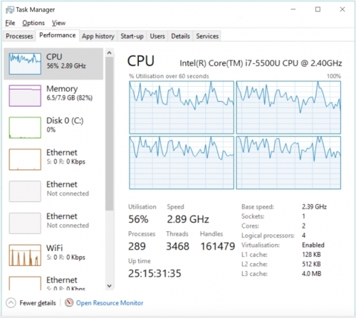
Now because we have multiple processors, we can run multiple tasks in parallel at the same time instead of one at a time. There are two ways that we can run tasks at the same time – multithreaded and multiprocessing. We’ll look at the differences in each in the following but it’s important to know that arcpy doesn’t support multithreading but it does support multiprocessing. In addition, there is a third form of parallelisation called distributed computing, which involves distributing the task over multiple computers, that we will also briefly talk about.
1.6.3.1 Multithreading
Multithreading is based on the notion of "threads" for a number of tasks that are executed within the same memory space. The advantage of this is that because the memory is shared between the threads they can share information. This results in a much lower memory overhead because information doesn’t need to be duplicated between threads. The basic logic is that a single thread starts off a task and then multiple threads are spawned to undertake sub-tasks. At the conclusion of those sub-tasks all of the results are joined back together again. Those threads might run across multiple processors or all on the same one depending on how the operating system (e.g. Windows) chooses to prioritize the resources of your computer. In the example of the PC above which has 4 processors, a single-threaded program would only run on one processor while a multi-threaded program would run across all of them (or as many as necessary).
1.6.3.2 Multiprocessing
Multiprocessing achieves broadly the same goal as multi-threading which is to split the workload across all of the available processors in a PC. The difference is that multiprocessing tasks cannot communicate directly with each other as they each receive their own allocation of memory. That means there is a performance penalty as information that the processes need must be stored in each one. In the case of Python a new copy of python.exe (referred to as an instance) is created for each process that you launch with multiprocessing. The tasks to run in multiprocessing are usually organized into a pool of workers which is given a list of the tasks to be completed. The multiprocessing library will assign each task to a worker (which is usually a processor on your PC) and then once a worker completes a task the next one from the list will be assigned to that worker. That process is repeated across all of the workers so that as each finishes a task a new one will be assigned to them until there are no more tasks left to complete.
You might have heard of the MapReduce framework which underpins the Hadoop parallel processing approach. The use of the term map might be confusing to us as GIS folks as it has nothing to do with our normal concept of maps for displaying geographical information. Instead in this instance map means to take a function (as in a programming function) and apply it once to every item in a list (e.g. our list of rasters from the earlier example).
The reduce part of the name is similar as we apply a function to a list and combine the results of our function into a single result (e.g. a list from 1 – 10,000 which is our number of Hi-ho Cherry-O games and we want the number of turns for each game).
The two elements map and reduce work harmoniously to solve our parallel problems. The map part takes our one large task (which we have broken down into a number of smaller tasks and put into a list) and applies whatever function we give it to the list (one item in the list at a time) on each processor (which is called a worker). Once we have a result, that result is collected by the reduce part from each of the workers and brought back to the calling function. There is a more technical explanation in the Python documentation.
Multiprocessing in Python
At around the same time that Esri introduced 64-bit processing, they also introduced multiprocessing to some of the tools within ArcGIS Desktop (mostly raster based tools in the first iteration) and also added multiprocessor support to the arcpy library.
Multiprocessing has been available in Python for some time and it’s a reasonably complicated concept so we will do our best to simplify it here. We’ll also provide a list of resources at the end of this section for you to continue exploring if you are interested. The multiprocessing package of Python is part of the standard library and has been available since around Python 2.6. The multiprocessing library is required if you want to implement multiprocessing and we import it into our code just like any other package using:
import multiprocessing
Using multiprocessing isn’t as simple as switching from 32-bit to 64-bit as we did above. It does require some careful thought about which processes we can run in parallel and which need to run sequentially. There are also issues about file sharing and file locking, performance penalties where sometimes multiprocessing is slower due to the time taken to setup and remove the multiprocessing pool, and some tasks that do not support multiprocessing. We’ll cover all of these issues in the following sections and then we’ll convert our simple, sequential raster processing example into a multiprocessing one to demonstrate all of these concepts.
1.6.3.3 Distributed processing
Distributed processing is a type of parallel processing that instead of (just) using each processor in a single machine will use all of the processors across multiple machines. Of course, this requires that you have multiple machines to run your code on but with the rise of cloud computing architectures from providers such as Amazon, Google, and Microsoft this is getting more widespread and more affordable. We won’t cover the specifics of how to implement distributed processing in this class but we have provided a few links if you want to explore the theory in more detail.
In a nutshell what we are doing with distributed processing is taking our idea of multiprocessing on a single machine and instead of using the 4 or however many processors we might have available, we're accessing a number of machines over the internet and utilizing the processors in all of them. Hadoop is one method of achieving this and others include Amazon's Elastic Map Reduce, MongoDB and Cassandra. GEOG 865 has cloud computing as its main topic, so if you are interested in this, you may want to check it out.
1.6.4 Speed limiters
With all of these approaches to speeding up our code, what are the elements which will cause bottlenecks and slow us down?
Well, there are a few – these include the time to set up each of the processes for multiprocessing. Remember earlier we mentioned that because each process doesn’t share memory it needs a copy of the data to use. This will need to be copied to a memory location. Also as each process runs its own Python.exe instance, it needs to be launched and arcpy needs to be imported for each instance (although fortunately, multiprocessing takes care of this for us). Still, all of that takes time to start so our code won’t appear to do much at first while it is doing this housekeeping - and if we're not starting a lot of processes then we won't see enough of a speed up in processing to make up for those start-up time costs.
Other things that can slow us down are the speed of our RAM. Access times for RAM used to be measured in nanoseconds but now are measured in megahertz (MHz). The method of calculating the speed isn’t especially important but if you’re moving large files around in RAM or performing calculations that require getting a number out of RAM, adding, subtracting, multiplying, etc. and then putting the result into another location in RAM and you’re doing that millions of times very, very small delays will quickly add up to seconds or minutes. Another speedbump is running out of RAM. While we can allocate more than 4GB per process using 64-bit programming, if we don’t have enough RAM to complete all of the tasks that we might launch then our operating system will start swapping between RAM (which is fast) and our hard disk (which isn’t – even if it’s one of the solid state types – SSDs).
Speaking of hard disks, it’s very likely that we’re loading and saving data to them and as our disks are slower than our RAM and our processors, that is going to cause a delay. The less we need to load and save data the better, so good multiprocessing practice is to keep as much data as possible in RAM (see the caveat above about running out of RAM). The speed of disks is governed by a couple of factors; the speed that the motor spins (unless it is an SSD), seek time and the amount of cache that the disk has. Here is how these elements all work together to speed up (or slow down) your code. The hard disk receives a request for data from the operating system, which it then goes looking for. This is the seek time referring to how long it takes the disk to position the read head over the segment of disk the data is located on, which is a function of motor speed as well. Then once the file is found, it needs to be loaded into memory – cache - and then this is sent through to the process that needed the data. When data is written back to your disk, the reverse process takes place. The cache is filled (as memory is faster than disks ) and then the cache is written to the disk. If the file is larger than the cache, the cache gets topped up as it starts to empty until the file is written. A slow spinning hard disk motor or a small amount of cache can both slow down this process.
It’s also possible that we’re loading data from across a network connection (e.g. from a database or remotely stored files) and that will also be slow due to network latency – the time it takes to get to and from the other device on the network with the request and the result.
We can also be slowed down by inefficient code, for example, using too many loops or an inefficient if / else / elif statement that we evaluate too many times or using a mathematical function that is slower than its alternatives. We'll examine these sorts of coding bottlenecks - or at least how to identify them when we look at code profiling later in the lesson.
1.6.5 First steps with Multiprocessing
From the brief description in the previous section, you might have realized that there are generally two broad types of tasks – those that are input/output (I/O) heavy which require a lot of data to be read, written or otherwise moved around; and those that are CPU (or processor) heavy that require a lot of calculations to be done. Because getting data is the slowest part of our operation, I/O heavy tasks do not demonstrate the same improvement in performance from multiprocessing as CPU heavy tasks. The more work there is to do for the CPU the greater the benefit in splitting that workload among a range of processors so that they can share the load.
The other thing that can slow us down is outputting to the screen – although this isn’t really an issue in multiprocessing because printing to our output window can get messy. Think about two print statements executing at exactly the same time – you’re likely to get the content of both intermingled, leading to a very difficult to understand message. Even so, updating the screen with print statements is a slow task.
Don’t believe me? Try this sample piece of code that sums the numbers from 0-100.
# Setup _very_ simple timing.
import time
start_time = time.time()

sum = 0
for i in range(0,100):
    sum += i
    print(sum)

# Output how long the process took.
print ("--- %s seconds ---" % (time.time() - start_time))
If I run it with the print function in the loop the code takes 0.049 seconds to run on my PC. If I comment that print function out, the code runs in 0.0009 seconds.
4278
4371
4465
4560
4656
4753
4851
4950
--- 0.04900026321411133 seconds ---

runfile('C:/Users/jao160/Documents/Teaching_PSU/Geog489_SU_21/Lesson 1/untitled1.py', wdir='C:/Users/jao160/Documents/Teaching_PSU/Geog489_SU_21/Lesson 1')
--- 0.0009996891021728516 seconds ---
In Penn State's GEOG 485 course, we simulated 10,000 runs of the children's game Cherry-O to determine the average number of turns it takes. If we printed out the results, the code took a minute or more to run. If we skipped all but the final print statement the code ran in less than a second. We’ll revisit that Cherry-O example as we experiment with moving code from the single processor paradigm to multiprocessor. We’ll start with it as a simple, non arcpy example and then move on to two arcpy examples – one raster (our raster calculation example from before) and one vector.
Since you most likely did not take GEOG 485, you may want to have a quick look at the description.
Following is the original Cherry-O code.
# Simulates 10K game of Hi Ho! Cherry-O
# Setup _very_ simple timing.
import time

start_time = time.time()
import random

spinnerChoices = [-1, -2, -3, -4, 2, 2, 10]
turns = 0
totalTurns = 0
cherriesOnTree = 10
games = 0

while games < 10001:
    # Take a turn as long as you have more than 0 cherries
    cherriesOnTree = 10
    turns = 0
    while cherriesOnTree > 0:
        # Spin the spinner
        spinIndex = random.randrange(0, 7)
        spinResult = spinnerChoices[spinIndex]
        # Print the spin result
        # print ("You spun " + str(spinResult) + ".")
        # Add or remove cherries based on the result
        cherriesOnTree += spinResult

        # Make sure the number of cherries is between 0 and 10
        if cherriesOnTree > 10:
            cherriesOnTree = 10
        elif cherriesOnTree < 0:
            cherriesOnTree = 0
            # Print the number of cherries on the tree
        # print ("You have " + str(cherriesOnTree) + " cherries on your tree.")
        turns += 1
    # Print the number of turns it took to win the game
    # print ("It took you " + str(turns) + " turns to win the game.")
    games += 1
    totalTurns += turns
print("totalTurns " + str(float(totalTurns) / games))
# lastline = raw_input(">")
# Output how long the process took.
print("--- %s seconds ---" % (time.time() - start_time))
We've added in our very simple timing from earlier and this example runs for me in about 1/3 of a second (without the intermediate print functions). That is reasonably fast and you might think we won't see a significant improvement from modifying the code to use multiprocessor mode but let's experiment.
The Cherry-O task is a good example of a CPU bound task; we’re limited only by the calculation speed of our random numbers, as there is no I/O being performed. It is also an embarrassingly parallel task as none of the 10,000 runs of the game are dependent on each other. All we need to know is the average number of turns; there is no need to share any other information. Our logic here could be to have a function (Cherry-O) which plays the game and returns to our calling function the number of turns. We can add that value returned to a variable in the calling function and when we’re done divide by the number of games (e.g. 10,000) and we’ll have our average.
1.6.5.1 Converting from sequential to multiprocessing
So with that in mind, let us examine how we can convert a simple program like Cherry-O from sequential to multiprocessing.
There are a couple of basic steps we need to add to our code in order to support multiprocessing. The first is that our code needs to import multiprocessing which is a Python library which as you will have guessed from the name enables multiprocessing support. We’ll add that as the first line of our code.
The second thing our code needs to have is a __main__ method defined. We’ll add that into our code at the very bottom with:
if __name__ == '__main__':
        mp_handler()
With this, we make sure that the code in the body of the if-statement is only executed for the main process we start by running our script file in Python, not the subprocesses we will create when using multiprocessing, which also are loading this file. Otherwise, this would result in an infinite creation of subprocesses, subsubprocesses, and so on. Next, we need to have that mp_handler() function we are calling defined. This is the function that will set up our pool of processors and also assign (map) each of our tasks onto a worker (usually a processor) in that pool.
Our mp_handler() function is very simple. It has two main lines of code based on the multiprocessing module:
The first instantiates a pool with a number of workers (usually our number of processors or a number slightly less than our number of processors). There’s a function to determine how many processors we have, multiprocessing.cpu_count(), so that our code can take full advantage of whichever machine it is running on. That first line is:
with multiprocessing.Pool(multiprocessing.cpu_count()) as myPool:
   ... # code for setting up the pool of jobs
You have probably already seen this notation from working with arcpy cursors. This with ... as ... statement creates an object of the Pool class defined in the multiprocessing module and assigns it to variable myPool. The parameter given to it is the number of processors on my machine (which is the value that multiprocessing.cpu_count() is returning), so here we are making sure that all processor cores will be used. All code that uses the variable myPool (e.g., for setting up the pool of multiprocessing jobs) now needs to be indented relative to the "with" and the construct makes sure that everything is cleaned up afterwards. The same could be achieved with the following lines of code:
myPool = multiprocessing.Pool(multiprocessing.cpu_count())
... # code for setting up the pool of jobs
myPool.close()
myPool.join()
Here the Pool variable is created without the with ... as ... statement. As a result, the statements in the last two lines are needed for telling Python that we are done adding jobs to the pool and for cleaning up all sub-processes when we are done to free up resources. We prefer to use the version using the with ... as ... construct in this course.
The next line that we need in our code after the with ... as ... line is for adding tasks (also called jobs) to that pool:
res = myPool.map(cherryO, range(10000))
What we have here is the name of another function, cherryO(), which is going to be doing the work of running a single game and returning the number of turns as the result. The second parameter given to map() contains the parameters that should be given to the calls of thecherryO() function as a simple list. So this is how we are passing data to process to the worker function in a multiprocessing application. In this case, the worker function cherryO() does not really need any input data to work with. What we are providing is simply the number of the game this call of the function is for, so we use the range from 0-9,999 for this. That means we will have to introduce a parameter into the definiton of the cherryO() function for playing a single game. While the function will not make any use of this parameter, the number of elements in the list (10000 in this case) will determine how many timescherryO() will be run in our multiprocessing pool and, hence, how many games will be played to determine the average number of turns. In the final version, we will replace the hard-coded number by a variable called numGames. Later in this part of the lesson, we will show you how you can use a different function called starmap(...) instead of map(...) that works for worker functions that do take more than one argument so that we can pass different parameters to it.
Python will now run the pool of calls of the cherryO() worker function by distributing them over the number of cores that we provided when creating the Pool object. The returned results, so the number of turns for each game played, will be collected in a single list and we store this list in variable res. We’ll average those turns per game to get an average using the Python library statistics and the function mean().
To prepare for the multiprocessing version, we’ll take our Cherry-O code from before and make a couple of small changes. We’ll define function cherryO() around this code (taking the game number as parameter as explained above) and we’ll remove the while loop that currently executes the code 10,000 times (our map range above will take care of that) and we’ll therefore need to “dedent“ the code.
Here’s what our revised function will look like :
def cherryO(game):
    spinnerChoices = [-1, -2, -3, -4, 2, 2, 10]
    turns = 0
    cherriesOnTree = 10

    # Take a turn as long as you have more than 0 cherries


    while cherriesOnTree > 0:
        # Spin the spinner
        spinIndex = random.randrange(0, 7)
        spinResult = spinnerChoices[spinIndex]
        # Print the spin result
        #print ("You spun " + str(spinResult) + ".")
        # Add or remove cherries based on the result
        cherriesOnTree += spinResult
        # Make sure the number of cherries is between 0 and 10
        if cherriesOnTree > 10:
            cherriesOnTree = 10
        elif cherriesOnTree < 0:
            cherriesOnTree = 0
        # Print the number of cherries on the tree
        #print ("You have " + str(cherriesOnTree) + " cherries on your tree.")
        turns += 1
    # return the number of turns it took to win the game
    return(turns)
1.6.5.2 Putting it all together
Now lets put it all together. We’ve made a couple of other changes to our code to define a variable at the very top called numGames = 10000 to define the size of our range.
# Simulates 10K game of Hi Ho! Cherry-O
# Setup _very_ simple timing.
import time
start_time = time.time()
import multiprocessing
from statistics import mean
import random
numGames = 10000

def cherryO(game):
    spinnerChoices = [-1, -2, -3, -4, 2, 2, 10]
    turns = 0
    cherriesOnTree = 10

    # Take a turn as long as you have more than 0 cherries


    while cherriesOnTree > 0:
        # Spin the spinner
        spinIndex = random.randrange(0, 7)
        spinResult = spinnerChoices[spinIndex]
        # Print the spin result
        #print ("You spun " + str(spinResult) + ".")
        # Add or remove cherries based on the result
        cherriesOnTree += spinResult
        # Make sure the number of cherries is between 0 and 10
        if cherriesOnTree > 10:
            cherriesOnTree = 10
        elif cherriesOnTree < 0:
            cherriesOnTree = 0
        # Print the number of cherries on the tree
        #print ("You have " + str(cherriesOnTree) + " cherries on your tree.")
        turns += 1
    # return the number of turns it took to win the game
    return(turns)

def mp_handler():
    with multiprocessing.Pool(multiprocessing.cpu_count()) as myPool:
       ## The Map function part of the MapReduce is on the right of the = and the Reduce part on the left where we are aggregating the results to a list.
       turns = myPool.map(cherryO,range(numGames))
    # Uncomment this line to print out the list of total turns (but note this will slow down your code's execution)
    #print(turns)
    # Use the statistics library function mean() to calculate the mean of turns
    print(mean(turns))

if __name__ == '__main__':
    mp_handler()
    # Output how long the process took.
    print ("--- %s seconds ---" % (time.time() - start_time))
You will also see that we have the list of results returned on the left side of the = before our map function (line 40). We’re taking all of the returned results and putting them into a list called turns (feel free to add a print or type statement here to check that it's a list). Once all of the workers have finished playing the games, we will use the Python library statistics function mean, which we imported at the very top of our code (right after multiprocessing) to calculate the mean of our list in variable turns. The call to mean() will act as our reduce as it takes our list and returns the single value that we're really interested in.
When you have finished writing the code in spyder, you can run it. However, it is important to know that there are some well-documented problems with running multiprocessing code directly in spyder. You may only experience these issues with the more complicated arcpy based examples in Section 1.6.6 but we recommend that you run all multiprocessing examples from the command line rather than inside spyder.
The Windows command line and its commands have already been explained in Section 1.6.2 but since this was an optional section, we are repeating the explanation here: Use the shortcut called "Python command prompt" that can be found within the ArcGIS program group on the start menu. This will open a command window running within the Pro conda environment indicating that this is Python 3 (py3). You actually may have several shortcuts with rather similar sounding names, e.g. if you have both ArcGIS Pro and ArcGIS Desktop installed, and it is important that you pick the right one from ArcGIS Pro that mentions Python 3. The prompt will tell you that you are in the folder C:\Users\<username>\AppData\Local\ESRI\conda\envs\arcgispro-py3-clone\ or C:\Program Files\ArcGIS\Pro\bin\Python\envs\arcgispro-py3\ depending on your version of ArcGIS Pro.
We could dedicate an entire class to operating system commands that you can use in the command window but Microsoft has a good resource at this Windows Commands page for those who are interested.
We just need a couple of the commands listed there :
- cd : change directory. We use this to move around our folders. Full help at this Commands/cd page.
- dir : list the files and folders in my directory. Full help at this Commands/dir page.
We’ll change the directory to where we saved the code from above (e.g. mine is in c:\489\lesson1) with the following command:
cd c:\489\lesson1
Before you run the code for the first time, we suggest you change the number of games to a much smaller number (e.g. 5 or 10) just to check everything is working fine so you don’t spawn 10,000 Python instances that you need to kill off. In the event that something does go horribly wrong with your multiprocessing code, see the information about the Windows taskkill command below. To now run the Cherry-O script (which we saved under the name cherry-o.py) in the command window, we use the command:
python cherry-o.py
You should now get the output from the different print statements, in particular the average number of turns and the time it took to run the script. If everything went ok, set the number of games back to 10000 and run the script again.
It is useful to know that there is a Windows command that can kill off all of your Python processes quickly and easily. Imagine having to open Task Manager and manually kill them off, answer a prompt and then move to the next one! The easiest way to access the command is by pressing your Windows key, typing taskkill /im python.exe and hitting Enter which will kill off every task called python.exe. It’s important to only use this when absolutely necessary as it will usually also stop your IDE from running and any other Python processes that are legitimately running in the background. The full help for taskkill is at the Microsoft Windows IT Pro Center taskkill page.
Look closely at the images below, which show a four processor PC running the sequential and multiprocessing versions of the Cherry-O code. In the sequential version, you’ll see that the CPU usage is relatively low (around 50%) and there are two instances of Python running (one for the code and (at least) one for spyder).
In the multiprocessing version, the code was run from the command line instead (which is why it’s sitting within a Windows Command Processor task) and you can see the CPU usage is pegged at 100% as all of the processors are working as hard as they can and there are five instances of Python running.
This might seem odd as there are only four processors, so what is that extra instance doing? Four of the Python instances, the ones all working hard, are the workers, the fifth one that isn’t working hard is the master process which launched the workers – it is waiting for the results to come back from the workers. There isn’t another Python instance for spyder because I ran the code from the command prompt – therefore spyder wasn’t running. We'll cover running code from the command prompt in the Profiling section.
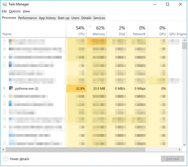
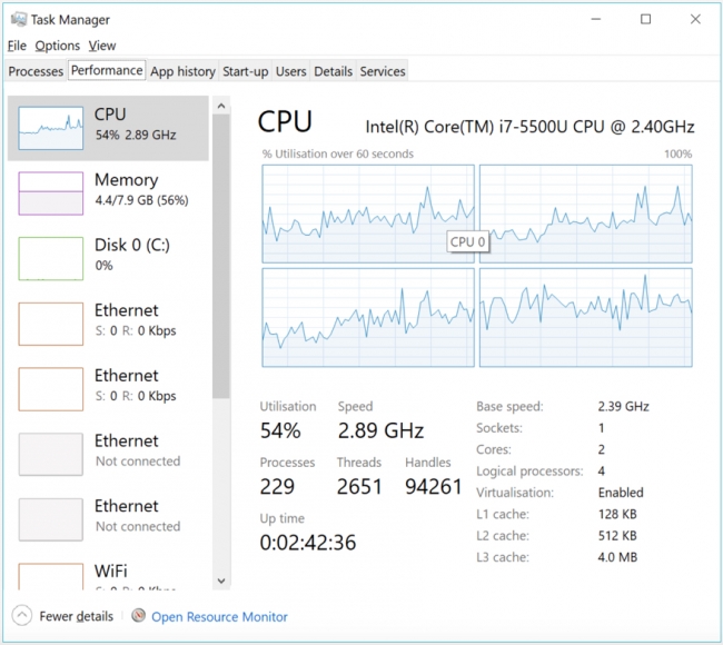
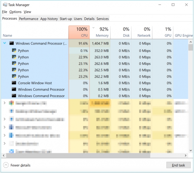
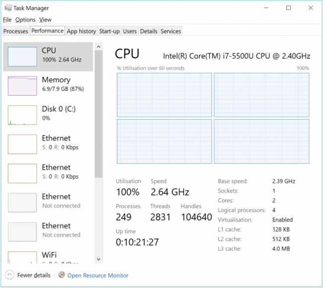
On this four processor PC, this code runs in about 1 second and returns an answer of between 15 and 16. That is about three times slower than my sequential version which ran in 1/3 of a second. If instead I play 1M games instead of 10K games, the parallel version takes 20 seconds on average and my sequential version takes on average 52 seconds. If I run the game 100M times, the parallel version takes around 1,600 seconds (26 minutes) while the sequential version takes 2,646 seconds (44 minutes). The more games I play, the better the performance of the parallel version. Those results aren’t as fast as you might expect with 4 processors in the multiprocessor version but it is still around half the time taken. When we look at profiling our code a bit later in this lesson, we’ll examine why this code isn’t running 4x faster.
When moving the code to a much more powerful PC with 32 processors, there is a much more significant performance improvement. The parallel version plays 100M games in 273 seconds (< 5 minutes) while the sequential version takes 3136 seconds (52 minutes) which is about 11 times slower. Below you can see what the task manager looks like for the 32 core PC in sequential and multiprocessing mode. In sequential mode, only one of the processors is working hard – in the middle of the third row – while the others are either idle or doing the occasional, unrelated background task. It is a different story for the multiprocessor mode where the cores are all running at 100%. The spike you can see from 0 is when the code was started.
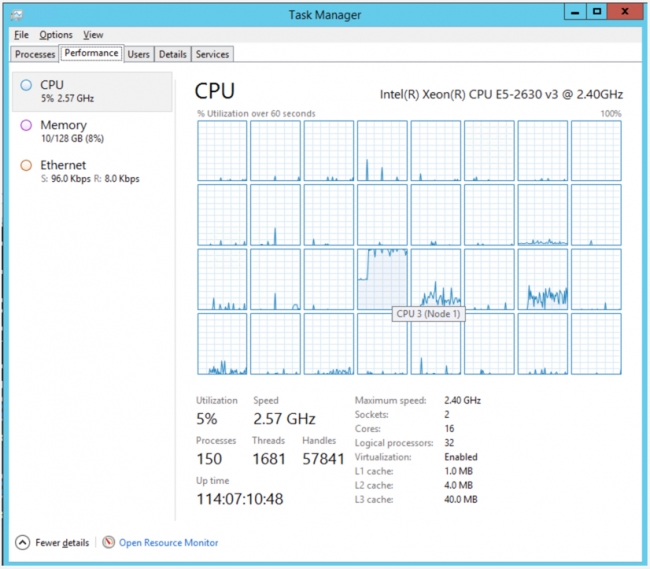
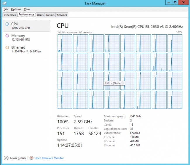
Let's examine some of the reasons for these speed differences. The 4-processor PC’s CPU runs at 3GHz while the 32-processor PC runs at 2.4GHz; the extra cycles that the 4-processor CPU can perform per second make it a little quicker at math. The reason the multiprocessor code runs much faster on the 32-processor PC than the 4-processor PC is straightforward enough –- there are 8 times as many processors (although it isn’t 8 times faster – but it is close at 6.4x (32 min / 5 min)). So while each individual processor is a little slower on the larger PC, because there are so many more, it catches up (but not quite to 8x faster due to each processor being a little slower).
Memory quantity isn’t really an issue here as the numbers being calculated are very small but if we were doing bigger operations, the 4-processor PC with just 8GB of RAM would be slower than the 32-processor PC with 128GB. The memory in the 32-processor PC is also faster at 2.13 GHz versus 1.6GHz in the 4-processor PC.
So the takeaway message here is if you have a lot of tasks that are largely the same but independent of each other, you can save a significant amount of time utilizing all of the resources within your PC with the help of multiprocessing. The more powerful the PC, the more time that can potentially be saved. However, the caveat is that as already noted multiprocessing is generally only faster for CPU-bound processes, not I/O-bound ones.
1.6.6 Arcpy multiprocessing examples
Now that we have completed a non-ArcGIS parallel processing exercise, let's look at a couple of examples using ArcGIS functions. There are a number of caveats or gotchas to using multiprocessing with ArcGIS and it is important to cover them up-front because they affect the ways in which we can write our code.
Esri describe a number of best practices for multiprocessing with arcpy. These include:
- Use “in_memory“ workspaces to store temporary results because as noted earlier memory is faster than disk.
- Avoid writing to file geodatabase (FGDB) data types and GRID raster data types. These data formats can often cause schema locking or synchronization issues. That is because file geodatabases and GRID raster types do not support concurrent writing – that is, only one process can write to them at a time. You might have seen a version of this problem in arcpy previously if you tried to modify a feature class in Python that was open in ArcGIS. That problem is magnified if you have an FGDB and you’re trying to write many feature classes to it at once. Even if all of the feature classes are independent you can only write them to the FGDB one at a time.
- Use 64-bit. This isn’t an issue if we are writing code in ArcGIS Pro (although Esri does recommend using a version of Pro greater than 1.4) because we are already using 64-bit, but if you were planning on using Desktop as well, then you would need to use ArcGIS Server 10.5 (or greater) or ArcGIS Desktop with Background Geoprocessing (64-bit). The reason for this is that as we previously noted 64-bit processes can access significantly more memory and using 64-bit might help resolve any large data issues that don’t fit within the 32-bit memory limits of 4GB.
So bearing the top two points in mind we should make use of in_memory workspaces wherever possible and we should avoid writing to FGDBs (in our worker functions at least – but we could use them in our master function to merge a number of shapefiles or even individual FGDBs back into a single source).
1.6.6.1 Multiprocessing with raster data
There are two types of operations with rasters that can easily (and productively) be implemented in parallel: operations that are independent components in a workflow, and raster operations which are local, focal or zonal – that is they work on a small portion of a raster such as a pixel or a group of pixels.
Esri’s Clinton Dow and Neeraj Rajasekar presented way back at the 2017 User Conference demonstrating multiprocessing with arcpy and they had a number of useful graphics in their slides which demonstrate these two categories of raster operations which we have reproduced here as they're still appropriate and relevant.
An example of an independent workflow would be if we calculate the slope, aspect and some other operations on a raster and then produce a weighted sum or other statistics. Each of the operations is independently performed on our raster up until the final operation which relies on each of them (see the first image below). Therefore, the independent operations can be parallelized and sent to a worker and the final task (which could also be done by a worker) aggregates or summarises the result. Which is what we can see in the second image as each of the tasks is assigned to a worker (even though two of the workers are using a common dataset) and then Worker 4 completes the task. You can probably imagine a more complex version of this task where it is scaled up to process many elevation and land-use rasters to perform many slope, aspect and reclassification calculations with the results being combined at the end.
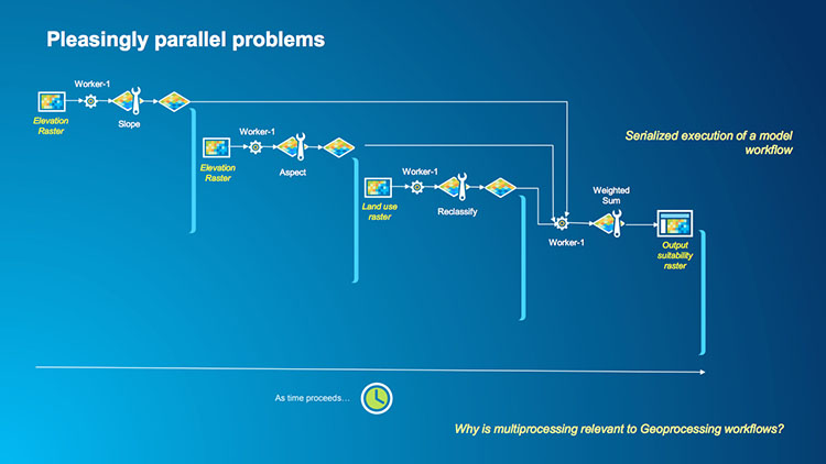
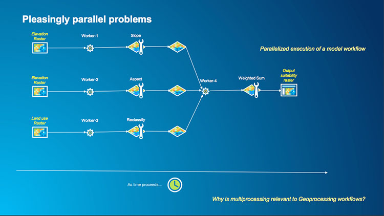
An example of the second type of raster operation is a case where we want to make a mathematical calculation on every pixel in a raster such as squaring or taking the square root. Each pixel in a raster is independent of its neighbors in this operation so we could have multiple workers processing multiple tiles in the raster and the result is written to a new raster. In this example, instead of having a single core serially performing a square root calculation across a raster (the first image below) we can segment our raster into a number of tiles, assign each tile to a worker and then perform the square root operation for each pixel in the tile outputting the result to a single raster which is shown in the second image below.
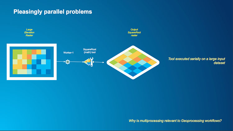

Let‘s return to the raster coding example that we used to build our ArcGIS Pro tool earlier in the lesson. That simple example processed a list of rasters and completed a number of tasks on each raster. Based on what you have read so far I expect that you have realized that this is also a pleasingly parallel problem.
Bearing in mind the caveats about parallel programming from above and the process that we undertook to convert the Cherry-O program, let's begin.
Our first task is to identify the parts of our problem that can work in parallel and the parts which we need to run sequentially.
The best place to start with this can be with the pseudocode of the original task. If we have documented our sequential code well, this could be as simple as copying/pasting each line of documentation into a new file and working through the process. We can start with the text description of the problem and build our sequential pseudocode from there and then create the multiprocessing pseudocode. It is very important to correctly and carefully design our multiprocessing solutions to ensure that they are as efficient as possible and that the worker functions have the bare minimum of data that they need to complete the tasks, use in_memory workspaces, and write as little data back to disk as possible.
Our original task was :
Get a list of raster tiles
For every tile in the list:
     Fill the DEM
     Create a slope raster
     Calculate a flow direction raster
     Calculate a flow accumulation raster
     Convert those stream rasters to polygon or polyline feature classes.
You will notice that I’ve formatted the pseudocode just like Python code with indentations showing which instructions are within the loop.
As this is a simple example we can place all of the functionality within the loop into our worker function as it will be called for every raster. The list of rasters will need to be determined sequentially and we’ll then pass that to our multiprocessing function and let the map element of multiprocessing map each raster onto a worker to perform the tasks. We won’t explicitly be using the reduce part of multiprocessing here as the output will be a featureclass but reduce will probably tidy up after us by deleting temporary files that we don’t need.
Our new pseudocode then will look like :
Get a list of raster tiles
For every tile in the list:
    Launch a worker function with the name of a raster

Worker:
     Fill the DEM
     Create a slope raster
     Calculate a flow direction raster
     Calculate a flow accumulation raster
     Convert those stream rasters to polygon or polyline feature classes.
Bear in mind that not all multiprocessing conversions are this simple. We need to remember that user output can be complicated because multiple workers might be attempting to write messages to our screen at once and that can cause those messages to get garbled and confused. A workaround for this problem is to use Python’s logging library which is much better at handling messages than us manually using print statements. We haven't implemented logging in this sample solution for this script but feel free to briefly investigate it to supplement the print and arcpy.AddMessage functions with calls to the logging function. The Python Logging Cookbook has some helpful examples.
As an exercise, attempt to implement the conversion from sequential to multiprocessing. You will probably not get everything right since there are a few details that need to be taken into account such as setting up an individual scratch workspace for each call of the worker function. In addition, to be able to run as a script tool the script needs to be separated into two files with the worker function in its own file. But don't worry about these things, just try to set up the overall structure in the same way as in the Cherry-O multiprocessing version and then place the code from the sequential version of the raster example either in the main function or worker function depending on where you think it needs to go. Then check out the solution linked below.
Click here for one way of implementing the solution
When you run this code, do you notice any performance differences between the sequential and multiprocessor versions?
The sequential version took 96 seconds on the same 4-processor PC we were using in the Cherry-O example, while the multiprocessor version completed in 58 seconds. Again not 4 times faster as we might expect but nearly twice as fast with multiprocessing is a good improvement. For reference, the 32-processor PC from the Cherry-O example processed the sequential code in 110 seconds and the multiprocessing version in 40 seconds. We will look in more detail at the individual lines of code and their performance when we examine code profiling but you might also find it useful to watch the CPU usage tab in Task Manager to see how hard (or not) your PC is working.
1.6.6.2 Multiprocessing with vector data
The best practices of multiprocessing that we introduced earlier are even more important when we are working with vector data than they are with raster data. The geodatabase locking issue is likely to become much more of a factor as typically we use more vector data than raster and often geodatabases are used more with feature classes.
The example we’re going to use here involves clipping a feature layer by polygons in another feature layer. A sample use case of this might be if you need to segment one or several infrastructure layers by state or county (or even a smaller subdivision). If I want to provide each state or county with a version of the roads, sewer, water or electricity layers (for example) this would be a helpful script. To test out the code in this section (and also the first homework assignment), you can again use the data from the USA.gdb geodatabase (Section 1.5) we provided. The application then is to clip the data from the roads, cities, or hydrology data sets to the individual state polygons from the States data set in the geodatabase.
To achieve this task, one could run the Clip tool manually in ArcGIS Pro but if there are a lot of polygons in the clip data set, it will be more effective to write a script that performs the task. As each state/county is unrelated to the others, this is an example of an operation that can be run in parallel.
The code example below has been adapted from a code example written by Duncan Hornby at the University of Southampton in the United Kingdom that has been used to demonstrate multiprocessing and also how to create a script tool that supports multiprocessing. We will take advantage of Mr. Hornby’s efforts and make use of his code (with attribution of course) but we have also reorganized and simplified it quite a bit and added some enhancements.
Let us examine the code’s logic and then we’ll dig into the syntax.
The code has two Python files. This is important because when we want to be able to run it as a script tool in ArcGIS, it is required that the worker function for running the individual tasks be defined in its own module file, not in the main script file for the script tool with the multiprocessing code that calls the worker function. The first file called scripttool.py imports arcpy, multiprocessing, and the worker code contained in the second python file called multicode.py and it contains the definition of the main function mp_handler() responsible for managing the multiprocessing operations similar to the Cherry-O multiprocessing version. It uses two script tool parameters, the file containing the polygons to use for clipping (variable clipper) and the file to be clipped (variable tobeclipped). Furthermore, the file includes a definition of an auxiliary function get_install_path() which is needed to determine the location of the Python interpreter for running the subprocesses in when running the code as a script tool in ArcGIS. The content of this function you don't have to worry about. The main function mp_handler() calls the worker(...) function located in the multicode file, passing it the files to be used and other information needed to perform the clipping operation. This will be further explained below . The code for the first file including the main function is shown below.
import os, sys
import arcpy
import multiprocessing
from multicode import worker

# Input parameters
clipper = r"C:\489\USA.gdb\States"
#clipper = arcpy.GetParameterAsText(0)
tobeclipped = r"C:\489\USA.gdb\Roads"
#tobeclipped = arcpy.GetParameterAsText(1)

def get_install_path():
    ''' Return 64bit python install path from registry (if installed and registered),
        otherwise fall back to current 32bit process install path.
    '''
    if sys.maxsize > 2**32: return sys.exec_prefix #We're running in a 64bit process

    #We're 32 bit so see if there's a 64bit install
    path = r'SOFTWARE\Python\PythonCore\2.7'

    from _winreg import OpenKey, QueryValue
    from _winreg import HKEY_LOCAL_MACHINE, KEY_READ, KEY_WOW64_64KEY

    try:
        with OpenKey(HKEY_LOCAL_MACHINE, path, 0, KEY_READ | KEY_WOW64_64KEY) as key:
            return QueryValue(key, "InstallPath").strip(os.sep) #We have a 64bit install, so return that.
    except: return sys.exec_prefix #No 64bit, so return 32bit path

def mp_handler():

    try:
        # Create a list of object IDs for clipper polygons

        arcpy.AddMessage("Creating Polygon OID list...")
        print("Creating Polygon OID list...")
        clipperDescObj = arcpy.Describe(clipper)
        field = clipperDescObj.OIDFieldName

        idList = []
        with arcpy.da.SearchCursor(clipper, [field]) as cursor:
            for row in cursor:
                id = row[0]
                idList.append(id)

        arcpy.AddMessage("There are " + str(len(idList)) + " object IDs (polygons) to process.")
        print("There are " + str(len(idList)) + " object IDs (polygons) to process.")

        # Create a task list with parameter tuples for each call of the worker function. Tuples consist of the clippper, tobeclipped, field, and oid values.

        jobs = []

        for id in idList:
            jobs.append((clipper,tobeclipped,field,id)) # adds tuples of the parameters that need to be given to the worker function to the jobs list

        arcpy.AddMessage("Job list has " + str(len(jobs)) + " elements.")
        print("Job list has " + str(len(jobs)) + " elements.")

        # Create and run multiprocessing pool.

        multiprocessing.set_executable(os.path.join(get_install_path(), 'pythonw.exe')) # make sure Python environment is used for running processes, even when this is run as a script tool

        arcpy.AddMessage("Sending to pool")
        print("Sending to pool")

        cpuNum = multiprocessing.cpu_count()  # determine number of cores to use
        print("there are: " + str(cpuNum) + " cpu cores on this machine")

        with multiprocessing.Pool(processes=cpuNum) as pool: # Create the pool object
            res = pool.starmap(worker, jobs)  # run jobs in job list; res is a list with return values of the worker function

        # If an error has occurred report it

        failed = res.count(False) # count how many times False appears in the list with the return values
        if failed > 0:
            arcpy.AddError("{} workers failed!".format(failed))
            print("{} workers failed!".format(failed))

        arcpy.AddMessage("Finished multiprocessing!")
        print("Finished multiprocessing!")

    except arcpy.ExecuteError:
        # Geoprocessor threw an error
        arcpy.AddError(arcpy.GetMessages(2))
        print("Execute Error:", arcpy.ExecuteError)
    except Exception as e:
        # Capture all other errors
        arcpy.AddError(str(e))
        print("Exception:", e)

if __name__ == '__main__':
    mp_handler()
Let's now have a close look at the logic of the two main functions which will do the work. The first one is the mp_handler() function shown in the code section above. It takes the input variables and has the job of processing the polygons in the clipping file to get a list of their unique IDs, building a job list of parameter tuples that will be given to the individual calls of the worker function, setting up the multiprocessing pool and running it, and taking care of error handling.
The second function is the worker function called by the pool (named worker in this example) located in the multicode.py file (code shown below). This function takes the name of the clipping feature layer, the name of the layer to be clipped, the name of the field that contains the unique IDs of the polygons in the clipping feature layer, and the feature ID identifying the particular polygon to use for the clipping as parameters. This function will be called from the pool constructed in mp_handler().
The worker function will then make a selection from the clipping layer. This has to happen in the worker function because all parameters given to that function in a multiprocessing scenario need to be of a simple type that can be "pickled." Pickling data means converting it to a byte-stream which in the simplest terms means that the data is converted to a sequence of simple Python types (string, number etc.). As feature classes are much more complicated than that containing spatial and non-spatial data, they cannot be readily converted to a simple type. That means feature classes cannot be "pickled" and any selections that might have been made in the calling function are not shared with the worker functions. Therefore, we need to think about creative ways of getting our data shared with our sub-processes. In this case, that means we’re not going to do the selection in the master module and pass the polygon to the worker module. Instead, we’re going to create a list of feature IDs that we want to process and we’ll pass an ID from that list as a parameter with each call of the worker function that can then do the selection with that ID on its own before performing the clipping operation. For this, the worker function selects the polygon matching the OID field parameter when creating a layer with MakeFeatureLayer_management() and uses this selection to clip the feature layer to be clipped. The results are saved in a shapefile including the OID in the file's name to ensure that the names are unique.
import os, sys
import arcpy

def worker(clipper, tobeclipped, field, oid):
    """
       This is the function that gets called and does the work of clipping the input feature class to one of the polygons from the clipper feature class.
       Note that this function does not try to write to arcpy.AddMessage() as nothing is ever displayed.  If the clip succeeds then it returns TRUE else FALSE.
    """
    try:
        # Create a layer with only the polygon with ID oid. Each clipper layer needs a unique name, so we include oid in the layer name.
        query = '"' + field +'" = ' + str(oid)
        arcpy.MakeFeatureLayer_management(clipper, "clipper_" + str(oid), query)

        # Do the clip. We include the oid in the name of the output feature class.
        outFC = r"c:\489\output\clip_" + str(oid) + ".shp"
        arcpy.Clip_analysis(tobeclipped, "clipper_" + str(oid), outFC)

        print("finished clipping:", str(oid))
        return True # everything went well so we return True
    except:
        # Some error occurred so return False
        print("error condition")
        return False
Having covered the logic of the code, let's review the specific syntax used to make it all work. While you’re reading this, try visualizing how this code might run sequentially first – that is one polygon being used to clip the to-be-clipped feature class, then another polygon being used to clip the to-be-clipped feature class and so on (maybe through 4 or 5 iterations). Then once you have an understanding of how the code is running sequentially try to visualize how it might run in parallel with the worker function being called 4 times simultaneously and each worker performing its task independently of the other workers.
We’ll start with exploring the syntax within the mp_handler(...) function.
The mp_handler(...) function begins by determining the name of the field that contains the unique IDs of the clipper feature class using the arcpy.Describe(...) function (line 36 and 37). The code then uses a Search Cursor to get a list of all of the object (feature) IDs from within the clipper polygon feature class (line 39 to 43). This gives us a list of IDs that we can pass to our worker function along with the other parameters. As a check, the length of that list is printed out (lines 45 and 46).
Next, we create the job list with one entry for each call of the worker() function we want to make (lines 50 to 53). Each element in this list is a tuple of the parameters that should be given to that particular call of worker(). This list will be required when we set up the pool by calling pool.starmap(...). To construct the list, we simply loop through the ID list and append a parameter tuple to the list in variable jobs. The first three parameters will always be the same for all tuples in the job list; only the polygon ID will be different. In the homework assignment for this lesson, you will adapt this code to work with multiple input files to be clipped. As a result, the parameter tuples will vary in both the values for the oid parameter and for the tobeclipped parameter.
To prepare the multiprocessing pool, we first specify what executable should be used each time a worker is spawned (line 60). Without this line, a new instance of ArcGIS Pro would be launched by each worker, which is clearly less than ideal. Instead, this line calls the get_install_path() function defined in lines 12-27 to determine the path to the pythonw.exe executable.
The code then sets up the size of the pool using the maximum number of processors in lines 65-68 (as we have done in previous examples) and then, using the starmap() method of Pool, calls the worker function worker(...) once for each parameter tuple in the jobs list (line 69).
Any outputs from the worker function will be stored in variable res. These are the boolean values returned by the worker() function, True to indicate that everything went ok and False to indicate that the operation failed. If there is at least one False value in the list, an error message is produced stating the exact number of worker processes that failed (lines 73 to 76).
Let's now look at the code in our worker function worker(...). As we noted in the logic section above, it receives four parameters: the full paths of the clipping and to-be-clipped feature classes, the name of the field that contains the unique IDs in the clipper feature class, and the OID of the polygon it is to use for the clipping.
Notice that the MakeFeatureLayer_management(...) function in line 12 is used to create an in_memory layer which is a copy of the original clipper layer. This use of the in_memory layer is important in three ways: The first is performance – in_memory layers are faster; second, the use of an in_memory layer can help prevent any chance of file locking (although not if we were writing back to the file); third, selection only works on layers so even if we wanted to, we couldn’t get away without creating this layer.
The call of MakeFeatureLayer_management(...) also includes an SQL query string defined one line earlier in line 11 to create the layer with just the polygon that matches the oid that was passed as a parameter. The name of the layer we are producing here should be unique; this is why we’re adding str(oid) to the name in the first parameter.
Now with our selection held in our in_memory, uniquely named feature layer, we perform the clip against our to-be-clipped layer (line 16) and store the result in outFC which we define in line 15 to be a hardcoded folder with a unique name starting with "clip_" followed by the oid. To run the code, you will most likely have to adapt the path used in variable outFC.
The process then returns from the worker function and will be supplied with another oid. This will repeat until a call has been made for each polygon in the clipping feature class.
We are going to use this code as the basis for our Lesson 1 homework project. Have a look at the Assignment Page for full details.
You can test this code out by running it in a number of ways. If you run it from ArcGIS Pro as a script tool, you will have to swap the hashmarks for the clipper and tobeclipped input variables so that GetParameterAsText() is called instead of using hardcoded paths and file names. Be sure to set your parameter type for both parameters to Feature Class. If you make changes to the code and have problems with the changes to the code not being reflected in Pro, delete your Script tool from the Toolbox, restart Pro and re-add the script tool.
You can run your code from spyder but only if you hardcode your parameters or supply them from spyder (Run>Run configuration per file, tick the Command line options checkbox and then enter your filenames separated by a space in the text box alongside. Also make sure you're running the scripttool.py in spyder (not the multicode.py). You can also run your code from the Command Prompt which is the fastest way with the smallest resource overhead.
The final thing to remember about this code is that it has a hardcoded output path defined in variable outFC in the worker() function - which you will want to change, create and/or parameterize etc. so that you have some output to investigate. If you do none of these things then no output will be created.
When the code runs it will create a shapefile for every unique object identifier in the "clipper" shapefile (there are 51 in the States data set from the sample data) named using the OID (that is clip_1.shp - clip_59.shp).
1.7 Debugging and profiling
Debugging and profiling are important skills for any serious programmer – debugging helps you step through your code and helps you analyze the contents of variables (watches) and set breakpoints to check code progress. Profiling runs code to provide an in-depth breakdown of the execution times of individual lines of code or blocks of code to identify performance bottlenecks in the code (e.g. slow I/O, inefficient loops etc.)
In this section, we will first examine debugging techniques and processes before investigating code profiling (which is required for the Lesson 1 Homework Assignment).
1.7.1 Debugging
As you may remember from GEOG 485, the simplest method of debugging is to embed print statements in your code to either determine how far your code is running through a loop or to print out the contents of a variable.
A more complicated and detailed method involves using the tools or features of your IDE to create watches for checking the contents of variables and breakpoints for stepping through your code. While we will introduce a range of IDEs at the end of the lesson and you will be investigating IDEs further and examining how their debugging tools work, we will provide a generic overview of the techniques here of setting watches, breakpoints and stepping through code. Don’t focus on the specifics of the interface as we do this. Instead, it is more important to understand the purpose of each of the different methods of debugging. While we could examine debugging using IDLE (or PythonWin as we did in GEOG 485) we’ve chosen to use a more representative IDE – Spyder as it more accurately demonstrates the features available in the majority of IDEs and you should also already have it installed from earlier.
We will start off by looking at Spyder’s debugging functions, which are similar to those of PythonWin from GEOG 485 and all other IDEs. You might remember back in GEOG 485 when we looked at debugging we examined setting up breakpoints, watches, and stepping through code. We’re going to revisit those concepts here briefly using Spyder; the same functionality will be available in all of the IDEs you’ll be investigating later but you might have to dig a little in the menus for it. There's more details in the Spyder help here.
For our debugging and profiling with Spyder, we’re going to use our raster multiprocessing example (the one that involved delineating streams from lidar data) from earlier. After starting Spyder and opening that file, click on the Debug menu and you will see a number of options.
Set the cursor to the line of code which filters our list of rasters :
new_rasters = filter_list(rasters,wildCardList)
and set a breakpoint by choosing Set/Clear breakpoint from the Debug menu or pressing F12 or double-clicking alongside the line number of the code where you want a breakpoint (removing breakpoints uses the same methods as adding them).
Now run your code using the Debug item from the Debug menu, by pressing CTRL+F5, or using the  button. Your code will now start running and then pause prior to running the line of code at your breakpoint.
One of the nice touches to Spyder is that it has a variable explorer pane, accessible from the View > Panes menu. This will show you a list of your variables, their type, size, and contents once they’re declared, and you can watch them change.
If you bring this pane up you will see two variables already in it, start_time and rasters, our list which has a size of 43 – that is 43 elements - so the code found 43 rasters in my case.
We can step to the next line of code using either Debug>Step, CTRL+F10, or the Step button  . Notice that when you do this, an extra variable will appear in your list (new_rasters) and your next executable line of code will be highlighted in a pale grey band.
We can step through our code line by line to monitor its state as well as the contents of our variables to ensure that our code is doing what we expect it to. While we are doing this, we are looking for unexpected results in variables, loops that are not running correctly (either doing too many or too few iterations or not at all) and if/elif/else statements which are not being correctly evaluated.
While we can step through lines individually, there are also two more useful options in most IDEs which are "run current function until it returns" and "run to the next breakpoint." Spyder has these implemented using the buttons  and
and  , respectively, and I suggest that you experiment with both to see how your functions are executed – particularly with the multiprocessing code. If you want to run between multiple breakpoints, you will need to add some more breakpoints to your code, otherwise, the code will run to the end.
Lastly, if you don’t want to step through all of the lines of code in a function, you can use the Step Return button , which will return you to the calling function.
1.7.2 Profiling
We have experimented with some very simple code profiling by introducing the time() function into our code in previous examples using it to record the start and end times of our code and check the overall performance.
While that gives us a high level view of the performance of our code, we do not know where specific bottlenecks might exist within that code. For example what is the slowest part of our algorithm, is it the file reading or writing or the calculations in between? When we know where these bottlenecks are we can investigate ways of removing them or at least using faster techniques to speed up our code.
In this section, we will focus on basic profiling that looks at how long each function call takes – not each individual line of code. This basic type of code profiling is built into Spyder (and most IDEs). However, we also provide some complementary materials that explain how to visualize profiling results and on how to profile each line of code individually but these parts will be entirely optional because they are quite a bit more complex and require the installation of additional software and packages. It is possible that you will run into some technical/installation issues, so our recommendation is that you only come back and try to run the described steps in these optional subsections yourself if you are done with lesson and homework assignment and still have time left.
1.7.2.1 Basic code profiling
We will again use the Spyder IDE and our basic raster code from earlier in the lesson. Spyder has a Profile pane as well which is accessible from the View -> Panes menu. You may need to manually load your code into Profiler using the folder icon. The spyder help for the Profiler is here if you'd like to read it (Profiler — Spyder 5 documentation (spyder-ide.org)) but we explain the important parts below.
Once you load your code, Profiler automatically starts profiling it and displays the message “ Profiling, please wait...“ at the top of the Profiler window. You will need to be a little patient as Spyder runs through all of your code to perform the timing (or alternatively in these raster examples reduce the sample size). You probably remember that we recommended to run multiprocessing code from the command line rather than inside Spyder. However, using the built-in profiler for loading and running multiprocessing code works as long as the worker function is defined in its own module as we did for the vector clipping example to be able to use it as a script tool. If this is not the case, you will receive an error that certain elements in the code cannot be “pickled“ which you might remember from our multiprocessing discussion means those objects cannot be converted to a basic type. We didn't split the multiprocessing version of the raster example into two separate modules, so here we will only look at the non-multiprocessing version and profile that. We won't have this issue when we using other profilers in the following optional sections and in the homework assignment you will work with the vector clipping multiprocessing example which has been set up in a way that allows for profiling with the Spyder profiler.
Once the Profiler has completed you will see a set of results like the ones below.
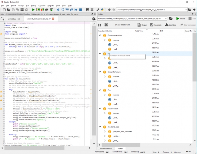
Looking over those results you will see a list of functions together with the times each has taken. The important column to examine is the Local Time column which shows you how long each function has taken to execute in us (microseconds), ms (milliseconds), seconds, minutes etc. The Total Time column is showing you the cumulative time for each of those processes that was run (e.g. if your code was running in a function). You can order any of the columns but if you arrange the Total Time column in ascending order this will give you a logical starting point as the times will be arranged from the shortest to longest running. There is no way to order the results to see the order in which your code ran. So you will see (depending on your code arrangement) overwriteOutput followed by the time function, then filterList, etc.
The next column to look at is the Calls column which has the count of how many times each of those functions was launched. So a high value in Local Time might be indicative of either a large number of calls to a very fast function or a small number of calls to a very slow function.
In my timings, there aren’t any obvious places to look for performance improvements although the code could be fractionally faster (but less of a good team player) if I didn’t check the extension back in and my .replace() method and print add a small amount of time to the execution.
What we are doing with this type of profiling is examining the sum of the functions and methods which were called during the code execution and how long they took, in total, for the number of times that they were called. It is possible to identify inefficiencies with this sort of profiling, particularly in combination with debugging. Am I calling a slow function too often? Can I find a faster function to do the same job (for example some mathematical functions are significantly faster than others and achieve the same result and often there exist approximations that give almost the exact result but are much faster to compute)?
It is worth pointing out here that the results from Spyder’s Profiler are actually the output from the cProfile package of the Python standard library which is essentially wrapped around our script to calculate the statistics we are seeing above. You could import this package into your own code and use it there directly but we will focus on using its functionality from the IDE which is usually more convenient and the results are presented in a more readily understood format.
You might be thinking that these results aren’t really that readily understood and it would be easier if there were a graphical visualization of the timings. Luckily there is and if you want to learn more about it, the following optional sections on code profiling with visualiuation are a good starting point. In addition, we continue another optional section that explains how you can do more detailed profiling looking at each individual line rather than complete functions. However, we recommend that you skip or only skim through these optional sections on your first pass through the lesson materials and come back when you have the time.
1.7.2.2 Optional complementary materials: Code profiling with visualizations
As we said at the beginning of this section, this section is provided for interest only. Please feel free to skip over it and you can loop back to it at the end of the lesson if you have free time or after the end of the class. Be warned: installing the required extensions and using them is a little complicated - but this is an advanced class, so don't let this deter you.
We are going to need to download some software called QCacheGrind which reads a tree type file (like a family tree). Unfortunately, QcacheGrind doesn’t natively support the profile files we are going to be creating so we will also need a converter (pyprof2calltree), written in Python. Our workflow is going to be :
- Download & install QCacheGrind (we only need to do this once)
- Use pip (a Python package manager) to install our converter (we only need to do this once, too)
- Run our function and line profiling and save the output to files
- Convert those output profile files using our converter
- Open the converted files in QCacheGrind
- ...
- Conquer Python (okay maybe not, but at least have a better understanding of our code’s performance)
Installing QCacheGrind
Download QCacheGrind and unzip it to a folder. QcacheGrind can be run by double-clicking on the qcachegrind executable in the folder you’ve just unzipped it to. Don’t do that just yet though, we’ll come back to it once we’ve done the other steps in our workflow and when we have some profile files to visualize.
Installing the Converter - pyprof2calltree
Now we’re going to install our converter using the Python Preferred Installer Program, pip. If you would like to learn more about pip, the Python 3 Help (Key Terms) has a full explanation. You will also learn more about Python packet managers in the next lesson. Pip is included by default with the Python installation you have but we have to access it from the Python Command Prompt.
As we mentioned in Section 1.6.5.2, there should be a shortcut within the ArcGIS program group on the start menu called "Python Command Prompt" on your PC that opens a command window running within the conda environment indicating that this is Python 3 (py3). You actually may have several shortcuts with rather similar sounding names, e.g. if you have both ArcGIS Pro and ArcGIS Desktop installed, and it is important that you pick the right one from ArcGIS Pro using Python 3.
In the event that there isn’t a shortcut, you can start Python from a standard Windows command prompt by typing :
"%PROGRAMFILES%\ArcGIS\Pro\bin\Python\Scripts\propy"
The instructions above mirror Esri's help for running Python.
Open your Python command prompt and you should be in the folder C:\Users\<username>\AppData\Local\ESRI\conda\envs\arcgispro-py3-clone\ or C:\Program Files\ArcGIS\Pro\bin\Python\envs\arcgispro-py3\ depending on your version of ArcGIS Pro. This is the default folder when the command prompt opens (which you can see at the prompt). Then type (and hit Enter) :
Scripts\pip install pyprof2calltree
Pip will then download from a repository of hosted Python packages the converter that we need and then install it. You should see a message saying “Successfully installed pyprof2calltree-1.4.3“ although your version number may be higher and that’s ok. If you receive an error message about permissions during the pyprof2calltree installation, close out of Python command prompt and reopen the program with administrative privileges (usually right-clicking on the program and selecting "Run as administrator," in Windows 10, you might need to "Open File Location" and then right-click to "Run as administrator").
After running commands in Python command prompt, you will probably also see an information message stating:
“You are using pip version 9.0.3, however version 10.0.1 is available. You should consider upgrading via the `python –m pip install –upgrade pip‘ command.“
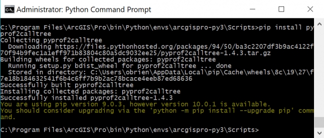
You can ignore this message, we’re going to leave pip at its current version as that is what came with the ArcGIS Pro Python distribution and we know that it works.
1.7.2.3 Optional complementary materials: Code profiling with visualizations (continued)
This section is provided for interest only. Please feel free to skip over it and you can loop back to it at the end of the lesson if you have free time or after the end of the class.
Creating profile files
Now that we have the QCacheGrind viewer and converter installed we can create some profile files and we'll do that using IPython (available on another tab in Spyder). Think of IPython a little like the interactive Python window in ArcGIS with a few more bells and whistles. We’ll use IPython very shortly for line-by-line profiling, so as a bridge to that task, let's use it to perform some more simple profiling.
Open the IPython pane in Spyder and then you will probably need to change to the folder where your code is located. This should be as easy as looking at the top of the Spyder window, selecting and copying the folder name where your code is, then clicking in the IPython window and typing cd and pasting in the folder name and hitting enter (as seen below).
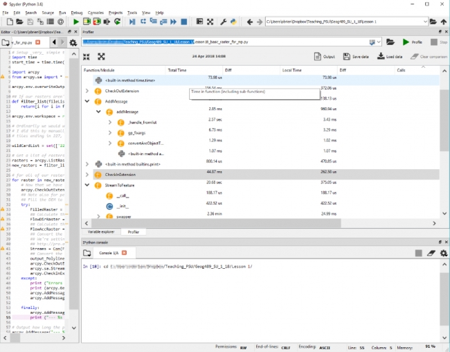
This might look like:
cd c:\Users\YourName\Documents\GEOG489\Lesson1\
We could (but won't) run our code from IPython by typing:
run Lesson1B_basic_raster_for_mp.py
and hitting enter and our code will run and display its output in the IPython window.
That is somewhat useful, but more useful is the ability to use additional packages within IPython for more detailed profiling. Let’s create a function-level profile file using IPython for that raster code and then we’ll run it through the converter and then visualize it in QCacheGrind.
To create that function-level profile we’ll use the built-in profiler prun.
We’ll access it using is a magic word instruction to Spyder which is shorthand for loading an external package; that package is called line_profiler which we just installed. Think of it in the same way as import for Python code – we’re now going to be able to access functionality embedded within that package.
Our magic words have % in front of them. Let's use it to see what the parameters are for using prun with (the ? on the end tells prun to show us its built-in help):
%prun?
If you scroll back up through the IPython console, you will be able to see all of the options for prun. You can compare our command below to that list to break down the various options and experiment with others if you wish. Notice the very last line of the help which states:
If you want to run complete programs under the profiler's control, use "%run -p [prof_opts] filename.py [args to program]" where prof_opts contains profiler specific options as described here.
That is what we’re going to do – use run with the prun options.
cd "C:\Users\YourName"

%run -p -T profile_run.txt -D profile_run.prof
Lesson1B_basic_raster_for_mp
There are a couple of important things to note in these commands. The first is the double quotes around the full path name in the cd command – these are important: just in case there is a space in your path, the double quotes encapsulate it so your folder is found correctly. The other thing is the casing of the various parameters (remember Python is case-sensitive and so are a lot of the built-in tools).
It could take a little while to complete our profiling as our code will run through from start to end. We can check that our code is running by opening the Windows Task Manager and watching the CPU usage which is probably at 100% on one of our cores.
While our code is running we’ll see the normal output with the timing print functions we had implemented earlier. When the run command completes we’ll see a few lines of output that look like :
%run -p -T profile_run.txt -D profile_run.prof
Lesson1B_basic_raster_for_mp

*** Profile stats marshalled to file 'profile_run.prof'.

*** Profile printout saved to text file 'profile_run.txt'.
         3 function calls in 0.000 seconds

   Ordered by: internal time

   ncalls  tottime  percall  cumtime  percall
filename:lineno(function)

        1    0.000    0.000    0.000    0.000 {built-in method
builtins.exec}
        1    0.000    0.000    0.000    0.000
...
        1    0.000    0.000    0.000    0.000
SSL.py:677(Session)
        1    0.000    0.000    0.000    0.000
cookiejar.py:1753(LoadError)
        1    0.000    0.000    0.000    0.000
socks.py:127(ProxyConnectionError)
        1    0.000    0.000    0.000    0.000
_conditional.py:177(cryptography_has_mem_functions)
        1    0.000    0.000    0.000    0.000
_conditional.py:196(cryptography_has_x509_store_ctx_get_issuer)
        1    0.000    0.000    0.000    0.000
_conditional.py:210(cryptography_has_evp_pkey_get_set_tls_enco
dedpoint)
These summary outputs will also be written to a text file that we can open in a text editor (or in Spyder) and our profile file which we will convert and open in QCacheGrind. Writing that output to a text file is useful because there is too much of it to fit within IPython’s window buffer, and you won’t be able to get back to the output right at the start of the execution. If you open the profile_run.txt file in Spyder you’ll see the full output.
Convert output profile files with pyprof2calltree
We’ll run the converter using some familiar Python commands and the convert function within the IPython window:
from pyprof2calltree import convert, visualize
convert('profile_run.prof','callgrind.profile_run')
Open the converted files in QCacheGrind and inspect graphs
The converted output file can now be opened in QCacheGrind. Open QCacheGrind from the folder you installed it into earlier by double-clicking its icon. Click the folder icon in the top left of QCacheGrind or choose File ->Open from the menu and open the callgrind.profile_run file we just created, which should be in the same folder as your source code.
What we have now is a complicated and detailed interface and visualization of every function that our code called but in a more graphically friendly format than the original text file. We can sort by time, number of times a function was called, the function name and the location of that code (our own, within the arcpy library or another library) in the left-hand pane of the interface.
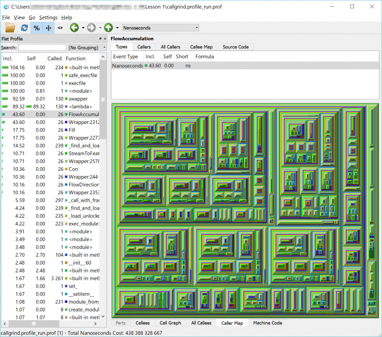
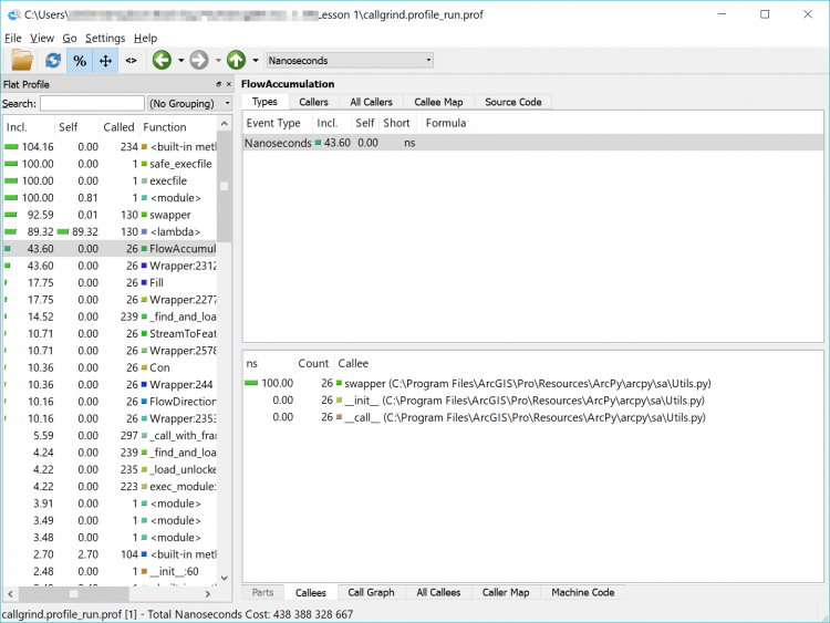
In the list, you will see a lot of built-in functions (things that Python does behind the scenes or that arcpy has it do – calculations, string functions etc.) but you will also see the names of some of the arcpy functions that we used such as FlowAccumulation(...) or StreamToFeature(...). If you double-click on one of them and click on the Call Graph tab in the lower pane you will see a graphical representation of where the tasks were called from. If you double-click on the function’s box above it in the Call Graph pane
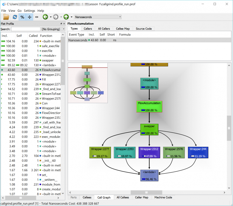
In the example below, we can see that FlowAccumulation(...) is the slowest of our tasks taking about 43% of the execution time. If we can find a way to speed up (or eliminate this process), we’ll make our code more efficient. If we can’t – that’s ok too – we’ll just have to accept that our code takes a certain amount of time to run.
Spend a little time clicking around in the interface and exploring your code – don’t worry too much about going down the rabbit hole of optimizing your code – just explore. Check out functions whose name you recognize such as those raster ones, or ListRasters(). Experiment with examining the content of the different tabs and seeing which modules call which functions (Callers, All Callers and Callee Map). Click down deep into one of the modules and watch the Callee Map change to show each small task being undertaken. If you get too far down the rabbit hole you can use the up arrow near the menu bar to find your way back to the top level modules.
If you’re interested, feel free to run through the process again with your multiprocessing code and see the differences. As a quick reminder, the IPython commands are (although your filenames might be different and be sure to double-check that you're in the correct folder if you get file not found errors):
%run -p -T profile_run_mp.txt -D profile_run_mp.prof Lesson1B_basic_raster_using_mp

from pyprof2calltree import convert, visualize
convert('profile_run_mp.prof','callgrind.profile_run_mp')
If you load that newly created file into QCacheGrind, you’ll note it looks a little different – like an Escher drawing or a geometric pattern. That is the representation of the multiprocessing functions being run. Feel free to explore among here as well – and you will notice that the functions we previously saw are harder to find – or invisible.
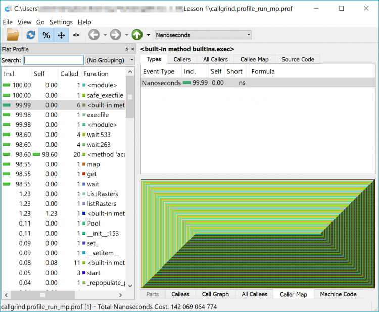
I haven't forgotten about my promise from earlier in the lesson to review the reasons why the Cherry-O code is only about 2-3x faster in multiprocessing mode than the 4x that we would have hoped.
Feel free to run both versions of your Cherry-O code against the profiler and you'll notice that most of the time is taken up by some code described as {method 'acquire' of '_thread.lock' objects} which is called a small number of times. This doesn't give us a lot of information but does hint that perhaps the slower performance is related to something to do with handling multiprocessing objects.
Remember back to our brief discussion about pickling objects which was required for multiprocessing?
It's the culprit, and the following optional section on line profiling will take a closer look at this issue. However, as we said before, line profiling adds quite a bit of complexity, so feel free to skip this section entirely or get back to it after you have worked through the rest of the lesson.
1.7.2.4 Optional complementary materials: Line profiling
As we said at the beginning of this section, this section is provided for interest only. Please feel free to skip over it and you can loop back to it at the end of the lesson if you have free time or after the end of the class. Be warned: installing the required extensions and using them is a little complicated - but this is an advanced class, so don't let this deter you.
Before we begin this optional section, you should know that line profiling is slow – it adds a lot of overhead to our code execution and it should only be done on functions that we know are slow and we’re trying to identify the specifics of why they are slow. Due to that overhead, we cannot rely on the absolute timing reported in line profiling, but we can rely on the relative timings. If a line of code is taking 50% of our execution time and we can reduce that to 40,30 or 20% (or better) of our total execution time then we have been successful.
With that warning about the performance overhead of line profiling, we’re going to install our line profiler (which isn’t the same one that Spyder or ArcGIS Pro would have us install) again using pip (although you are welcome to experiment with those too).
Setting PermissionsBefore we start installing packages we will need to adjust operating system (Windows) permissions on the Python folder of ArcGIS Pro, as we will need the ability to write to some of the folders it contains. This will also help us if we inadvertently attempt to create profile files in the Python folder as the files will be created instead of producing an error that the folder is inaccessible (but we shouldn't create those files there as it will add clutter).
Open up Windows Explorer and navigate to the c:\Program Files\ArcGIS\Pro\bin folder. Select the Python folder and right click on it and select Properties. Select the Security tab, and click the Advanced button. In the new window that opens select Change Permissions, Select the Users group, Uncheck the Include inheritable permissions from this object’s parent box or Disable Inheritance – depending on your version of Windows, and select Add (or Make Explicit) on the dialog that appears.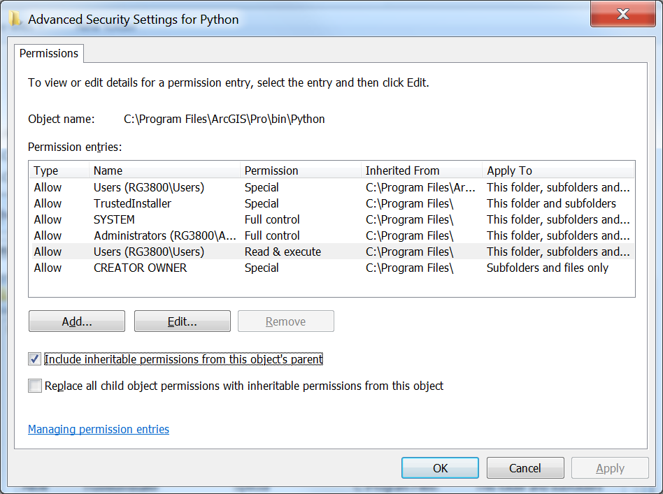
Once again open (if it isn’t already) your Python command prompt and you should be in the folder C:\Program Files\ArcGIS\Pro\bin\Python\envs\arcgispro-py3 or C:\Users\<username>\AppData\Local\ESRI\conda\envs\arcgispro-py3-clone, the default folder of your ArcGIS Pro Python environment, when that command prompt opens (which you can see at the prompt). If in your version of Pro, the command prompt instead shows C:\Users\<username>\AppData\Local\ESRI\conda\envs\arcgispro-py3-clone, then you will have to use this path instead in some of the following commands where the kernprof program is used.
Then type :
scripts\pip install line_profiler
Pip will then download from a repository of hosted Python packages the line_profiler that we need and then install it.
If you receive an error that "Microsoft Visual C++ 14.0 is required," visit https://www.visualstudio.com/downloads/ and download the package for "Visual Studio Community 2017" which will download Visual Studio Installer. Run Visual Studio Installer, and under the "Workloads" tab, you will select two components to install. Under Windows, check the box in the upper right hand corner of "Desktop Development with C++," and, under Web & Cloud, check the box for "Python development." After checking the boxes, click "Install" in the lower right hand corner. After installing those, open the Python command prompt again and enter:
scripts\pip install misaka
If that works, then install the line_profiler with...
scripts\pip install line_profiler
You should see a message saying "Successfully installed line_profiler 2.1.2" although your version number may be higher and that’s okay.
Now that IPython is aware of the line profiler we can run it. There are two modes for running the line profiler, function mode, where we supply a Python file and a function we want to run as well as the parameters for that function given as parameters to the profiler, and module mode, where we supply the module name.
Function-level line profiling is very useful when you want to test just a single function, or if you’re doing multiprocessing as we saw above. Module-level line profiling is a useful first pass to identify those functions that might be slowing things down and it's why we did a similar approach with our higher-level profiling earlier.
Now we can dive into function-level profiling to find the specific lines which might be slowing down our code and then optimize or enhance them and then perform further function-level line profiling (or module-level profiling) again to test our improvements.
We will start with module-level profiling using our single processor Cherry-O code, look at our non-multiprocessing raster example code that did the analysis of the Penn State campus, and finally move on to the multiprocessing Cherry-O code. You may notice a few little deviations in the code that is being used in this section compared to the versions presented in Section 1.5 and 1.6. These deviations are really minimal and have no effect on how the code works and the insights we gain from the profiling.
Our line profiler is in a package called KernProf (named after its author) and it works as a wrapper around the standard cProfile and Line_Profiler tools.
We need to make some changes to our code so that the line profiler knows which functions we wish it to interrogate. The first of those changes is to wrap a function definition around our code (so that we have a function to profile instead of just a single block of code). The second change we need is to use a decorator which is an instruction or meta information for a piece of code that will be ignored by Python. In the case of our profiler, we need to use the decorator @profile to tell KernProf which functions (and we can do many) to examine and it will ignore any without a decorator. Your decorator may give you errors if you're not running your code against the profiler so in that case comment it out.
We’ve made those changes to our original Cherry-O code below so you can see them for yourselves. Check out line 8 for the decorator, line 9 for the function definition (and note how the code is now indented within the function) and line 53 where the function is called. You might also notice that I reduced the number of games back down to 10001 from our very large number earlier. Don’t forget to save your code after you make these changes.
# Simulates 10K game of Hi Ho! Cherry-O
# Setup _very_ simple timing.
import time
start_time = time.time()

import random

@profile
def cherryo():
    spinnerChoices = [-1, -2, -3, -4, 2, 2, 10]
    turns = 0
    totalTurns = 0
    cherriesOnTree = 10
    games = 0

    while games < 10001:
        # Take a turn as long as you have more than 0 cherries
        cherriesOnTree = 10
        turns = 0
        while cherriesOnTree > 0:

            # Spin the spinner
            spinIndex = random.randrange(0, 7)
            spinResult = spinnerChoices[spinIndex]

            # Print the spin result
            #print ("You spun " + str(spinResult) + ".")

            # Add or remove cherries based on the result
            cherriesOnTree += spinResult

            # Make sure the number of cherries is between 0 and 10
            if cherriesOnTree > 10:
                cherriesOnTree = 10
            elif cherriesOnTree < 0:
                cherriesOnTree = 0

            # Print the number of cherries on the tree
            #print ("You have " + str(cherriesOnTree) + " cherries on your tree.")

            turns += 1
        # Print the number of turns it took to win the game
        #print ("It took you " + str(turns) + " turns to win the game.")
        games += 1
        totalTurns += turns

    print ("totalTurns "+str(float(totalTurns)/games))
    #lastline = raw_input(">")

    # Output how long the process took.
    print ("--- %s seconds ---" % (time.time() - start_time))

cherryo()
We could try to run the profiler and the other code from within IPython but that often causes issues such as unfound paths, files, etc., as well as making it difficult to convert our output to a nice readable text file. Instead, we’ll use our Python command prompt and then we’ll run the line profiler using (note: the "-l" is a lowercase L and not the number 1):
python "c:\program files\arcgis\pro\bin\python\envs\arcgispro-py3\lib\site-packages\kernprof.py" -l “c:\users\YourName\CherryO.py”
When the profiling completes (and it will be fast in this simple example), you’ll see our normal code output from our print functions and the summary from the line profiler:
Wrote profile results to CherryO.py.lprof
This tells us the profiler has created an lprof file in our current directory called CherryO.py.lprof (or whatever our input code was called).
The profile files will be saved wherever your Python command prompt path is pointing. Unless you've changed the directory, the Python command prompt will most likely be pointing to C:\Program Files\ArcGIS\Pro\Bin\Python\envs\arcgispro-py3, and the files will be saved in that folder.
The profile files are binary files that will be impossible for us to read without some help from another tool. So to rectify that we’ll run that .lprof file through the line_profiler (which seems a little confusing because you would think we just created that file with the line_profiler and we did, but the line_profiler can also read the files it created) and then pipe (redirect) the output to a text file which we’ll put back in our code directory so we can find it more easily.
To achieve this, we run the following command in our Python command window:
..\python –m line_profiler CherryO.py.lprof > "c:\users\YourName\CherryO.profile.txt"
This command will instruct Python to run the line_profiler (which is some Python code itself) to process the .lprof file we created. The > will redirect the output to a text file at the provided path instead of displaying the output to the screen.
We can then open the resulting output file which should be back in our code folder from within Spyder and read the results. I’ve included my output for reference below and they are also in the CherryO.Profile pdf.
Timer unit: 4.27655e-07 s

Total time: 3.02697 s
File: c:\users\YourName\Lesson 1\CherryO.py
Function: cherryo at line 8

Line #      Hits         Time  Per Hit   % Time  Line Contents
==============================================================
     8                                           @profile
     9                                           def cherryo():
    10         1          5.0      5.0      0.0      spinnerChoices = [-1, -2, -3, -4, 2, 2, 10]
    11         1          2.0      2.0      0.0      turns = 0
    12         1          1.0      1.0      0.0      totalTurns = 0
    13         1          1.0      1.0      0.0      cherriesOnTree = 10
    14         1          1.0      1.0      0.0      games = 0
    15
    16     10002      36775.0      3.7      0.5      while games < 10001:
    17                                                   # Take a turn as long as you have more than 0 cherries
    18     10001      25568.0      2.6      0.4          cherriesOnTree = 10
    19     10001      27091.0      2.7      0.4          turns = 0
    20    168060     464529.0      2.8      6.6          while cherriesOnTree > 0:
    21
    22                                                       # Spin the spinner
    23    158059    4153276.0     26.3     58.7              spinIndex = random.randrange(0, 7)
    24    158059     487698.0      3.1      6.9              spinResult = spinnerChoices[spinIndex]
    25
    26                                                       # Print the spin result
    27                                                       #print "You spun " + str(spinResult) + "."
    28
    29                                                       # Add or remove cherries based on the result
    30    158059     460642.0      2.9      6.5              cherriesOnTree += spinResult
    31
    32                                                       # Make sure the number of cherries is between 0 and 10
    33    158059     458508.0      2.9      6.5              if cherriesOnTree > 10:
    34     42049     112815.0      2.7      1.6                  cherriesOnTree = 10
    35    116010     325651.0      2.8      4.6              elif cherriesOnTree < 0:
    36      5566      14506.0      2.6      0.2                  cherriesOnTree = 0
    37
    38                                                       # Print the number of cherries on the tree
    39                                                       #print "You have " + str(cherriesOnTree) + " cherries on your tree."
    40
    41    158059     445969.0      2.8      6.3              turns += 1
    42                                                   # Print the number of turns it took to win the game
    43                                                   #print "It took you " + str(turns) + " turns to win the game."
    44     10001      29417.0      2.9      0.4          games += 1
    45     10001      31447.0      3.1      0.4          totalTurns += turns
    46
    47         1        443.0    443.0      0.0      print ("totalTurns "+str(float(totalTurns)/games))
    48                                               #lastline = raw_input(">")
    49
    50                                               # Output how long the process took.
    51         1       3723.0   3723.0      0.1      print ("--- %s seconds ---" % (time.time() - start_time))
What we can see here are the individual times to run each line of code: The numbers on the left are the code line numbers, the number of times each line was run (Hits), the time each line took in total (Hits * Time Per Hit), the time per hit, the percentage of time those lines took and, for reference, the line of code alongside.
The first thing that jumps out at me is that the random number selection (line 23) takes the longest time and is called the most – if we can speed this up somehow we can improve our performance.
Let’s move onto the other examples of our code to see some more profiling results.
First we’ll look at the sequential version of our raster processing code before coming back to look at the multiprocessing examples as they’re a little special.
As before with the Cherry-O example we’ll need to wrap our code into a function and use the @profile decorator (and of course call the function). Attempt to make these changes on your own and if you get stuck you can find my code sample here if you want to check your work against mine.
We’ll run the profiler again, produce our output file and then convert it to text and review the results using:
python "c:\program files\arcgis\pro\bin\python\envs\arcgispro-py3\lib\site-packages\kernprof.py" -l "c:\users\YourName\Lesson1B_basic_raster_for_mp.py"
and then
..\python –m line_profiler Lesson1B_basic_raster_for_mp.py.lprof > "c:\users\YourName\Lesson1B_basic_raster_for_mp.py_profile.txt"
If we investigate these outputs (my outputs are here) we can see that the Flow Accumulation calculation is again the slowest, just as we saw when we were doing the module-level calculations. In this case, because we’re predominantly using arcpy functions, we’re not seeing as much granularity or resolution in the results. That is, we don’t know why Flow Accumulation(...) is so slow but I’m sure you can see that in some other circumstances, you could identify multiple arcpy functions which could achieve the same result – and choose the most efficient.
Next, we’ll look at the multiprocessing example of the Cherry-O example to see how we can implement line profiling into our multiprocessing code. As we noted earlier, multiprocessing and profiling are a little special as there is a lot going on behind the scenes and we need to very carefully select what functions and lines we’re profiling as some things cannot be pickled.
Therefore what we need to do is use the line profiler in its API mode. That means instead of using the line profiling outside of our code, we need to embed it in our code and put it in a function between our map and the function we’re calling. This will give us output for each process that we launch. Now if we do this for the Cherry-O example we’re going to get 10,000 files – but thankfully they are small so we’ll work through that as an example.
The point to reiterate before we do that is the Cherry-O code runs in seconds (at most) – once we make these line profiling changes the code will take a few minutes to run.
We’ll start with the easy steps and work our way up to the more complicated ones:
import line_profiler
Now let’s define a function within our code to sit between the map function and the called function (cherryO in my version).
We’ll break down what is happening in this function shortly and that will also help to explain how it fits into our workflow. This new function will be called from our mp_handler() function instead of our original call to cherryO and this new function will then call cherryO.
Our new mp_handler function looks like:
def mp_handler():

    myPool = multiprocessing.Pool(multiprocessing.cpu_count())
    ## The Map function part of the MapReduce is on the right of the = and the Reduce part on the left where we are aggregating the results to a list.
    turns = myPool.map(worker,range(numGames))
    # Uncomment this line to print out the list of total turns (but note this will slow down your code's execution
    #print(turns)
    # Use the statistics library function mean() to calculate the mean of turns
    print(mean(turns))
Note that our call to myPool.map now has worker(...) not cherryO(...) as the function being spawned multiple times. Now let's look at this intermediate function that will contain the line profiler as well as our call to cherryO(...).
def worker(game):
    profiler=line_profiler.LineProfiler(cherryO)
    call = 'cherryO('+str(game)+')'
    turns = profiler.run(call)
    profiler.dump_stats('profile_'+str(game)+'.lprof')
    return(turns)
The first line of our new function is setting up the line profiler and instructing it to track the cherryO(...) function.
As before, we pass the variable game to the worker(...) function and then pass it through to cherryO(...) so it can still perform as before. It’s also important that, when we call cherryO(...), we record the value it returns into a variable turns – so we can return that to the calling function so our calculations work as before. You will notice we’re not just calling cherryO(...) and passing it the variable though – we need to pass the variable a little differently as the profiler can only support certain picklable objects. The most straightforward way to achieve that is to encode our function call into a string (call) and then have the profiler run that call. If we don’t do this the profiler will run but no results will be returned.
Just before we send that value back we use the profiler’s function dump_stats to write out the profile results for the single game to an output file.
Don’t forget to save your code after you make these changes. Now we can run through a slightly different (but still familiar) process to profile and export our results, just with different file names. To run this code we’ll use the Python command prompt:
python c:\users\YourName\CherryO_mp.py
Notice how much longer the code now takes to run – this is another reason to wrap the line profiling in its own function. That means that we don’t need to leave it in production code; we can just change the function calls back and leave the line profiling code in place in case we want to test it again.
It's also possible you'll receive several error messages when the code runs, but the lprof files are still created.
Once our code completes, you will notice we have those 10,000 lprof files (which is overkill as they are probably all largely the same). Examine a few of the files if you like by converting them to text files and viewing them in your favorite text editor or Spyder using the following in the Python command prompt:
python –m line_profiler profile_1.lprof > c:\users\YourName\profile_1.txt
If you examine one of those files, you’ll see results similar to:
Timer unit: 4.27655e-07 s

Total time: 0.00028995 s
File: c:\users\obrien\Dropbox\Teaching_PSU\Geog489_SU_1_18\Lesson 1\CherryO_MP.py
Function: cherryO at line 25

Line #      Hits         Time  Per Hit   % Time  Line Contents
==============================================================
    25                                           def cherryO(game):
    26         1         11.0     11.0      1.6      spinnerChoices = [-1, -2, -3, -4, 2, 2, 10]
    27         1          9.0      9.0      1.3      turns = 0
    28         1          8.0      8.0      1.2      totalTurns = 0
    29         1          8.0      8.0      1.2      cherriesOnTree = 10
    30         1          9.0      9.0      1.3      games = 0
    31
    32                                               # Take a turn as long as you have more than 0 cherries
    33         1          9.0      9.0      1.3      cherriesOnTree = 10
    34         1          9.0      9.0      1.3      turns = 0
    35        16         41.0      2.6      6.0      while cherriesOnTree > 0:
    36
    37                                                   # Spin the spinner
    38        15        402.0     26.8     59.3          spinIndex = random.randrange(0, 7)
    39        15         38.0      2.5      5.6          spinResult = spinnerChoices[spinIndex]
    40
    41                                                   # Print the spin result
    42                                                   #print "You spun " + str(spinResult) + "."
    43
    44                                                   # Add or remove cherries based on the result
    45        15         34.0      2.3      5.0          cherriesOnTree += spinResult
    46
    47                                                   # Make sure the number of cherries is between 0 and 10
    48        15         35.0      2.3      5.2          if cherriesOnTree > 10:
    49         4          8.0      2.0      1.2              cherriesOnTree = 10
    50        11         24.0      2.2      3.5          elif cherriesOnTree < 0:
    51                                                       cherriesOnTree = 0
    52
    53                                                   # Print the number of cherries on the tree
    54                                                   #print "You have " + str(cherriesOnTree) + " cherries on your tree."
    55
    56        15         32.0      2.1      4.7          turns += 1
    57                                               # Print the number of turns it took to win the game
    58         1          1.0      1.0      0.1      return(turns)
Arguably we’re not learning anything that we didn’t know from the sequential version of the code – we can still see the randrange() function is the slowest or most time consuming (by percentage) – however, if we didn’t have the sequential version and wanted to profile our multiprocessing code this would be a very important skill.
The same steps to modify our code above would be implemented if we were performing this line profiling on arcpy (or any other) multiprocessing code. The same type of intermediate function would be required, we would need to pass and return parameters (if necessary) and also reformat the function call so that it was picklable. The output from the line profiler is delivered in a different format to the module-level profiling we were doing before and, therefore, isn’t suitable for loading into QCacheGrind. I'd suggest that isn't as important as we're looking at a much smaller number of lines of code, so the graphical representation isn't as important.
Returning to our ongoing discussion about the less than anticipated performance improvement between our sequential and multiprocessing Cherry-O code, what we can infer by comparing the line profile output of the sequential version of our code and the multiprocessing version is that pretty much all of the steps take the same proportion of time. So if we're doing nearly everything in about the same proportions, but 4 times as many of them (using our 4 processor PC example) then why isn't the performance improvement around 4x faster? We'd expect that setting up the multiprocessing environment might be a little bit of an overhead so maybe we'd be happy with 3.8x or so.
That isn't the case though so I did a little bit of experimenting with calculating how much time it takes to pickle those simple integers. I modified the mp_handler function in my multiprocessor code so that instead of doing actual work selecting cherries, it pickled the 1 million integers that would represent the game number. That function looked like this (nothing else changed in the code):
import pickle
def mp_handler():
    myPool = multiprocessing.Pool(multiprocessing.cpu_count())
    ## The Map function part of the MapReduce is on the right of the = and the Reduce part on the left where we are aggregating the results to a list.
    #turns = myPool.map(worker,range(numGames))
    #turns = myPool.map(cherryO,range(numGames))
    t_start=time.time()
    for i in range(0,numGames):
        pickle_data = pickle.dumps(range(numGames))
    print ("cPickle data took",time.time()-t_start)
    t_start=time.time()
    pickle.loads(pickle_data)
    print ("cPickle data took",time.time()-t_start)
What I learned from this experimentation was that the pickling took around 4 seconds - or about 1/4 of the time my code took to play 1M Cherry-O games in multiprocessing mode - 16 seconds (it was 47 seconds for the sequential version).
A simplistic analysis suggests that the pickling comprises about 25% of my execution time (and your results might vary). If I subtract the time taken for the pickling, my code would have run in 12 seconds and then 47s ÷ 12s = 3.916 - or the nearly the 4x improvement we would have anticipated. So the takeaway message here is the reinforcing of some of the implications of implementing multiprocessing that we discussed earlier: there is an overhead to multiprocessing and lots of small calculations as in this case aren't the best application for it because we lose some of that performance benefit due to that implementation overhead. Still, an almost tripling of performance (47s / 16s) is worth the effort.
Your coding assessment for this lesson will have you modify some code (as mentioned earlier) and profile some multiprocessing analysis code which is why we’re not demonstrating it specifically here. See the lesson assignment page for full details.
1.7.2.5 A last word on profiling
Before we move on from profiling a few important points need to be made. As you might have worked out for yourself by this point, profiling is time-consuming and you really should only undertake it if you have a very slow piece of code or one where you will be running it thousands of times or more and a small performance improvement is likely to be beneficial in the long run. To put that another way, if you spend a day profiling your code to improve its performance and you reduce the execution time from ten minutes to five minutes but you only run that code once then I would argue you haven’t used your time productively. If your code is already fast enough that it executes in a reasonable amount of time – that is fine.
Do not get caught in the trap of beginning to optimize and profile your code too early, particularly before the code is complete. You may be focusing on a slow piece of code that will only be executed once or twice and the performance improvement will not be significant compared to the execution of the other 99% of the code.
We have to accept that some external libraries are inefficient and if we need to use them, then we must accept that they take as long as they do to get the job done. It is also possible that those libraries are extremely efficient and take as long as they do because the task they are performing is complicated. There isn’t any point attempting to speed up the arcpy.da cursors for example as they are probably as fast as they are likely to be in the near future. If that is the slowest part of our code, we may have to accept that.
1.8 Version control systems, Git, and GitHub
Version control systems
Software projects can often grow in complexity and expand to include multiple developers. Version control systems (VCS) are designed to record changes to data and encourage team collaboration. Data, often software code, can be backed up to prevent data loss and track changes made. VCS are tools to facilitate teamwork and merging of different contributor’s changes. Version control [1] is also known as “revision control.” Version control tools like Git can help development teams or individuals manage their projects in a logical, procedural way without needing to email copies of files around and worry about who made what changes in which version.
Differences between centralized VCS and distributed VCS
Centralized VCS, like Subversion (SVN), Microsoft Team Foundation Server (TFS) and IBM ClearCase, all use a centralized, client-server model for data storage and to varying degrees discourage “branching” of code (discussed in more detail below). These systems instead encourage a file check-out, check-in process and often have longer “commit cycles” where developers work locally with their code for longer periods before committing their changes to the central repository for back-up and collaboration with others. Centralized VCS have a longer history in the software development world than DVCS, which are comparatively newer. Some of these tools are difficult to compare solely on their VCS merits because they perform more operations than just version control. For example, TFS and ClearCase are not just VCS software, but integrate bug tracking and release deployment as well.
Distributed VCS (DVCS) like Git (what we’re focusing on) or Mercurial (hg), all use a decentralized, peer-to-peer model where each developer can check out an entire repository to their local environment. This creates a system of distributed backup where if any one system becomes unavailable, the code can be reconstructed from a different developer’s copy of the repository. This also allows off-line editing of the repository code when a network connection to a central repository is unavailable. As well, DVCS software encourages branching to allow developers to experiment with new functionality without “breaking” the main “trunk” of the code base.
A hybrid VCS might use the concept of a central main repository that can be branched by multiple developers using DVCS software, but where all changes are eventually merged back to the main trunk code repository. This is generally the model used by online code repositories like GitHub or Bitbucket.
Basics of Git
Git is a VCS that stores and tracks source code in a repository. A variety of data about code projects is tracked such as what changes were made, who made them, and comments about the changes [3]. Past versions of a project can be accessed and reinstated if necessary. Git uses permissions to control what changes get incorporated in the master repository. In projects with multiple people, one user will be designated as the project owner and will approve or reject changes as necessary.
Changes to the source code are handled by branches, merges, and commits. Branching, sometimes called forking, lets a developer copy a code repository (or part of a repository) for development in parallel with the main trunk of the code base. This is typically done to allow multiple developers to work separately and then merge their changes back into a main trunk code repository.
Although Git is commonly used on code projects with multiple developers, the technology can be applied to any number of users (including one) working on any types of digital files. More recently, Git has gained in popularity since it is used as the back end for GitHub among other platforms. Although other VCS exist, Git is frequently chosen since it is free, open source, and easily implemented.
Dictionary
Git has a few key terms to know moving forward [2]:
- Repository (n.)- place where the history of work is stored
- Clone (n.)- a copy you make of someone else’s repository which you may or may not intend to edit
- Fork (v.)- the act of copying someone else’s repository, usually with the intent of making your own edits
- Branch (n.)- similar to a clone, but a branch is a copy of a repository created by forking a project. The intent with a branch is to make edits that result in either reconciling the branch to the parent repository or having the branch become a new separate repository.
- Merge (v.)- integrating changes from one branch into another branch
- Commit (n.)- an individual change to a file or set of files. It’s somewhat similar to hitting the “save” button.
- Pull (v.)- integrating others’ changes into your local copy of files
- Pull request (n.)- a request from another developer to integrate their changes into the repository
- Push (v.)- sending your committed changes to a remote repository
Basic Git progression
A Git repository begins as a folder, either one that already exists or one that is created specifically to house the repository. For the cleanest approach, this folder will only contain folders and files that contribute to one particular project. When a folder is designated as a repository, Git adds one additional hidden subfolder called .git that houses several folders and files and two text files called .gitignore and .gitmodule as highlighted in Figure 1.29
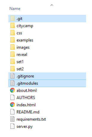
These file components handle all of the version control and tracking as the user commits changes to Git. If the user does not commit their changes to Git, the changes are not “saved” in the version control system. Because of this, it’s best to commit changes at fairly frequent intervals. The committed changes are only active on one particular user’s computer at this point. If the user is working on a branch of another repository, they will want to pull changes from the master repository fairly often to make sure they’re working on the most recent version of the code. If a conflict arises when the branch and the master have both changed in the same place in different ways, the user can work through how to resolve the conflict. When the user wants to integrate their changes with the master repository, the user will create a pull request to the owner of the repository. The owner will then review the changes made and any conflicts that exist, and either choose to accept the pull request to merge the edits into the master repository or send the changes back for additional work. These workflow steps may happen hundreds or thousands of times throughout the lifetime of a code project.
On its own, Git operates off a command line interface; users perform all actions by typing commands. Although this method is perfectly fine, visualizing what’s going on with the project can be a bit hard. To help with that, multiple GUI interfaces have been created to visualize and thus simplify the version control process, and some IDEs include built-in version control hooks. Currently, GitHub is the most popular front-end for Git and offers a free version for basic users.
Resources:
[1] https://en.wikipedia.org/wiki/Version_control
[2] https://github.com/kansasgis/GithubWebinar_2015
[3] https://en.wikipedia.org/wiki/Git
1.8.1 Introduction to Online VCS and GitHub
Introduction to Online VCS
Some popular online hosting solutions for VCS and DVCS code repositories include: GitHub, Bitbucket, Google Code and Microsoft CodePlex. These online repositories are often used as the main trunk repositories for open-source projects with many developers who may be geographically dispersed. For the purposes of this class, we will focus on GitHub.
Introduction to GitHub
GitHub takes all of Git’s version control components, adds a graphical user interface to repositories, change history, and branch documentation, and adds several social components. Users can add comments, submit issues, and get involved in the bug tracking process. Users can follow other GitHub users or specific projects to be notified of project updates. GitHub can either be used entirely online or with an application download for easily managing and syncing local and online repositories. Optional (not required for class): Click here for the desktop application download.
The following exercise will cover the basics of Git and how they’re used in the GitHub website.
Git Exercise in GitHub
- Go to GitHub's website and sign up for an account using any email and password you like. If you already have a GitHub account, feel free to use that.
- Follow the instructions posted at the GitHub Guides Hello World page.
GitHub's change log
GitHub has the ability to display everything that changed with every commit. Take a look at GitHub's Kansasgis/NG911 page. If you click on one of the titles of one of the commits, it displays whatever basic description the developer included of the changes and then as you scroll down, you can see every code change that occurred - red highlighting what was removed and green highlighting what was added. If you mouse over the code, a plus sign graphic shows up, and users can leave comments and such.
Resolving conflicts on GitHub
Conflicts occur if two branches being merged have had different changes in the same places. Git automatically flags conflicts and will not complete the merge like normal; instead, the user will be notified that the conflicts must be resolved. Some conflicts can be resolved inside GitHub, and other types of conflicts have to be resolved in the Git command line [4]. Due to the complexity of resolving conflicts in the command line, it’s best to plan ahead and silo projects as much as possible to avoid conflicts.
Git adds three different markers to the code to flag conflicts:
<<<<<<<HEAD – This marker indicates the beginning of the conflict in the base branch. The code from the base branch is located directly under this marker.
======= – This marker divides the base branch code from the other branch.
>>>>>>> BRANCH-NAME – This marker will have the name of the other branch next to it and indicates the end of the conflict.
Here’s a full example of how Git flags a conflict between branches:
<<<<<<<HEAD
myString = “Monty Python and the Holy Grail is the best. ”
=======
myString = “John Cleese is hilarious.”
>>>>>>> cleese-branch
To resolve the conflict, the user needs to pick what myString will equal. Possible resolution options-
Keeping the base branch -
myString = “Monty Python and the Holy Grail is the best.”
Using the other branch -
myString = “John Cleese is hilarious.”
Combining branches, in this case combining the options -
myString = “Monty Python and the Holy Grail is the best. John Cleese is hilarious.”
GitHub has an interface that can be activated for resolving basic conflicts by clicking on the “Resolve Conflicts” button under the “Pull Requests” tab. This interface steps through each conflict and the user must decide which version to take, keep their changes, use the other changes, or work out a way to integrate both sets of changes. Inside the GitHub interface, the user must also remove the Git symbols for the conflict. The user steps through every conflict in that particular file to decide how to resolve the conflict and then will eventually click on the “Mark as resolved” button. The next file in the project with conflicts will show up and the user will repeat all of the steps until the conflicts are resolved. At this point, the user will click “Commit merge” and then “Merge pull request.”
For more complex types of conflicts like one branch deleting a file that the other keeps, the resolution has to take place in the Git command line. This process can hopefully be avoided, but basic instructions are available at GitHub Help: Resolving a merge conflict using the command line.
Resources:
[4] https://help.github.com/articles/resolving-a-merge-conflict-on-github/
1.8.2 Open source and large companies
GitHub is a great fit for managing open source code projects since, with a free account, all repositories are available on the internet at large. For example, the open source GIS software QGIS (see Lesson 4) is housed on GitHub at GitHub's qgis/QGIS page. Take a look at the repository.
On the front page, you can see in the dashboard statistics that (at the time of this writing) there have been over 40,000 commits, 50 branches, 100 releases, and 250 contributors to the QGIS project. Users worldwide can now contribute their ideas, bugs, and code improvements to a central location that can be managed with standard version control workflows.
Some software companies that have traditionally been protective about their code have adopted GitHub to open certain projects. Esri is rather active on GitHub at GitHub's Esri page including the documentation and samples for the ArcGIS API for Python (see Lesson 3). Microsoft also is present at the GitHub Microsoft page with the tagline “Open source, from Microsoft with love.”
1.8.3 GitHub and Python
While GitHub is open to all digital files and any programming languages, Python is a great fit for use in GitHub for multiple reasons. Unlike other, heavier programming languages, Python doesn’t require extensive libraries with complex dlls and installation structures to get the job done.
Creating Python repositories is as simple as adding the .py files, and then the project can be shared, documented, and updated as needed. GitHub is also a great place to find both Python snippets and entire modules to use. For basic purposes, users can copy/paste just the portions of code off another project they want to try. Otherwise, users can fork an entire repository and tweak it as necessary to fit their purposes.
1.8.4 GitHub's README file
GitHub strongly recommends that every repository contain a README.txt or README.md file. This file will act as the “home page” for the project and is displayed on the repository page after files and folders are listed. This document should contain specific information about the project, how to use it, licensing, and support.
Text files will show up without formatting, so many users choose to use an .md (markdown) file instead. Markdown notation will be interpreted to show various formatting components like font size, bold, italics, imbedded links, numbered lists, and bullet points.
For more information on markdown formatting, visit GitHub Guide's Mastering Markdown page. We will also use Markdown in Lesson 3, in the context of Jupyter notebooks, and provide a brief introduction there.
1.8.5 Gists and GeoJson
Gists
While all free GitHub accounts are required to publish public repositories, all accounts have the ability to create Gists. Gists are single page repositories in GitHub, so they don't support projects with folder structures or multiple files. Since Gists are a single page repository, they are good for storing code snippets or one page projects. Gists can be public or private, even with a free account.
To create a Gist in GitHub, log into GitHub and then click on the plus sign in the upper right hand corner. In the options presented, choose "New gist." Enter a description of the Gist (in figure 1.30 "Delete if Exists Shortcut" is the description) as well as the filename with extension (in figure 1.30 this is DeleteIfExists.py). Enter code or notes in the large portion of the screen or import the code by using the "Add File" button. You have two options for saving your Gist- either "Create secret gist" or "Create public gist."
"Secret" Gists are only mostly secret since they use the internet philosophy of difficult-to-guess urls. If you create a secret Gist, you can still share the Gist with anyone by sending them the url, but there are no logins required to view the Gist. Along this same philosophy, if someone stumbles across the url, they will be able to see the Gist.
For more information about Gists, see the official GitHub documentation at "About Gists" page on Github's website.
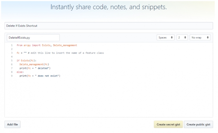
GeoJson
For GIS professionals, Gists are additionally useful since a Gist can be a single GeoJson file. GeoJson files are essentially a text version of geographic data in json formatting. Other developers can instantly access your GeoJson data and incorporate it from GitHub into their online mapping applications without needing to get a hard copy of the shapefile or geodatabase feature class or rely on some kind of map server. GitHub will automatically display GeoJson files as a map whether the file is a Gist or a part of a larger repository. For example, take a look at GitHub's lyzidiamond/learn-geojson page. At first, you’ll see the GeoJson file interpreted as a map. If you click the “Raw” button located on the upper right-ish side of the map, you will see what the GeoJson file looks like in text form. GeoJson can be easily used in Python since after reading in the file, Python can work with the text as if it is one giant dictionary.
1.8.6 GitHub Conclusion
Using GitHub in This Course
In GEOG 489, using GitHub to store the sample code and exercise code from the lessons can be a great way to practice and gain experience with a new software tool. Using GitHub is not required and we don't recommend that you store your completed projects on there. GitHub is an encouraged platform for students to learn since many organizations use GitHub or other VCS.
Conclusion
Git and GitHub provide fast and convenient ways to track projects, whether the project is by one individual or a team of software developers. Although GitHub has many complex features available, it’s easily accessible for individual and small projects that need some kind of tracking mechanism. In addition to version control, GitHub provides users with a social platform for project management as well as the ability for users to create Gists and store GeoJson.
1.9 Investigating IDEs
ArcGIS Pro does install an IDE by default (IDLE which can be accessed from a conda prompt by typing idle) and there is also the straightforward installation of spyder which we covered when we started looking at writing Python 3 code for ArcGIS Pro.
The benefit of using an IDE like spyder is that for more complicated coding and particularly debugging, we have tools that enable us to step through our code line by line, debug and profile multiprocessing code, and watch what is happening in our variables as we saw earlier in the lesson.
While we've had you install and use spyder a little there is a wide range of IDEs that you could use. We’ll provide a brief overview of some different IDEs and code editors in case you would like to use something else (and the choice is entirely yours). Esri supplies a link to a list of IDEs that work with Anaconda (the implementation of conda used for ArcGIS Pro).
Homework Assignment
Part of the homework assignment for this lesson involves selecting an IDE and reviewing it. For full details see the Assignment Page.
Since Python is used in so many different fields and for so many different purposes, there are multiple places Python can be written and edited, and we have seen some of these already.
Some ways are fairly straightforward. You can create a text file, write your Python code, save it with a “.py” extension, and execute it on your computer. However, this approach gives you little to no assistance with writing your code or debugging it.
Because writing code can be such an intensive process, Integrated Development Environment (IDE) applications were developed. Depending on the complexity of the IDE, IDEs can assist developers in a multitude of ways. Many IDEs exist for many different languages, but several focus particularly on Python. Typical Python IDEs include a source code editor and debugging tools. Extended features in some IDEs include
- code auto-completion,
- syntax checking,
- version control,
- environment control,
- and project organization.
IDLE (Python GUI)
IDLE is installed with ArcGIS Desktop software when Python is also installed. IDLE offers very basic code editing capabilities and color codes objects, functions, and methods so users can easily differentiate parts of their code. IDLE also includes a basic debugger that reports messages and errors back to the user. IDLE has some simple text editing tools for bulk indenting, dedenting, commenting, and tabifying.
PythonWin
In GEOG485, we used PythonWin coming with ArcGIS Desktop as the course IDE (until we changed to ArcGIS Pro recently). PythonWin offers a bit more coder assistance and debugging tools than IDLE. For example, the debugger can step through code line by line so you can see exactly what’s going on with your code.
PyScripter
Downloading and Installing
PyScripter is an open-source IDE available for download at SourceForge's PyScripter page. The full project is also available on GitHub at their pyscripter page. Each download of PyScripter installs several different versions of PyScripter so you can select the right one for the version you’re developing in. Developing in the wrong version of Python can lead to compatibility issues and lost functionality.
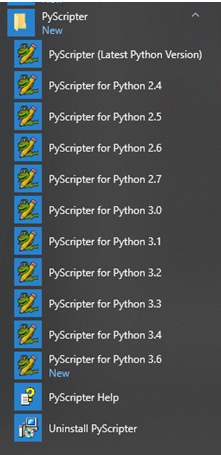
If you want to use PyScripter to develop code to be used in ArcGIS Desktop software, you will want to know ahead of time that ArcGIS Desktop uses Python 2.7 and that ArcGIS Desktop is a 32-bit software program. On SourceForge, the PyScripter version is not related to any Python version, so you’ll probably just want to download the latest version of PyScripter without the term “x64” included in it. As you can see in Figure 1.31, this installation of PyScripter will include versions for Python 2.4 through 3.6. For ArcGIS Desktop, you’ll want to use PyScripter for Python 2.7.
If you want to use PyScripter to develop for ArcGIS Pro or to use the ArcGIS API for Python, you’ll want to download and install the latest version that includes “x64.” To check and see what version of Python ArcGIS Pro is using, open ArcGIS Pro, and on the “Analysis” tab, open the Python interpreter. Inside the Python interpreter, type in the following lines:
import sys
sys.version_info
The Python window will report back what version of Python ArcGIS Pro is using so you can use the corresponding PyScripter version. In Figure 1.32, the version used is 3.5.3, so PyScripter for Python 3.5 would be used.
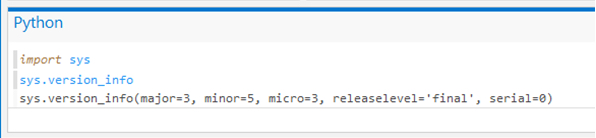
Using PyScripter
PyScripter has many tools available for making developer’s lives easier. The source code editor includes auto-completion and a built-in syntax checker. Each developer can also customize certain parts of the interface based on their personal preferences. PyScripter also has more advanced debugging tools than IDLE or PythonWin.
PyCharm
PyCharm is another popular IDE that has a free community edition available to download- see the Jet Brains Download PyCharm page. PyCharm differs from PyScripter the most in that PyCharm integrates easily with conda, so developers can specify which conda environment a project needs to be developed in and run on. PyCharm has many different development aids and tools available including auto-completion, enhanced debugging, various integrated code-checking processes, error detection, and on-the-fly code fixes.
Python Tools for Visual Studio
Microsoft has a plugin for Visual Studio so it can be used as a Python IDE. Visual Studio has Community Editions available for free download, and Python Tools for Visual Studio can be downloaded and installed- see Microsoft's How to Install Python Support in Visual Studio on Windows page. For Visual Studio 2015 and lower, you must also install a Python interpreter. Visual Studio is a robust IDE with organization tools that can integrate project components from various source code languages as well as auto-completion and enhanced debugging. Visual Studio can also be used to directly debug certain Python components in ArcGIS Pro including script tool execution, tool validation, and Python toolboxes.
Others
There are multiple other Python IDEs available, and what to pick usually depends on a developer’s personal preference. Others include Eclipse/PyDev, Eric, and Spyder of course.
For more information about IDEs in general, feel free to refer to these links: Wikipedia's page for Integrated Development Environment, Esri's Technical Support Page, and ArcGIS Pro's Debug Python code page.
Lesson 1 Homework Assignment
Part 1- IDE Research (25% of Project 1 score)
For the first part of the Lesson 1 homework project, you will be evaluating an IDE. Each student will be evaluating a different IDE and can “claim” their IDE in the "L1: IDE Investigation: Choose topic" discussion forum within Canvas. Possible IDEs include but are not limited to the following (please do NOT choose Spyder!):
- PyScripter
- PyCharm
- Visual Studio with Python plugin
- Eric
- PyDev
- Wing
- Notepad++ with Python plugin
Part I Deliverable
First, claim your IDE in the "L1: IDE Investigation: Choose topic" discussion forum. Then experiment with writing and debugging code in that IDE and study the documentation. Pay special attention to which of the features mentioned in Section 1.9 (auto-completion, syntax checking, version control, environment control, and project organization) are available in that IDE. Record a 5 minute demo and discussion video of your chosen IDE using Kaltura that highlights the IDE’s features, functionalities, and possible difficulties. Post a link to your video in the Media Gallery.
Part 2 – Python coding and profiling (75% of Project 1 score)
We are going to use the arcpy vector data processing code from Section 1.6.6.2 (download Lesson1_Assignment_initial_code.py) as the basis for our Lesson 1 programming project. The code is already in multiprocessing mode, so you will not have to write multiprocessing code on your own from scratch but you still will need a good understanding of how the script works. If you are unclear about anything the script does, please ask on the course forums. This part of the assignment will be for getting back into the rhythm of writing arcpy based Python code and practice creating script tool with ArcGIS Pro. Your task is to extend our vector data clipping script by doing the following:
- Modify the code to handle a parameterized output folder path (still using unique output filenames for each shapefile) defined in a third input variable at the beginning of the main script file. One way to achieve this task is by adding another (5th) parameter to the worker() function to pass the output folder information along with the other data.
- Implement and run simple code profiling using the time module as in Section 1.6 and then perform basic profiling in spyder as we did in Section 1.7.2.1 (no visual or line profiling needed). You won't be able to get profiling results for the subprocesses running the worker() function from this but you should report the total time and the computation times you get for the main functions from scriptool.py involved in your write-up and explain where the most time has been spent. Also include a screenshot showing the profiling results in spyder.
- Create an ArcGIS Pro script tool for running the modified code. The script tool should have three parameters allowing the user to provide the clipper feature class, the to-be-clipped feature class, and the output folder.
- Expand the code so that it can handle multiple input feature classes to be clipped (still using a single polygon clipping feature class). The input variable tobeclipped should now take a list of feature class names rather than a single name. The worker function should, as before, perform the operation of clipping a single input file (not all of them!) to one of the features from the clipper feature class. The main change you will have to make will be in the main code where the jobs are created. The names of the output files produced should have the format
clip_<oid>_<name of the input feature class>.shp
, so for instance clip_0_Roads.shp for clipping the Roads feature class from USA.gdb to the state with oid 0. Do this after the profiling stage and you do not need to run profiling for this nor create a script tool for this modified version, so you may want to replace the calls of GetParamterAsText() by hardcoded paths again. - Successful delivery of the above requirements is sufficient to earn 90% on the project. The remaining 10% is reserved for efforts that go "over and above" the minimum requirements. Over and above points may be earned by sharing your profiling results only (not the code and not the other parts of your write-up!) by uploading them to GitHub, adding in-tool documentation, creating a script tool for the multiple-input-files version from step (4), adding further geoprocessing operations (e.g. reprojection) to the worker() function, or other enhancements as you see fit. You can also try to improve the efficiency of the code based on the profiling results.
You will have to submit several versions of the modified script for this assignment:
- (A) The modified single-input-file script tool version from step (3) above together with the .tbx file for your toolbox.
- (B) The multiple-input-files version from step (4).
- (C) Potentially a third version if you made substantial modifications to the code for "over and above" points (step (5) above). If you created a new script tool for this, make sure to include the .tbx file as well.
To realize the modified code versions in this assignment, all main modifications have to be made to the input variables and within the code of the worker() and mp_handler() functions; the code from the get_install_path() function should be left unchanged. Of course, we will also look at code quality, so make sure the code is readable and well documented. Here are a few more hints that may be helpful:
Hint 1:
When you adapt the worker() function, I strongly recommend that you do some tests with individual calls of that function first before you run the full multiprocessing version. For this, you can, for instance, comment out the pool code and instead call worker() directly from the loop that produces the job list, meaning all calls will be made sequentially rather than in parallel. This makes it easier to detect errors compared to running everything in multiprocessing mode right away. Similarly, it could be a good idea to add print statements for printing out the parameter tuples placed in the job list to make sure that the correct values will be passed to the worker function.
Hint 2 (concerns step (4)):
When changing to the multiple-input-files version, you will not only have to change the code that produces the name of the output files in variable outFC by incorporating the name of the input feature class, you will have to do the same for the name of the temporary layer that is being created by MakeFeatureClass_managment() to make sure that the layer names remain unique. Else some worker calls will fail because they try to create a layer with a name that is already in use.
To get the basename of a feature class without file extension, you can use a combination of the os.path.basename() and os.path.splitext() functions defined in the os module of the Python standard library. The basename() function will remove the leading path (so e.g., turn "C:\489\data\Roads.shp" into just "Roads.shp"). The expression os.path.splitext(filename)[0] will give you the filename without file extension. So for instance "Roads.shp" will become just "Roads". (Using [1] instead of [0] will give you just the file extension but you won't need this here.)
Hint 3 (concerns steps (4) and (5)):
This is not required but if you decide to create a script tool for the multiple-input-files version from step (4) for over and above points, you will have to use the "Multiple value" option for the input parameter you create for the to-be-clipped feature class list in the script tool interface. If you then use GetParameterAsText(...) for this parameter in your code, what you will get is a single string(!) with the names of the feature classes the user picked separated by semicolons, not a list of name strings. You can then either use the string method split(...) to turn this string into a list of feature class names or you use GetParameter(...) instead of GetParameterAsText(...) which will directly give you the feature class names as a list.
Part 2 Deliverable
Submit a single .zip file to the corresponding drop box on Canvas; the zip file should contain:
- Your modified code files and ArcGIS Pro toolbox files (up to three different versions as described above). Please organize the files cleanly, e.g., using a separate subfolder for each version.
- A 400-word write-up of what you have learned during this exercise. This write-up should also include your profiling results and insights (including the spyder profiling screenshot) and a description of what you did for "over and above" points (if anything). In addition, think back to the beginning of Section 1.6.6 and include a brief discussion of any changes to the processing workflow and/or the code that might be necessary if we wanted to write our output data to geodatabases and briefly comment on possible issues (using pseudocode or a simple flowchart if you wish).
Lesson 2 GUI Development with PyQt5 and Package Management
2.1 Overview and Checklist
Lesson 2 is two weeks in length. We will look at some more advanced Python concepts and how to access data on the web from within a Python program. Then we will focus on how write Python programs with a graphical user interface based on the QT5 library and PyQt5 package. Finally, we will discuss Python package management and package managers, and how they can be used to disseminate Python code.
Please refer to the Calendar for specific time frames and due dates. To finish this lesson, you must complete the activities listed below. You may find it useful to print this page out first so that you can follow along with the directions.
| Step | Activity | Access/Directions |
|---|---|---|
| 1 | Engage with Lesson 2 Content | Begin with 2.2 List Comprehension |
| 2 | Programming Assignment and Reflection | Submit your code for the programming assignment and 400 words write-up with reflections |
| 3 | Quiz 2 | Complete the Lesson 2 Quiz |
| 4 | Questions/Comments | Remember to visit the Lesson 2 Discussion Forum to post/answer any questions or comments pertaining to Lesson 2 |
2.2 List comprehension
Like the first lesson, we are going to start Lesson 2 with a bit of Python theory. From mathematics, you probably are familiar with the elegant way of defining sets based on other sets using a compact notation as in the example below:
M = { 1, 5 ,9, 27, 31}
N = {x2, x ∈ M ∧ x > 11}
What is being said here is that the set N should contain the squares of all numbers in set M that are larger than 11. The notation uses { … } to indicate that we are defining a set, then an expression that describes the elements of the set based on some variable (x2) followed by a set of criteria specifying the values that this variable (x) can take (x ∈ M and x > 11).
This kind of compact notation has been adopted by Python for defining lists and it is called list comprehension. A list comprehension has the general form
[< new value expression using variable> for <variable> in <list> if <condition for variable>]
The fixed parts are written in bold here, while the parts that need to be replaced by some expressions using some variable are put into angular brackets <..> . The if and following condition are optional. To give a first example, here is how this notation can be used to create a list containing the squares of the numbers from 1 to 10:
squares = [ x**2 for x in range(1,11) ]
print(squares)
Output:
[1, 4, 9, 16, 25, 36, 49, 64, 81, 100]
In case you haven’t seen this before, ** is the Python operator for a to the power of b.
What happens when Python evaluates this list comprehension is that it goes through the numbers in the list produced by range(1,11), so the numbers from 1 to 10, and then evaluates the expression x**2 with each of these numbers assigned to variable x. The results are collected to form the new list produced by the entire list comprehension. We can easily extend this example to only include the squares of numbers that are even:
evenNumbersSquared = [ x**2 for x in range(1,11) if x % 2 == 0 ]
print(evenNumbersSquared)
Output:
[4, 16, 36, 64, 100]
This example makes use of the optional if condition to make sure that the new value expression is only evaluated for certain elements from the original list, namely those for which the remainder of the division by 2 with the Python modulo operator % is zero. To show that this not only works with numbers, here is an example in which we use list comprehension to simply reduce a list of names to those names that start with the letter ‘M’ or the letter ‘N’:
names = [ 'Monica', 'John', 'Anne', 'Mike', 'Nancy', 'Peter', 'Frank', 'Mary' ]
namesFiltered = [ n for n in names if n.startswith('M') or n.startswith('N') ]
print(namesFiltered)
Output:
['Monica', 'Mike', 'Nancy', 'Mary']
This time, the original list is defined before the actual list comprehension rather than inside it as in the previous examples. We are also using a different variable name here (n) so that you can see that you can choose any name here but, of course, you need to use that variable name consistently directly after the for and in the condition following the if. The new value expression is simply n because we want to keep those elements from the original list that satisfy the condition unchanged. In the if condition, we use the string method startswith(…) twice connected by the logical or operator to check whether the respective name starts with letter ‘M’ or the letter ‘N’.
Surely, you are getting the general idea and how list comprehension provides a compact and elegant way to produce new lists from other lists by (a) applying the same operation to the elements of the original list and (b) optionally using a condition to filter the elements from the original list before this happens. The new value expression can be arbitrarily complex involving multiple operators as well as function calls. It is also possible to use several variables, either with each variable having its own list to iterate through corresponding to nested for-loops, or with a list of tuples as in the following example:
pairs = [ (21,23), (12,3), (3,11) ]
sums = [ x + y for x,y in pairs ]
print(sums)
Output:

[44, 15, 14]
With “for x,y in pairs” we here go through the list of pairs and for each pair, x will be assigned the first element of that pair and y the second element. Then these two variables will be added together based on the expression x + y and the result will become part of the new list. Often we find this form of a list comprehension used together with the zip(…) function from the Python standard library that takes two lists as parameters and turns them into a list of pairs. Let’s say we want to create a list that consists of the pairwise sums of corresponding elements from two input lists. We can do that as follows:
list1 = [ 1, 4, 32, 11 ]
list2 = [ 3, 2, 1, 99 ]

sums = [ x + y for x,y in zip(list1,list2) ]
print(sums)
Output:
[4, 6, 33, 110]
The expression zip(list1,list2) will produce the list of pairs [ (1,3), (4,2), (32,1), (11,99) ] from the two input lists and then the rest works in the same way as in the previous example.
Most of the examples of list comprehensions that you will encounter in the rest of this course will be rather simple and similar to the examples you saw in this section. We will also practice writing list comprehensions a bit in the practice exercises of this lesson. If you'd like to read more about them and see further examples, there are a lot of good tutorials and blogs out there on the web if you search for Python + list comprehension, like this List Comprehensions in Python page for example. As a last comment, we focussed on list comprehension in this section but the same technique can also be applied to other Python containers such as dictionaries, for example. If you want to see some examples, check out the section on "Dictionary Comprehension" in this article here.
2.3 Accessing and working with web data
There is a wealth of geographic (and other) information available out there on the web in the form of web pages and web services, and sometimes we may want to make use of this information in our Python programs. In the first walkthrough of this lesson, we will access two web services from our Python code that allow us to retrieve information about places based on the places’ names. Another common web-based programming task is scraping the content of web pages with the goal of extracting certain pieces of information from them, for instance links leading to other pages. In this section, we are laying the foundation to perform such tasks in Python by showing some examples of working with URLs and web requests using the urllib and requests packages from the standard Python library, and the BeautifulSoup4 (bs4) package, which is a 3rd party package that you will have to install.
Urllib in Python 3 consists of the three main modules urllib.requests for opening and reading URLs, urllib.error defining the exceptions that can be raised, and urllib.parse for parsing URLs. It is quite comprehensive and includes many useful auxiliary functions for working with URLs and communicating with web servers, mainly via the HTTP protocol. Nevertheless, we will only use it to access a web page in this first example here, and then we will switch over to using the requests package instead, which is more convenient to use for the high-level tasks we are going to perform.
In the following example, we use urllib to download the start page from Lesson 1 of this course:
import urllib.request

url = "https://www.e-education.psu.edu/geog489/l1.html"
response = urllib.request.urlopen(url)
htmlCode = response.read()
print(htmlCode)
After importing the urllib.request module, we define the URL of the page we want to access in a string variable. Then in line 4, we use function urlopen(…) of urllib to send out an HTTP request over the internet to get the page whose URL we provide as a parameter. After a successful request, the response object returned by the function will contain the html code of the page and we can access it via the read() method (line 5). If you run this example, you will see that the print statement in the last line prints out the raw html code of the Lesson 1 start page.
Here is how the same example looks using the requests package rather than urllib:
import requests

url = "https://www.e-education.psu.edu/geog489/l1.html"
response = requests.get(url)
htmlCode = response.text
print(htmlCode)
As you can see, for this simple example there really isn’t a big difference in the code. The function used to request the page in line 4 is called get(…) in requests and the raw html code can be accessed by using a property called text of the response object in line 5 not a method, that’s why there are no parentheses after text.
The most common things returned by a single web request, at least in our domain, are:
- html code
- plain text
- an image (e.g. JPEG or PNG)
- XML code
- JSON code
Most likely you are at least somewhat familiar with html code and how it uses tags to hierarchically organize the content of a page including semantic and meta information about the content as well as formatting instructions. Most common browsers like Chrome, Firefox, and Edge have some tools to inspect the html code of a page in the browser. Open the first lesson page in a new browser window and then do a right-click -> Inspect (element) on the first bullet point for “1.1 Overview and Checklist” in the middle of the window. That should open up a window in your browser showing the html code with the part that produces this line with the link to the Section 1.1 web page highlighted as in the figure below.
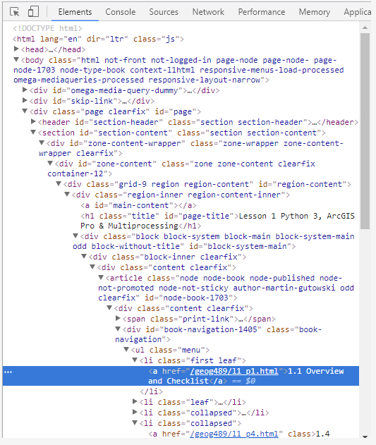
The arrows indicate the hierarchical organization of the html code, the so-called Document Object Model (DOM), and can be used to unfold/fold in part of the code. Also note how most html tags (‘body’,‘div’, ‘a’, ‘span’, etc.) have an attribute “id” that defines a unique ID for that element in the document as well as an attribute “class” which declares the element to be of one or several classes (separated by spaces) that, for instance, affect how the element will be formatted. We cannot provide an introduction to html and DOM here but this should be enough background information to understand the following examples. (These topics are addressed in more detail in our GEOG 863 class.)
Unless our program contains a browser component for displaying web pages, we are typically downloading the html code of a web page because we are looking for very specific information in that code. For this, it is helpful to first parse the entire html code and create a hierarchical data structure from it that reflects the DOM structure of the html code and can be used to query for specific html elements in the structure to then access their attributes or content. This is exactly what BeautifulSoup does.
Go ahead and install the beautifulsoup4 package in the Python Package Manager of ArcGIS Pro as you did with Spyder in Section 1.5. Once installed, BeautifulSoup will be available under the module name bs4. The following example shows how we can use it to access the <title> element of the html document:
import requests
from bs4 import BeautifulSoup

url = "https://www.e-education.psu.edu/geog489/l1.html"
response = requests.get(url)
soup = BeautifulSoup(response.text, 'html.parser')

print(soup.find('title'))
Output:
<title>Lesson 1 Python 3, ArcGIS Pro & Multiprocessing | GEOG 489: GIS Application Development</title>
In line 6, we are taking the raw html code from response.text and create a BeautifulSoup object from it using an html parser and store it in variable soup. Parsing the html code and creating the hierarchical data structure can take a few seconds. We then call the find(…) method to get the element demarcated by the title tags <title>…</title> in the document. This works fine here for <title> because an html document only contains a single <title> tag. If used with other tags, find(…) will always return only the first element, which may not be the one we are looking for.
However, we can provide additional attributes like a class or id for the element we are looking for. For instance, the following command can be used to get the link element (= html tag <a>) that is of the class “print-page”:
print(soup.find('a', attrs = {'class': 'print-page'}))
The output will start with <a class=”print-page” href…” and include the html code for all child elements of this <a> element. The “attrs” keyword argument takes a dictionary that maps attribute names to expected values. If we don’t want to print out all this html code but just a particular attribute of the found element, we can use the get(…) method of the object returned by find(…), for instance with ‘href’ for the attribute that contains the actual link URL:
element = soup.find('a', attrs = {'class': 'print-page'})
print(element.get('href'))
Output:
https://www.e-education.psu.edu/geog489/print/book/export/html/1703
You can also get a list of all elements that match the given criteria, not only the first element, by using the method find_all(…) instead of find(…). But let’s instead look at another method that is even more powerful, the method called select(…). Let’s say what we really want to achieve with our code is extract the link URLs for all the pages linked to from the content list on the page. If you look at the highlighted part in the image above again, you will see that the <a> tags for these links do not have an id or class attribute to distinguish them from other <a> tags appearing in the document. How can we unambiguously characterize these links?
What we can say is that these are the links that are formed by a <a> tag within a <li> element within a <ul> element within a <div> element that has the class “book-navigation”. This condition is only satisfied by the links we are interested in. With select(…) we can perform such queries by providing a string that describes these parent-child relationships:
elementList = soup.select('div.book-navigation > ul > li > a')
for e in elementList:
	print(e.get('href'))
Output:
/geog/489/l1_p1.html
/geog/489/l1_p2.html
/geog/489/l1_p3.html
…
The list produced by the code should consist of ten URLs in total. Note how in the string given to select(…) the required class for the <div> element is appended with a dot and how the > symbol is used to describe the parent-child relationships along the chain of elements down to the <a> elements we are interested in. The result is a list of elements that match this condition and we loop through that list in line 2 and print out the “href” attribute of each element to display the URLs.
One final example showing the power of BeautifulSoup: The web page www.timeanddate.com, among other things, allows you to look up the current time for a given place name by directly incorporating country and place name into the URL, e.g.
http://www.timeanddate.com/worldclock/usa/state-college
… to get a web page showing the current time in State College, PA. Check out the web page returned by this request and use right-click -> Inspect (element) again to check how the digital clock with the current time for State College is produced in the html code. The highlighted line contains a <span> tag with the id “ct”. That makes it easy to extract this information with the help of BeautifulSoup. Here is the full code for this:
import requests
from bs4 import BeautifulSoup

url = "http://www.timeanddate.com/worldclock/usa/state-college"

response = requests.get(url)
soup = BeautifulSoup(response.text, 'html.parser')
time = soup.find('span', attrs= { 'id': 'ct'})

print('Current time in State College: ' + time.text)
Output:
Current time in State College: 13:32:28
Obviously, the exact output depends on the time of day you run the code. Please note that in the last line we use time.text to get the content of the <span> tag found, which is what appears between the <span> and </span> tags in the html.
We are intentionally only doing this for a single place here because if you ever do this kind of scraping of web pages on a larger scale, you should make sure that this form of usage is not against the web site’s terms of use. In addition, some things can be done to keep the load on the server produced by web scraping as low as possible, e.g. by making sure the results are stored/cached when the program is running and not constantly being queried again unless the result may have changed. In this example, while the time changes constantly, one could still only run the query once, calculate the offset to the local computer’s current time once, and then always recalculate the current time for State College based on this information and the current local time.
The examples we have seen so far all used simple URLs, although this last example was already an example where parameters of the query are encoded in the URL (country and place name), and the response was always an html page intended to be displayed in a browser. In addition, there exist web APIs that realize a form of programming interface that can be used via URLs and HTTP requests. Such web APIs are, for instance, available by Twitter to search within recent tweets, by Google Maps, and by Esri. Often there is a business model behind these APIs that requires license fees and some form of authorization.
Web APIs often allow for providing additional parameters for a particular request that have to be included in the URL. This works very similar to a function call, just the syntax is a bit different with the special symbol ? used to separate the base URL of a particular web API call from its parameters and the special symbol & used to separate different parameters. Here is an example of using a URL for querying the Google Books API for the query parameter “Zandbergen Python”:
https://www.googleapis.com/books/v1/volumes?q=Zandbergen%20Python
www.googleapis.com/books/v1/volumes is the base URL for using the web API to perform this kind of query and q=Zandbergen%20Python is the query parameter specifying what terms we want to search for. The %20 encodes a single space in a URL. If there would be more parameters, they would be separated by & symbols like this:
<parameter 1>=<value 1>&<parameter 2>=<value 2>&…
We also mentioned above that one common response format is JSON (JavaScript Object Notation) code. If you actually click the link above, you will see that Google sends back the response as JSON code. JSON is intended to be easily readable by computers not humans, but the good thing is that we as Python programmers are already used to reading it because it is based on notations for arrays (=lists) and objects (=dictionaries) that use the same syntax as Python.
Study the JSON response to our Zandbergen query from above for a moment. At the top level we have a dictionary that describes the response. One entry “totalItems” in the dictionary says that the response contains 16 results. The entry “items” contains these results as a list of dictionaries/objects. The first dictionary from the list is the one for our course textbook. One attribute of this dictionary is “volumeInfo”, which is again a dictionary/object whose attributes include the title of the book and name of the author. Please note that the “authors” attribute is again a list because books can have multiple authors. If you scroll down a bit, you will see that at some point the dictionary for the Zandbergen book is closed with a “}” and then a new dictionary for another book starts which is the second item from the “items” list, and so on.
After this explanation of web APIs and JSON, here is the Python code to run this query and process the returned JSON code:
import requests, urllib.parse

url = "https://www.googleapis.com/books/v1/volumes"
query = "Zandbergen Python"

parameterString = "?q=" + urllib.parse.quote(query)

response = requests.get(url + parameterString)
jsonCode = response.json()

print(jsonCode['items'][0]['volumeInfo']['title'])
Output:
Python Scripting for Arcgis
We here define the base URL for this web API call and the query term string in different variables (lines 3 and 4). You saw above that certain characters like spaces appearing in URLs need to be encoded in certain ways. When we enter such URLs into a browser, the browser will take care of this but if we construct the URL for a request in our code we have to take care of this ourselves. Fortunately, the urllib.parse module provides the function quote(…) for this, which we use in line 6 to construct the correctly encoded parameter list which is then combined with the base url in the call of requests.get(…) in line 8.
By using the json() method of the response object in line 9, we get a Python data structure that will represent the JSON response and store it in variable jsonCode. In this case, it is a dictionary that under the key “items” contains a Python list with dictionaries for the individual book items returned. In line 11, we use this data structure to access the 'title' attribute of the first book item in the list: With ['items'] we first get the “items” list, then we take the first element from that list with [0], then we access the 'volumeInfo' property of the resulting dictionary, and finally with ['title'] we get the 'title' attribute from the volume info dictionary.
The code from above was supposed to show you how you to explicitly encode parameters for web API requests (with the help of urllib.parse.quote(...)) and build the final URL. The great thing about the requests module is that it can take care of all these things for you: You can simply provide an additional parameter for get(…) that contains a dictionary of parameter names for the web request and what values should be assigned to these parameters. Requests then automatically encodes these values and builds the final URL. Here is the version of the previous example that uses this approach.
import requests

url = "https://www.googleapis.com/books/v1/volumes"
query = "Zandbergen Python"

response = requests.get(url, {'q': query})
jsonCode = response.json()

print(jsonCode['items'][0]['volumeInfo']['title'])
The dictionary with parameters for the web request that we use in line 6 says that the value assigned to parameter 'q' should be the string contained in variable query. As said, requests will automatically take care of encoding special characters like spaces in the parameter values and of producing the final URL from them.
You will see more examples of using web APIs and processing the JSON code returned in the first walkthrough of this lesson. These examples will actually return GeoJSON code which is a standardized approach for encoding spatial features in JSON including their geometry data. However, there is a rather large but also very interesting topic that we have to cover first.
2.4 GUI programming basics
By now you probably already have a very good idea of how one can write longer and more complex Python programs including standalone programs that work outside of the ArcGIS script tool environment (for example running code from the command prompt or IPython). Functions and modules are two of the main constructs for splitting the code into smaller units and keeping it readable, manageable, and reusable. However, there is one key component of standalone programs that we have not really discussed in GEOG485 and this course so far, and that is the design and creation of graphical user interfaces (GUIs) for your Python programs. These days we are all used to working with a mouse or other pointing device to interact with the different windows, buttons, and other interactive elements that make up the GUI of most of the software applications we are using. Maybe you have already wondered about how to create such GUI-based software with Python.
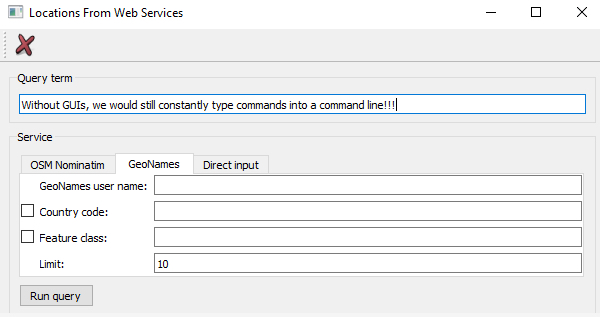
When writing script tools for ArcGIS, we mainly relied on the script tool dialog box provided by ArcGIS for a GUI that allows the user to provide values for the input variables of our script tool in a convenient way. In our Python code, we didn’t have to worry about the dialog box; this was all automatically taken care of by ArcGIS based on the parameters we declared for our script tool. However, even in the context of more advanced script tools, being able to create and use your own GUIs in Python can be very useful, for instance when you want to create a script tool that requires a lot of interaction with the user and additional input while the tool is being executed (an example of such a tool will be discussed later in this lesson). Therefore, it is really getting time for us to talk a bit about GUI development in general, and in Python in particular!
To create a GUI in a given programming language and for a given platform, you often can choose between different GUI libraries (also called GUI toolkits) available for that language and platform. These GUI libraries define classes and auxiliary functions that allow for creating, combining, connecting, and managing the different components of a GUI such as windows, buttons, etc. with a minimal amount of code. Often, GUI libraries are also simply referred to as GUIs, so the term can either mean a particular software library or package used for creating graphical interfaces or the concrete interface created for a particular application. Moreover, some libraries contain much more than just the GUI related classes and components. For instance, the QT5 library we are going to talk about and use later on is actually a cross-platform application development framework with support for non-GUI related things like database and network access.
A GUI library is often complemented by additional tools for supporting the creation of graphical interfaces with that library. Some languages provide a GUI library as part of their standard library, so it is directly available on all platforms the language is available for without having to install additional 3rd party packages. There also exist GUI libraries that have been made available for different languages like the already mentioned QT library that is written in C++ but can be used with a large number of different programming languages. Wrapper packages, also called bindings, make the components and functionality of the library available in the respective other programming language. In the case of QT, there exist two commonly used wrapper packages for Python, PyQT and PySide (see Section 2.5.2.1). In the following, we provide a brief overview on the main concepts and techniques related to GUI development that we encounter in most GUI libraries.
2.4.1 GUI widgets
We already mentioned some of the main visible components that serve as the construction blocks for building GUIs in typical GUI libraries, like windows and buttons. The image below shows a few more that we commonly encounter in today’s software applications including group boxes, labels, check boxes, radio buttons, combo boxes, line input fields, text input areas, tab views, and list views. Others that you are probably familiar with are tool bars, tool buttons, menu bars, context menus, status bars, and there are many, many more!

Typically, the GUI library contains classes for each of these visible elements, and they are often referred to as the widgets. Certain widgets can serve as containers for other widgets and, as a result, widgets tend to be organized hierarchically within a concrete graphical interface. For instance, a dialog box widget can contain many other widgets including a tab widget that in turn contains labels and buttons on each of its tab areas. If a widget A directly contains another widget B, we say that B is a child of A and A is B’s parent. A widget without a parent is a window that will be displayed independently on the screen. Widgets can have many different attributes for controlling their visual appearance, their layout behavior, and how they operate. Methods defined in the respective widget class allow for accessing and modifying these attributes. The most common operations performed with widgets in program code are:
- Creating the widget
- Adding the widget to another widget (widget becomes the child of that other widget)
- Adding another widget to the widget (the widget becomes the parent containing the other widget)
- Changing an attribute of the widget (for instance, you may change the text displayed by a label widget)
- Reading an attribute of the widget (for instance, you may need to get the text that a user entered into a line input widget)
- Setting the layout management method for the widget; this determines how the child widgets of that widget will be arranged to fill the widget’s content area
- Linking an event that the widget can trigger to event handler code that should be executed in that case (for instance, you may want that a particular function in your code be called when a particular button is clicked)
We will explain the ideas of layout management and event handling hinted at in the last two bullet points above in more detail in the next sections. From the user's perspective, widgets can be interacted with in many different ways depending on the type of the widget, including the following very common forms of interactions:
- The user can click on the widget with the mouse to start some action, change the state of the widget, or open a context menu.
- The user can give focus to a widget either by clicking it or using the TAB key for moving the focus to the next widget in a specified order. At any time, only a single widget can have focus, meaning it will receive keyboard input which allows for typing into a text input widget or "clicking" a button by pressing ENTER. Similarly, the user makes a widget lose focus when giving focus to another widget.
- The user can enter some text into the widget.
- The user can drag the widget and drop it onto another widget, or drop something on the widget.
In addition, there are complex widgets that allow the user to interact with them and change their state by clicking on particular parts of a widget. Examples are the user unfolding a combo box to select a different value, the user clicking on a menu in the menu bar to open that menu and select an item in it, the user moving the slider component of a widget to adapt some value, or the user selecting a color by clicking on a particular location in a widget with a chromatic circle. The events caused by such user interactions are what drives the order of code execution in the underlying program code as will be further explained in Section 2.4.3.
2.4.2 Layout management
Widgets can be freely arranged within the content area of their parent widget (for instance a window widget). This can be done with the help of pixel coordinates that are typically measured from the top left corner of the content area. However, it would be very cumbersome to create GUIs by specifying the x and y coordinates and width and height values for each widget. More importantly, such a static layout will only look good for the particular size of the parent it has been designed for. When the containing window is resized by the user, you would expect that the dimensions and positions of the contained widgets adapt accordingly which will not be the case for such a static coordinate-based layout.
Therefore, in modern GUI libraries the task of arranging the child widgets within the parent widget is taken care of by so-called layout managers. This happens dynamically, so if the window is resized, all content will be rearranged again down the hierarchy of widgets by the different layout managers involved. The GUI library defines different layout classes to create the layout manager objects from. The three most common layout types are:
- Horizontal layout: All child widgets are arranged horizontally in the order in which they have been added to the parent
- Vertical layout: All child widgets are arranged vertically in the order in which they have been added to the parent
- Grid layout: Child widgets are arranged in a table or grid layout consisting of columns and rows. The child widgets are added to a particular cell in the layout by providing row and column indices and can potentially span multiple rows and/or columns.
The images below illustrate these three basic layout types for a set of three label and three push button widgets. Because of their layout preferences, both labels and buttons remain at their preferred height in the horizontal layout, but are expanded to fill the available space horizontally in the vertical layout. In the grid layout, the labels have been set up to form the first column of a grid with 3 rows and 2 columns, while the buttons have been set up to occupy the cells in the second column.
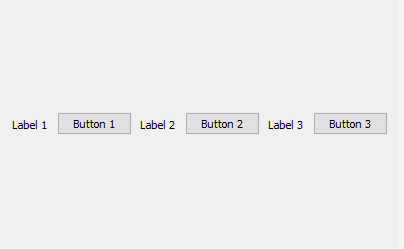
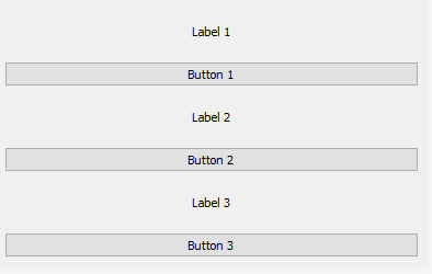
In many cases, these three layout types are already sufficient to arrange the widgets as desired because of the way layouts can be nested. For instance, you can have the components of a window organized in a grid layout and then use a vertical layout to arrange several widgets within one of the cells of the grid. As indicated above, widgets have attributes that affect their layout behavior and, as a result, how much space the layout manager will assign to them in the vertical and horizontal dimensions taking into account the other child widgets of the same parent and their attributes. These attributes can, for instance, define the minimum, preferred, and/or maximum dimensions or general size policies for width and height. For instance, as we saw in the examples from the previous figures, a standard push button widget often has a size policy for its height that says that the height should not be increased beyond its default height even if there is space available, while in the horizontal dimension the button may be expanded to fill available space that the layout manager would like to fill. We will talk more about layout management when we will start to work with the QT library later on in this lesson.
2.4.3 Events and event handling, signals and slots
So far, we are used to the code in a script file being executed line-by-line from the top to the bottom with the order of execution only being affected by loops, if-else and function calls. GUI based applications operate a bit differently. They use what is called an event-driven programming approach. In event-driven programming, the code is organized as follows:
- Initalization phase:
- The GUI is created by instantiating the widgets (= creating objects of the widget classes) and organizing them in parent-child hierarchies using suitable layout manager objects to achieve the desired arrangement.
- Event handling code is defined for dealing with events from user interactions (like clicking a button) or other types of events.
- Different events are associated with the corresponding event handling code.
- Execution phase:
- An infinite loop is started that waits for GUI events and only terminates if the application is closed. In the loop, whenever an event occurs, the respective event handling code is executed, then the waiting continues until the next event happens.
The order of the first two points of the initialization phase can sometimes be swapped. The code for running the event processing loop is something you do not have to worry about when programming GUI based applications because that part is being taken care of by the GUI library code. You just have to add a command to start the loop and be aware that this is happening in the background. Your main job is to produce the code for creating the GUI and defining the event handlers in the initialization part of the program.
As indicated above, widgets can be interacted with in different ways and such interactions cause certain types of events that can be reacted on in the code. For instance, a button widget may cause a “button pressed” event when the user presses the left mouse button while having the mouse cursor over that button and a “button released” event when the mouse button is released again. In addition, it will cause a “button triggered” event after the release but this event can also be triggered by pressing the RETURN key, while the button has focus (e.g. when the button is hovered over with the mouse). The functionality of the GUI is realized by setting up the event handler code. That code typically consists of the definitions of event handler functions that are invoked when a certain event is caused and that contain the code that determines what should happen in this case. For instance, we may set up an event handler function for the “button triggered” event of the mentioned button. The code of that function may, for example, open a dialog box to get further information from the user or start some computations followed by displaying the results.
Precisely how events are linked to event handling functions depends on the GUI library used. We will see quite a few examples of this later in this lesson. However, we already want to mention that in the QT library we are going to use, the event-based approach is covered under what QT calls the signals & slots approach. When an event occurs for a particular QT widget (e.g., user clicks button), that widget emits a signal specific for that event. A slot is a function that can be called in response to a signal (so essentially an event handler function). QT’s widgets have predefined slots so that it is possible to directly connect a signal of one widget to a slot of another widget. For instance, the “clicked” signal of a button can be connected to the “clear” slot of a text widget, such that the text of that widget is cleared whenever the button is clicked. In addition, you can still write your own slot functions and connect them to signals to realize the main functionality of your application. No worries if this all sounds very abstract at the moment; it will get clear very quickly as soon as we look at some concrete examples.
2.5 GUI options for Python
We already mentioned in Section 2.4 that often there exist different options for a GUI library to use for a project in a given programming language. This is also the case for Python. Python includes a GUI package called Tkinter in its standard library. In addition, there exist 3rd party alternatives such as the PyQT and PySide wrappers for the QT library, Kivy, Toga, wxPython, and quite a few more. Have a quick look at the overview table provided at this GUI Programming in Python page to get an idea of what’s out there. In contrast to Tkinter, these 3rd party libraries require the installation of additional packages. This can be seen as a downside since it will make sharing and installation of the developed software a bit more complicated. In addition, there are quite a few other factors that affect the choice for a GUI library for a particular project including:
- For which platforms/operating systems is the library available?
- Does the library draw its own widgets and have its own style or use the operating system's native look & feel?
- How large is the collection of available widgets? Does it provide the more specialized widgets that are needed for the project?
- How easy is the library to use/learn?
- How easy is it to extend the library with our own widgets?
- How active is the development? How good is the available support?
- Is the library completely free to use? What are the license requirements?
In the rest of this section, we will focus on Tkinter and QT with its two Python wrappers PySide and PyQT. We will have quick looks at Tkinter and QT individually, but using the same example of a simple GUI tool to convert miles to kilometers. In the following parts of the lesson, we will then focus solely on writing GUI-based Python programs with PyQT.
2.5.1 Tkinter
As we already mentioned, Tkinter is the standard GUI for Python, but only in the sense that it is a package in the Python standard library, so it is available for all platforms without requiring any additional installation. Its name stands for “Tk interface”. It is certainly possible that you have not heard about Tk and Tcl before but Tk is one of the oldest free and open-source, cross-platform GUI toolkits (written in the Tcl scripting language and initially released in 1991) and has been adopted for building GUIs in many programming languages. Tkinter has been written by Fredrik Lundh and is essentially a set of wrapper classes and functions that use a Tcl interpreter embedded into the Python interpreter to create and manage the Tk GUI widgets.
To get an impression of how tkinter is used to build a GUI in Python, let us look at the example of creating a simple miles-to-kilometers conversion tool. The tool is shown in the figure below. It has a single window with five different widgets: two label widgets, two widgets for entering or displaying single lines of text, and a button in the middle. The user can enter a number of miles into the line input field at the top, then press the button, and then the entered number of miles will be converted and displayed as kilometers in the line input field at the bottom.
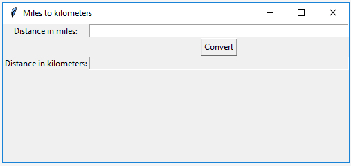
We are using a line input field to display the resulting distance in kilometers just to make things more symmetrical. Since we do not want the user to be able to enter anything into this text field, it has been disabled for input and we could just as easily have used another label widget. The Python code to create this tool with the help of tkinter is shown below and the explanation of the code follows.
from tkinter import Tk, Label, Entry, Button, DISABLED, StringVar

def convert():
    """Takes miles entered, converts them to km, and displays the result"""
    miles = float(entryMiles.get())
    kilometers.set(str(miles * 1.60934))

# create the GUI

rootWindow = Tk() # create main window
rootWindow.title("Miles to kilometers")
rootWindow.geometry('500x200+0+0')
rootWindow.grid_columnconfigure(1, weight = 1)

labelMiles = Label(rootWindow, text='Distance in miles:') # create label for miles field
labelMiles.grid(row=0, column=0)

labelKm = Label(rootWindow, text='Distance in kilometers:') # create label for km field
labelKm.grid(row=2, column=0)

entryMiles = Entry(rootWindow) # create entry field for miles
entryMiles.grid(row=0, column=1, sticky='w,e')

kilometers = StringVar() # create entry field for displaying km
entryKm = Entry(rootWindow, textvariable = kilometers, state=DISABLED)
entryKm.grid(row=2, column=1, sticky='w,e')

convertButton = Button(rootWindow, text='Convert', command = convert) # create button for running conversion
convertButton.grid(row=1, column=1)

# run the event processing loop

rootWindow.mainloop()
Let us ignore the first few lines of Python code for a moment and first look at lines 10 to 29. This is where the GUI of our little program is produced starting with the root window widget in lines 10 to 13. The widget is created by calling the function Tk() defined in tkinter and the created object is stored in variable rootWindow. We then use different methods of the widget to set its title, initial size, and some properties for its grid layout that we are going to use to arrange the child widgets within the content area of the root window.
Next, the label saying “Distance in miles:” is created. The tkinter widget class for labels is called Label and we provide rootWindow as a parameter to Label(…), so that the widget knows what its parent widget is. As mentioned, we will be using a grid layout, namely one with three rows and two columns. We place the created label in the cell in the first row and first column of its parent by calling the grid(…) method with row = 0 and column = 0. We then take the exact same steps to create the other label and place it in the third row of the first column.
In the next steps, the two text input fields are created as widget objects of the tkinter Entry class. An additional parameter sticky=’w,e’ is used for placing these widgets in the grid. This parameter says that the widgets should expand horizontally (west and east) to fill the entire cell. This is required to make the layout fill out the window horizontally and have the text field grow and shrink when the window is resized. Moreover, the Entry widget for displaying the distance in kilometers is set to DISABLED so that the user cannot enter text into it, and it is associated with a variable kilometers of tkinter class StringVar which is needed for us to be able to change the text displayed in the widget from code.
Finally, the button is created as a widget of tkinter class Button. What is new here is what happens with the ‘command’ parameter given to Button(…) in line 28. Here we are saying that if this button is clicked, the function convert() that we are defining at the top of our code should be executed to deal with this event. So this is an example of connecting an event to an event handler function. What happens in convert() is very simple: With the help of the get() method, we get the current text from the Entry widget for the distance in miles, multiply it with a constant to convert it to kilometers, and then use the set() method of the StringVar object in variable kilometers to change the text displayed in the Entry widget to the distance in kilometers associated with that variable.
In the last line of the code, we call the mainloop() method of our root window to start the infinite event processing loop. The program execution will only return from this call when the user closes the root window, in which case the program execution will be terminated.
The only part of the code we haven’t talked about is the first line where we simply import the widget classes and other auxiliary classes from tkinter that we need in our code.
Hopefully, it is clear that this is just a very prototypical implementation of a miles-to-kilometers conversion tool focusing on the GUI. We have neither implemented any sort of checking whether input values are valid nor any sort of error handling. It is therefore very easy to make the tool crash, e.g. by entering something that is not a number into the field for distance in miles. If you haven’t already done so, we suggest you create a Python script with the code from above and try out the tool yourself and see how the layout adapts if you resize the window. Feel free to experiment with making small changes to the code, like adapting the text shown by the labels or adding another button widget to the currently still empty second row of the first column; then make the button call another event handler function you write to, for instance, just print some message to the console.
Don’t worry if some of the details happening here don’t seem entirely clear at the moment. A real introduction to creating GUIs with Python will follow later in this lesson. Here we just wanted to give you a general idea of how the different concepts we discussed in Section 2.4 are realized in tkinter: You saw how different widgets are created, how they were arranged in a grid layout by placing them in different cells of the layout, how to connect an event (button clicked) with a self-defined event handler function (convert()), and how to execute the application by starting the event processing loop (rootWindow.mainloop()). Now let’s move on and talk about QT as an alternative to tkinter and see how this same example would look like when produced with the PyQt instead of tkinter.
2.5.2 QT
We already mentioned a few things about QT in this lesson. It is a widely used cross-platform library written in C++, modern and under very active development. In addition to the GUI functionality, the library provides support for internationalization, Unicode, database and network access, XML and JSON code processing, thread management, and more. That’s why it is also called an application framework, not just a GUI library. QT was originally developed by the company Trolltech and its initial release was in 1995. KDE, one of the early GUIs for the Linux operating system, was based on QT and that triggered a lot of discussion and changes to the license and organization QT was published under. These days, the company developing QT is called The QT Company, a successor of Trolltech, and QT is published in four different editions, including the Community edition that is available under different open source licenses GPL 3.0, LGPL 3.0, and LPGL 2.1 with a special QT exception. QT is very commonly used for both open source and commercial software, and if you have worked with QT in one programming language, it is typically relatively easy to learn to use it in a different language. QT5 was released in 2012 and the current version of QT at the time of this writing is 5.10.
2.5.2.1 PyQt vs. PySide
You may wonder why there exist two different Python wrappers for QT and how different they are? The short answer is that the reason lies mainly in license related issues and that PyQt and PySide are actually very similar, so similar that the code below for a QT based version of the miles-to-kilometers converter works with both PyQt and PySide. For PySide you only have to replace the import line at the beginning.
PyQt is significantly older than PySide and, partially due to that, has a larger community and is usually ahead when it comes to adopting new developments. It is mainly developed by Riverbank Computing Limited and distributed under GPL v3 and a commercial license. Releases follow a regular schedule and the software is generally considered very robust, mature, and well supported.
PySide is developed by Nokia and had its initial release in 2009, in a time when Nokia was the owner of QT. As can be read on the PySide web page, PySide has been developed and published in response to a lack of a QT wrapper for Python that has a suitable license for FOSS and proprietary software development. Without going too much into the details of the different license models involved, if you want to develop a commercial application, PyQt requires you to pay fees for a commercial license, while the LGPL license of PySide permits application in commercial projects.
From an educational perspective, it doesn’t really matter whether you use PySide or PyQt. As we already indicated, the programming interfaces have over the recent years converged to be very similar, at least for the basic GUI based applications we are going to develop in this course. However, we have some specific reasons to continue with PyQt that will be listed at the end of the next section. If you are interested to learn more about the differences between PyQt and PySide and when to pick which of the two options, the following blog post could serve as a starting point:
2.5.2.2 Installing PyQt5 from ArcGIS Pro
Since in contrast to tkinter, PyQt5 is not part of the Python standard library, we may need to install the PyQt5 package before we can use it from our code. We are currently using the Python installation that comes with ArcGIS Pro. Therefore, we will use the conda installation manager from within ArcGIS Pro to check whether PyQt5 is installed and if not, install it with all the packages it depends on. This will also automatically install the binary QT5 library that the PyQt5 package is a wrapper for.
Go ahead and open the package manager in Pro (Project -> Python) and check the Installed Packages list to see if "pyqt" is installed. If not, go to Add Packages and install "pyqt"; the process is identical to our installation of spyder back in Lesson 1.
You probably will now have version 5.9.2 or later of pyqt installed. Next, try to run the test code on the next page. If this code gives you an error of...
This application failed to start because it could not find or load the Qt platform plugin "windows".
...then you will need to come back to this page and set the QT_QPA_PLATFORM_PLUGIN_PATH environmental variable to the path of the plugin folder of PyQt5 (as explained in the blog post Developing Python GUI in ArcGIS Pro with PyQt). This can be done with the Windows tool for setting environmental variables by following the instructions below:
- Go to the Windows "Settings" and type “environmental” into the "Find a setting" search field and then pick “Edit the system environment variables”.
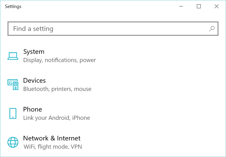 Figure 2.8 Windows "Settings" dialog
 - Click on “Environment variables…” at the bottom.
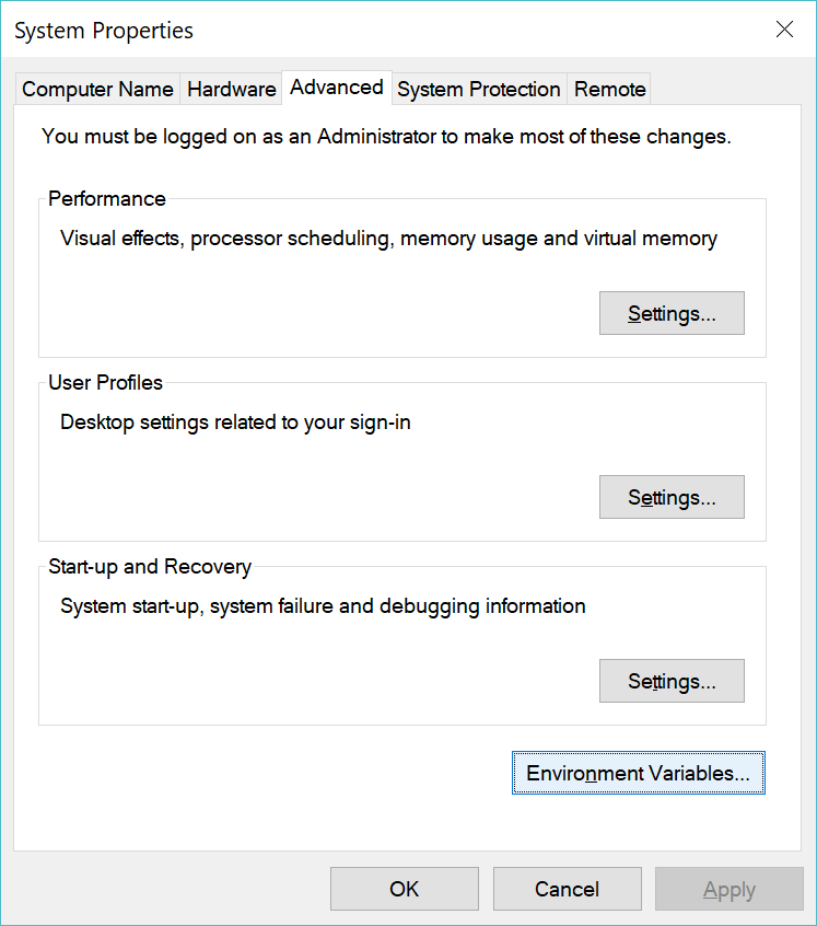 Figure 2.9 System Properties dialog with "Environment Variables..." button at the bottom right
 - Click on "New..." to add the environment variable at the bottom for "System variables".
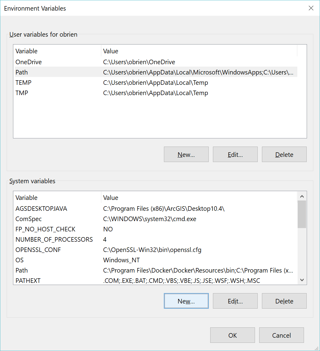 Figure 2.10 Variables dialog with "New..." button at the bottom
 - Fill out the dialog for adding a new variable. If the folder for your cloned ArcGIS Pro Python environment is something like "C:\Users\<username>\AppData\Local\ESRI\conda\envs\arcgispro-py3-clone", then use this to fill out the "Variable value" as shown in the figure below (see Section 1.5 explaining how opening Python Command Prompt will show the default folder). If you are using an older version of Pro and the default Python environment at "C:\Program Files\ArcGIS\Pro\bin\Python\envs\arcgispro-py3", then use this for the Variable value instead. Then press Ok and you are done.
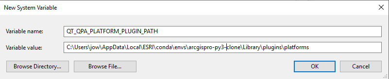 Figure 2.11 System Environment Variables dialog shown with variable name and variable value populated
2.5.2.3 Miles to kilometers with PyQT
Here is how the code for our miles-to-kilometers conversion tool looks when using PyQt5 instead of tkinter. You will see that there are some differences but a lot also looks very similar. We kept the names of the variables the same even though the widgets are named a little differently now. Since you now have PyQt5 installed, you can immediately run the code yourself and check out the resulting GUI. The result should look like the figure below.
Important note: When you run PyQt5 code in Spyder directly (here or in later sections), you may run into the situation that the program won't run anymore when you start it a second time and instead you get the error message "Kernel died, restarting" in the Spyder Python window. This can be resolved by going into the Spyder Preferences and under "Run" select the option "Remove all variables before execution" to make sure that everything from the previous run is completely cleaned up before the script code is executed again.
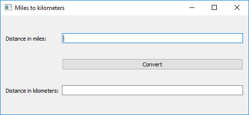
Source code:
from PyQt5.QtWidgets import QApplication, QWidget, QLabel, QGridLayout, QLineEdit, QPushButton

def convert():
    """Takes miles entered, converts them to km, and displays the result"""
    miles = float(entryMiles.text())
    entryKm.setText(str(miles * 1.60934))

app = QApplication([])

rootWindow = QWidget()
rootWindow.setWindowTitle("Miles to kilometers")
rootWindow.resize(500, 200)

gridLayout = QGridLayout(rootWindow)

labelMiles = QLabel('Distance in miles:')
gridLayout.addWidget(labelMiles, 0, 0)

labelKm = QLabel('Distance in kilometers:')
gridLayout.addWidget(labelKm, 2, 0)

entryMiles = QLineEdit()
gridLayout.addWidget(entryMiles, 0, 1)

entryKm = QLineEdit()
gridLayout.addWidget(entryKm, 2, 1)

convertButton = QPushButton('Convert')
gridLayout.addWidget(convertButton, 1, 1)

convertButton.clicked.connect(convert)

rootWindow.show()

app.exec_()
Let’s look at the main differences between this code and the tkinter based code from Section 2.5.1.
Obviously, we are now importing classes from the module PyQt5.QtWidgets and the widgets are named differently (all starting with ‘Q’).
While with tkinter, we only created one object for the application and root window together and then called its mainloop() method to start the execution of the event processing loop, the application and its main window are two different things in QT. In line 8, we create the application object and then at the very end we call its exec_() method to start the event processing loop. The window is created separately in line 10, and before we call exec_(), we invoke its show() method to make sure it is visible on the screen.
The creation of the widgets looks very similar in both versions. However, with tkinter, we didn’t have to create a grid layout explicitly; it was already available after the main window had been created. With PyQt5, we create the grid layout for the root window explicitly in line 14. To add widgets to the grid layout, we call the addWidget(…) method of the layout providing numbers for the row and column as paramters.
In the tkinter version, we had to set up a special variable to change the content of the entryKm line input field. This is not required with PyQt5. We can simply change the text displayed by the corresponding QLineEdit widget by calling its setText(…) method from the convert() function in line 6.
Finally, connecting the “clicked” event of the button with our convert() event handler function happens as a separate command in line 31 rather than via a parameter when creating the button object. By writing "convertButton.clicked.connect(convert)" we are saying, in QT terminology, that the “clicked” signal of convertButton should be connected to our convert() function.
It seems fair to say that from the perspective of the code, the differences between tkinter and PyQt5 are rather minor with, in some cases, one of them needing a bit more code, and in other cases, the other. However, this is partially due to this example being very simple and not involving more advanced and complex widgets and layouts.
When you tried out both versions of our little tool or just closely compared the two figures above with screenshots of the produced GUIs, you may also have noticed that, in addition to the differences in the code, there are some differences in the produced layout and behavior. We didn’t make use of all available options to make the two versions appear very similarly and it is certainly possible to do so, but our personal impression is that just based on the default look and behavior, the layout produced by PyQt5 is a bit more visually appealing. However, the main reason why we are going to continue with QT5/PyQt5 for the remainder of this lesson are the following:
- QT5 is a modern and widely used cross-platform and cross-language library; knowledge and skills acquired with QT can be applied in languages other than Python.
- QT5 is efficient and smooth because of the compiled core library written in C++.
- QT5 and PyQt5 provide a large collection of available widgets and can be expected to be under active development for the foreseeable future.
- There exists very good tool support for the combination of QT5 and PyQt5
- Finally and very importantly: In lesson 4 we will continue with the GUI development started in this lesson in the context of QGIS 3. QGIS and its interface for plugins have been developed for PyQt5.
As a final note, if you want to run the converter tool code with PySide, you have to replace the import line with the following line:
from PySide2.QtWidgets import QApplication, QWidget, QLabel, QGridLayout, QLineEdit, QPushButton
Of course, you will first have to install the PySide2 package in the ArcGIS Pro package manager to be able to run the code.
2.6 GUI development with QT5 and PyQt5
It is now time for a more systematic introduction to Python GUI development with QT5 and PyQt5. We will split this introduction into two parts, first showing you how to create GUI programmatically from Python code and then familiarizing you with the QT Designer tool for visually building GUIs and then translating them to Python code. In the walkthrough from Section 2.7, you will then work through a larger example of creating a GUI based application.
2.6.1 The manual approach
To familiarize ourselves with PyQT5 and get to know the most common QT5 widgets, let’s go through three smaller examples.
2.6.1.1 Example 1
Let’s start by just producing a simple window that has a title and displays some simple text via a label widget as shown in the image below.
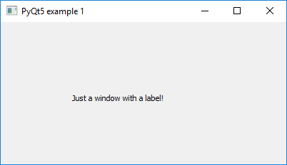
Thanks to PyQt5, the code for producing this window takes only a few lines:
import sys
from PyQt5.QtWidgets import QWidget, QApplication, QLabel

app = QApplication(sys.argv)

window = QWidget()
window.resize(400,200)
window.setWindowTitle("PyQt5 example 1")

label = QLabel("Just a window with a label!", window)
label.move(100,100)

window.show()

sys.exit(app.exec_())
Try out this example by typing or pasting the code into a new Python script and running it. You should get the same window as shown in the image above. Let’s briefly go through what is happening in the code:
- First of all, for each Python program that uses PyQT5, we need to create an object of the QApplication class that takes care of the needed initializations and manages things in the background. This happens in line 4 and we store the resulting QApplication object in variable app. At the very end of the program after setting up the different GUI elements, we use app.exec_() to call the exec_() method of the application object to run the application and process user input. The return value is used to exit the script by calling the sys.exit(…) function from the Python standard library. These are things that will look identical in pretty much any PyQT application.
- Most visible GUI elements (windows, button, text labels, input fields, etc.) in QT are derived in some way from the QWidget class and therefore called widgets. Widgets can be containers for other widgets, e.g. a window widget can contain a widget for a text label as in this example here. We are importing the different widgets we need here together with the QApplication class from the PyQt5.Widgets module in line 2. For our window, we directly use a QWidget object that we create in line 6 and store in variable window. In the following two lines, we invoke the resize(…) and setWindowTitle(…) methods to set the size of the window in terms of pixel width and height and to set the title shown at the top to “PyQt5 example 1”. After creating the other GUI elements, we call the show() method of the widget in line 13 to make the window appear on the screen.
- The content of the window is very simple in this case and consists of a single QLabel widget that we create in line 10 providing the text it should display as a parameter. We then use a fixed coordinate to display the label widget at pixel position 100,100 within the local reference frame of the containing QWidget. These coordinates are measured from the top left corner of the widget’s content area.
That’s all that’s needed! You will see that even if you resize the window, the label will always remain at the same fixed position.
If you have trouble running this script (e.g., you get a "Kernel died, restarting" error), try this version of the code (modified lines highlighted):
import sys
from PyQt5.QtWidgets import QWidget, QApplication, QLabel
from PyQt5.QtCore import Qt, QCoreApplication

app = QCoreApplication.instance()
if app is None:
    app = QApplication(sys.argv)

app.aboutToQuit.connect(app.deleteLater)

window = QWidget()
window.resize(400,200)
window.setWindowTitle("PyQt5 example 1")

label = QLabel("Just a window with a label!", window)
label.move(100,100)

window.show()

sys.exit(app.exec_())
This version of the code checks to see if there's already a QApplication object left existing in the current process -- only one of these objects is allowed. If an object exists, it's used; else, a new one is created. Line 9 then ensures that the application is deleted upon quitting.
As we already pointed out in Section 2.4.2, using absolute coordinates has a lot of disadvantages and rarely happens when building GUIs. So let’s adapt the example code to use relative layouts and alignment properties to keep the label always nicely centered in the middle of the window. Here is the code with the main changes highlighted:
import sys
from PyQt5.QtWidgets import QWidget, QApplication, QLabel, QGridLayout
from PyQt5.QtCore import Qt

app = QApplication(sys.argv)

window = QWidget()
window.resize(400,200)
window.setWindowTitle("PyQt5 example 1")

layout = QGridLayout(window)

label = QLabel("Just a window with a label (now perfectly centered!)")
label.setAlignment(Qt.AlignCenter)
layout.addWidget(label,0,0)

window.show()

sys.exit(app.exec_())
Try out this modified version and see whether you notice the change. Here is an explanation:
- For this simple example, different layouts would have worked, but we here use a QGridLayout for the window content that allows for arranging the child elements in a table–like way with the rows and columns being resized automatically to arrange everything in an optimal way given the available space. The grid layout object is created in line 11 and stored in variable layout. By providing window as the parameter, it is directly applied to manage the child elements of our window widget.
- The cells in the grid are accessed via their row and column indices starting from zero. In this example, we only have a single cell that will span the entire window. We add the label widget to this cell by calling the addWidget(…) method of the grid layout in variable layout and providing the coordinates 0,0 of the top left cell.
- Without any further changes, the label would now appear vertically centered in the window because that is the default policy for the cells in a grid layout, but horizontally adjusted to the left. To also make the label appear horizontally centered, we use its setAlignment(…) method with the constant Qt.AlignCenter that is defined in the PyQt5.QtCore module which we are also importing at the beginning.
If you tried out the modified example, you will have noticed that the label now always remains in the center independent of how you resize the window. That is the result of the grid layout manager working in the background to rearrange the child elements whenever the size is changed.
As a further extension of this example, let us make things a bit more interesting and bring in some interactions by adding a button that can be used to close the application as an alternative to using the close icon at the top. The widget needed to implement such a button is called QPushButton. We will add the button to cell 1,0 which is the cell in row 1 and column 0, so below the cell containing the label. That means that the grid layout will now consist of one column and two rows. Here is the modified code with the main changes highlighted:
import sys
from PyQt5.QtWidgets import QWidget, QApplication, QLabel, QGridLayout, QPushButton
from PyQt5.QtCore import Qt

app = QApplication(sys.argv)

window = QWidget()
window.resize(400,200)
window.setWindowTitle("PyQt5 example 1")

layout = QGridLayout(window)

label = QLabel("Just a window with a label (now perfectly centered!)")
label.setAlignment(Qt.AlignCenter)
layout.addWidget(label,0,0)

button = QPushButton("Close me")
button.setToolTip('This is a QPushButton widget. Clicking it will close the program!')
layout.addWidget(button,1,0)

button.clicked.connect(app.quit)

window.show()

sys.exit(app.exec_())
Please note how the push button widget is created in line 17 providing the text it will display as a parameter. It is then added to the layout in line 19. In addition, we use the setToolTip(…) method to specify the text that should be displayed if you hover over the button with the mouse. This method can be used for pretty much any widget to provide some help text for the user. The interesting part happens in line 21: Here we specify what should actually happen when the button is pressed by, in QT terminology, “connecting a signal (button.clicked) of the button to a slot (app.quit) of the application object”. So if the button is clicked causing a “clicked” event, the method quit(…) of the application object is called and the program is terminated as a result. Give this example a try and test out the tooltip and button functionality. The produced window should look like in the image below:
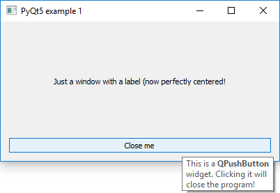
As you probably noticed, the button right now only takes up a fixed small amount of space in the vertical dimension, while most of the vertical space is taken by the cell containing the label which remains centered in this area. Horizontally, the button is expanded to always cover the entire available space. This is the result of the interplay between the layout policies of the containing grid layout and the button object itself. By default, the vertical policy of the button is set to always take up a fixed amount of space but the horizontal policy allows for expanding the button. Since the default of the grid layout is to expand the contained objects to cover the entire cell space, we get this very wide button.
In the last version of this first example, we are therefore going to change things so that the button is not horizontally expanded anymore by adding a QHBoxLayout to the bottom cell of the grid layout. This is supposed to illustrate how different widgets and layouts can be nested to realize more complex arrangements of GUI elements. In addition, we change the code to not close the application anymore when the button is clicked but instead call our own function that counts how often the button has been clicked and displays the result with the help of our label widget. A screenshot of this new version and the modified code with the main changes highlighted are shown below.
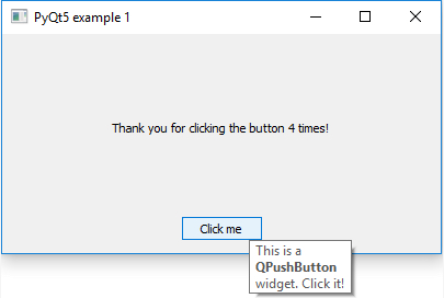
Source code:
import sys

from PyQt5.QtWidgets import QWidget, QApplication, QLabel, QGridLayout, QPushButton, QHBoxLayout
from PyQt5.QtCore import Qt

def buttonClickedHandler(c):
     global counter
     counter += 1
     label.setText('Thank you for clicking the button ' + str(counter) + ' times!')

app = QApplication(sys.argv)

window = QWidget()
window.resize(400,200)
window.setWindowTitle("PyQt5 example 1")

layout = QGridLayout(window)

label = QLabel("Just a window with a label (now perfectly centered!)")
label.setAlignment(Qt.AlignCenter)
layout.addWidget(label,0,0)

button = QPushButton("Click me")
button.setToolTip('This is a QPushButton widget. Click it!')

horLayout = QHBoxLayout()
horLayout.addStretch(1)
horLayout.addWidget(button)
horLayout.addStretch(1)
layout.addLayout(horLayout,1,0)

button.clicked.connect(buttonClickedHandler)

counter = 0

window.show()

sys.exit(app.exec_())
In addition to the highlighted changes, there are a few very minor changes to the text displayed on the button and its tooltip. Let us first look at the changes made to implement the counting when the button is pressed. Instead of directly connecting the button.clicked signal to the slot of another QT element, we are connecting it to our own function buttonClickedHandler(…) in line 32. In addition, we create a global variable counter for counting how often the button has been clicked. When it is clicked, the buttonClickedHandler(…) function defined in lines 6 to 9 will be called, which first increases the value of the global counter variable by one and then uses the setText(…) method of our label object to display a message which includes the number of button presses taken from variable counter. Very simple!
Now regarding the changes to the layout to avoid that the button is expanded horizontally: In principle, the same thing could have been achieved by modifying the horizontal layout policy of the button. Instead, we add a new layout manager object of type QHBoxLayout to the bottom cell of the grid layout that allows for arranging multiple widgets in horizontal order. This kind of layout would also be a good choice if, for instance, we wanted to have several buttons at the bottom instead of just one, all next to each other. In line 26, we create the layout object and store it in variable horLayout. Later in line 30, we add the layout to the bottom cell of the grid layout instead of adding the button directly. This is done using the addLayout(…) method rather than addWidget(…).
In between these two steps, we add the button to the new horizontal layout in horLayout in line 28. In addition, we add horizontal stretch objects to the layout before and after the button in lines 27 and 29. We can think of these objects as springs that try to take up as much space as possible without compressing other objects more than these allow. The number given to the addStretch(…) method is a weight factor that determines how multiple stretch objects split up available space between them. Since we use 1 for both calls of addStretch(…), the button will appear horizontally centered and just take up as much space as needed to display its text. If you want to have the button either centered to the left or to the right, you would have to comment out line 27 or line 29, respectively. What do you think would happen if you change the weight number in line 27 to 2, while keeping the one in line 29 as 1? Give it a try!
2.6.1.2 Example 2
We are now moving on to example 2, a completely new example that focuses on the menu bar and status bar widgets as well as on defining user actions that can be associated with different input widgets and some other useful features of QT5 that are commonly used in GUI-based programs. Often GUI-based programs provide many ways in which the user can trigger a particular action, e.g. the action for saving the currently opened file can typically be performed by choosing the corresponding entry from the menu bar at the top, by a keyboard shortcut like CTRL+S for instance, and potentially also by a tool button in a toolbar and by some entry in a so-called context menu that shows up when you click the right mouse button. PyQT5 provides the QAction class for defining actions and these actions can then be associated with or added to different GUI elements that are supposed to trigger the action. For instance, in the following example we will create an action for exiting the program with the following four lines of code:
exitAction = QAction(app.style().standardIcon(QStyle.SP_DialogCancelButton’), '&Exit', mainWindow)

exitAction.setShortcut('Ctrl+Q')

exitAction.setStatusTip('Exit application')

exitAction.triggered.connect(app.quit)
The QAction object for our exit action is created in the first line and then stored in variable exitAction. The first two parameters given to QAction(…) are an icon that will be associated with that action and the name. For the icon we use the SP_DialogCancelButton icon from the set of icons that comes with QT5. Of course, it is possible to use your own set of icons but we want to keep things simple here. The & symbol in the name of the action (&Exit) signals that it should be possible to use ALT+E as a keyboard shortcut to trigger the action when using the application’s menu bar. The last parameter is the parent object which needs be another QT object, the one for the application’s main window in this case (more on this in a moment).
In the following two lines we define the keyboard shortcut (Ctrl+Q) that can be used at any moment to trigger the action and a message that should be shown in the status bar (the bar at the bottom of the application’s main window that is typically used for showing status messages) when hovering over a GUI element that would trigger this action. Finally, in the last line we connect the event that our exit action is triggered (by whatever GUI element) to the quit slot of our application. So this is the part where we specify what the action should actually do and as we have seen before, we can either connect the signal directly to a slot of another GUI element or to a function that we defined ourselves.
We already briefly mentioned the “main window” of the application. In example 1 above, we used the QWidget object for the main window and container of the other GUI elements. In example 2, we will use the QMainWindow widget instead which represents a typical application window with potentially a menu bar and tool bar at the top, a large central area in the middle to display the main content of the app, and potentially a small status bar at the bottom. The image below shows how the main window we are going to create in example 2 will look.
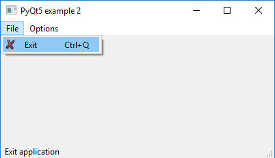
Once a QMainWindow object has been created and stored in variable mainWindow, its menu bar (an object of type QMenuBar that is created automatically) can be accessed via the menuBar() method, so with the expression mainWindow.menuBar(). A menu bar consists of one or more menus (= objects of the QMenu class) which in turn consist of several menu entries. The entries can be actions or submenus which again are QMenu objects. To add a new menu to a menu bar, you call its addMenu(…) method and provide the name of the menu, for instance ‘&File’. The method returns the newly created QMenu object as a result, so that you can use it to add menu entries to it. To add an action to a menu, you invoke a method called addAction(…) of the menu object, providing the action as a parameter. With that explanation, it should be relatively easy to follow the code below. We have highlighted the important parts related to creating the main window, setting up the menu bar, and adding the exit action to it.
import sys

from PyQt5.QtWidgets import QApplication, QMainWindow, QAction, QStyle

app = QApplication(sys.argv)

mainWindow = QMainWindow()
mainWindow.resize(400,200)
mainWindow.setWindowTitle("PyQt5 example 2")

fileMenu = mainWindow.menuBar().addMenu('&File')
optionsMenu = mainWindow.menuBar().addMenu('&Options')

exitAction = QAction(app.style().standardIcon(QStyle.SP_DialogCancelButton), '&Exit', mainWindow)
exitAction.setShortcut('Ctrl+Q')
exitAction.setStatusTip('Exit application')
exitAction.triggered.connect(app.quit)

fileMenu.addAction(exitAction)

mainWindow.statusBar().showMessage('Waiting for your commands...')

mainWindow.show()

sys.exit(app.exec_())
The QMainWindow is created very similarly to the QWidget we used in example 1, meaning we can set the title and initial size of the widget (lines 8 and 9). The two menus ‘File’ and ‘Options’ are added to the menu bar of our main window in lines 11 and 12, and the QMenu objects returned are stored in variables fileMenu and optionsMenu, respectively. In line 19, we add the exit action we created with the code already discussed earlier (lines 14 to 17) to the ‘File’ menu. The icon and name we provided when creating the action will be used for the entry in the menu bar and selecting the entry will trigger the action and result in the quit() method of application being called.
Please note that in line 21, we also added a command to show a message in the status bar at the bottom of the main window when the application is started. The status bar object is accessed via the statusBar() method of the QMainWindow, and then we directly call its showMessage(…) method specifying the text that should be displayed. We suggest that you run the program a few times, trying out the different ways to exit it via the menu entry (either by clicking the entry in the ‘File’ menu or using ALT+F followed by ALT+E) and the action's keyboard shortcut CTRL+Q that we defined.
So far, our 'File' menu only has a single entry and the 'Options' menu is still completely empty. In the following, we are going to extend this example by adding ‘Open’ and ‘Save’ actions to the ‘File’ menu making it appear somewhat similar to what you often see in programs. We also add entries to the 'Options' menu, namely one with a checkbox next to it that we use for controlling whether the label displayed in our main window is shown or hidden, and one that is a QMenu object for a submenu with two additional entries. The two images below illustrate how our menu bar will look after these changes.
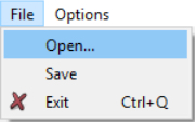
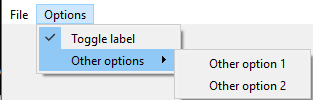
In addition to the changes to the menu bar, we will use the QFileDialog widget to display a dialog for selecting the file that should be opened and we use a QMessageBox widget to display a quick message to the user that the user has to confirm. Here is the code for the new version with main changes highlighted. Further explanation will follow below:
import sys

from PyQt5.QtWidgets import QApplication, QMainWindow, QAction, QStyle, QFileDialog, QMessageBox, QWidget, QGridLayout, QLabel, QMenu
from PyQt5.QtCore import Qt

def openFile():
     fileName, _ = QFileDialog.getOpenFileName(mainWindow, "Open file", "", "All files (*.*)")
     if fileName:
         mainWindow.statusBar().showMessage('User has picked file ' + fileName)
     else:
         mainWindow.statusBar().showMessage('User canceled the file dialog.')

def saveFile():
     QMessageBox.information(mainWindow, 'Important information', 'Save file has not been implemented yet, sorry!', QMessageBox.Ok)

def toggleLabel(state):
     if state:
         label.show()
     else:
         label.hide()

app = QApplication(sys.argv)

mainWindow = QMainWindow()
mainWindow.resize(400,200)
mainWindow.setWindowTitle("PyQt5 example 2")
mainWindow.setCentralWidget(QWidget())

layout = QGridLayout(mainWindow.centralWidget())

label = QLabel("Some text ...")
label.setAlignment(Qt.AlignCenter)
layout.addWidget(label,0,0)

fileMenu = mainWindow.menuBar().addMenu('&File')
optionsMenu = mainWindow.menuBar().addMenu('&Options')

openAction = QAction('&Open...', mainWindow)
openAction.triggered.connect(openFile)
fileMenu.addAction(openAction)

saveAction = QAction('&Save', mainWindow)
saveAction.triggered.connect(saveFile)
fileMenu.addAction(saveAction)

exitAction = QAction(app.style().standardIcon(QStyle.SP_DialogCancelButton), '&Exit', mainWindow)
exitAction.setShortcut('Ctrl+Q')
exitAction.setStatusTip('Exit application')
exitAction.triggered.connect(app.quit)
fileMenu.addAction(exitAction)

toggleLabelAction = QAction('&Toggle label', mainWindow, checkable=True)
toggleLabelAction.setChecked(True)
toggleLabelAction.triggered.connect(toggleLabel)
optionsMenu.addAction(toggleLabelAction)

otherOptionsSubmenu = QMenu('&Other options', mainWindow)
otherOption1Action = QAction('Other option &1', mainWindow, checkable=True)
otherOption2Action = QAction('Other option &2', mainWindow, checkable=True)

otherOptionsSubmenu.addAction(otherOption1Action)
otherOptionsSubmenu.addAction(otherOption2Action)
optionsMenu.addMenu(otherOptionsSubmenu)

mainWindow.statusBar().showMessage('Waiting for your commands...')

mainWindow.show()

sys.exit(app.exec_())
In addition to importing some more widgets and other PyQT classes that we need, we define three functions at the beginning, openFile(), saveFile(), and toggleLabel(…). These will serve as the event handler functions for some of the new actions/menu entries that we are adding, and we will discuss them in more detail later.
The next thing to note is that in lines 31 to 33 we are reintroducing our label object from the first example in the center of the main window. Since our window is based on QMainWindow, we first have to create a QWidget to fill the central area of the main window via its setCentralWidget(…) method (line 27), and then we add the needed layouts and QLabel object itself to this central widget exactly as in example 1 (lines 29 to 33).
In lines 38 and 42, we create new QAction objects for the two actions we want to add to the ‘File’ menu in variable fileMenu. To keep the code from getting too long, we don’t set up icons, keyboard shortcuts, and status bar tips for these like we did for the exit action, but these could be easily added. They are set up to call the openFile() and saveFile() functions we defined when they are triggered (lines 39 and 43), and both actions are added to fileMenu via the addAction(…) method in lines 40 and 44.
In lines 52 to 55, the action with the checkbox to toggle the label on and off is created and added to the ‘Options’ menu. The main difference to the other actions is that we use the additional keyword argument checkable=True when creating the action object in line 52, and then set the initial state to being checked in the following line. The "triggered" signal of the action is connected to the toggleLabel(…) function. Note how this function, in contrast to other event handler function we created before, has a parameter state that when called will be given the state of the action, meaning whether it is checked or unchecked, as a boolean. The code in the body of the function in lines 17 to 20 then simply checks whether this state is True for "checked" and if so, makes sure that the label is visible by calling its show() method. If state is False for "unchecked", it will call hide() instead and the label will become invisible.
In lines 57 to 63, we create a submenu for the ‘Options’ menu with two more checkable actions that we simply call ‘Other option 1’ and ‘Other option 2’. This is just for illustrating how to create a submenu in a menu bar, so we don’t bother with linking these actions to some actual functionality as we might in a real-world situation. The important part starts with line 57 where we create a QMenu object called ‘Other options’ that we then add the actions to in line 61 and 62. In line 63, we then add this new menu to our ‘Options’ menu in variable optionsMenu. Since we are not adding an action but a submenu here, we have to use the addMenu(…) method for this.
Now it is time to have a closer look at the openFile() and saveFile() functions that describe what should happen if the open or save actions are triggered. We are keeping things very simple in the saveFile() function, so let us start with that one: Since we are just creating a GUI framework here without real functionality, we only display a warning message to the user that no save file functionality has been implemented yet. We do this with the help of the QMessageBox widget that has the purpose of making, creating, and showing such message boxes as easily as possible. QMessageBox has several methods that can be invoked to display different kinds of messages such as simple information text or questions that require some user input. To just display some text and have an OK button that the user needs to click for confirmation, we use the information(…) method (line 14). We have to provide a parent QT object (mainWindow), a title, the information text, and the kind of buttons we want in the message box (QMessageBox.Ok) as parameters.
Finally, let’s look at the openFile() function in lines 6 to 11: here we illustrate what would typically happen when the action to open a file is triggered. Among other things, you typically want to provide a file browser dialog that allows the user to pick the file that should be opened. Such a dialog is much more complicated than a simple message box, so we cannot use QMessageBox for this, but fortunately QT provides the QFileDialog widget for such purposes. Like QMessageBox, QFileDialog has multiple methods that one can call depending on whether one needs a dialog for opening an existing file, selecting a folder, or saving a file under a name chosen by the user. We here use QFileDialog.getOpenFileName (…) and provide a parent object (mainWindow), a title for the dialog, and a string that specifies what files can be selected based on their file extension as parameters. For the last parameter, we use "*.*" meaning that the user can pick any file.
getOpenFileName (…) has a return value that indicates whether the user left the dialog via the Ok button or whether the user canceled the dialog. In the first case, the return value will be the name of the file selected, and in the second case it will be None. We capture this return value in variable fileName and then use an if-statement to distinguish both cases: In the first case, we use showMessage(…) of our status bar to display a message saying which file was selected. If the condition is False (so if fileName is None), we use the same message to inform that the dialog was canceled.
This second version of example 2 has already gotten quite long and the same applies for our explanation. You should take a moment to run the actual application and test out the different actions we implemented, the message box display, the open file dialog, toggling the label on and off via the entry under the ‘Options’ menu, and so on.
2.6.1.3 Example 3
We are now leaving the world of menu bars behind and moving on to a third and final example of manually creating PyQT5 based programs which has the purpose of showing you the most common widgets used for getting input from the user as well as the following things:
- how to build own dialog boxes from these widgets, similar to the open file dialog for example,
- how to arrange widgets in more complex ways,
- and how to use the created dialog boxes from the main code.
We will keep the actual functionality we have to implement in this example to a minimum and mainly connect signals sent by the different widgets to slots of other widgets. As a result, the dialog box will operate in a somewhat weird way and we, hence, call this example “The world’s weirdest dialog box”. It still serves the purpose of illustrating the different event types and how to react to them.
To understand the example, it is important to know that dialog boxes can be invoked in two different ways, modally and modelessly (also referred to as non-modal). Modal means that when the method for displaying the dialog to the user is called, it will only return from the call once the user closes the dialog (e.g. by pressing an Ok or Cancel button). That means the user cannot interact with any other parts of the program's GUI, only the dialog box. When a dialog is invoked in the modeless approach, the method for displaying the dialog will return immediately and the dialog will essentially be displayed in addition to the other windows of the program that still can be interacted with.
The QDialog widget that we will use to build our own dialog box in this example, therefore, has two methods: exec_() for displaying the dialog modally, and show() for displaying it in the modeless way. In contrast to show(), exec_() has a return value that indicates whether the dialog was canceled or has been closed normally, e.g. by pressing an Ok button. You may wonder how our program would be informed about the fact that the dialog has been closed, and in which way, in the modeless option using show(). This happens via the signals accepted and rejected that the dialog will produce in this case and that we can connect to in the usual way. You will see an example of that later on but we first start with a modal version of our dialog box.
The final version of example 3 will be even longer than that of example 2. We, therefore, added some comments to structure the code into different parts, e.g. for setting up the application and GUI, for defining the functions that realize the main functionality, for wiring things up by connecting signals to slots or functions, and so on. In case you run into any issues while going through the following steps to produce the final code for the example, the final script file can be downloaded here. In the first skeleton of the code shown below, some of the sections introduced by the comments are still empty but we will fill them while we move along. This first version only illustrates how to create an empty QDialog object for our dialog box and show it (modally) when a button located on the main window is clicked. The most important parts of the code are again highlighted.
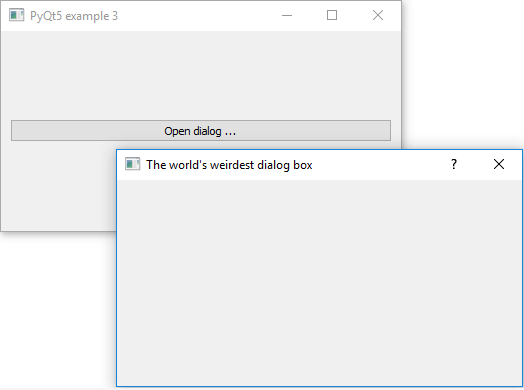
# imports

import sys
from PyQt5.QtWidgets import QApplication, QMainWindow, QPushButton, QGridLayout, QWidget, QDialog

# set up app and GUI

app = QApplication(sys.argv)

mainWindow = QMainWindow()
mainWindow.resize(400,200)
mainWindow.setWindowTitle("PyQt5 example 3")
mainWindow.setCentralWidget(QWidget())

layout = QGridLayout(mainWindow.centralWidget())

button = QPushButton("Open dialog ...")
layout.addWidget(button,0,0)

dialogBox = QDialog()
dialogBox.setWindowTitle("The world's weirdest dialog box")

# functions for interactions

# functions for modal version

# functions for modeless version

# connect signals and other initializations

button.clicked.connect(dialogBox.exec_) # invoke dialog modal version

# run the program

mainWindow.show()

sys.exit(app.exec_())
The QDialog widget is created in line 21 and it is stored in variable dialogBox. We can now add content (meaning other widgets) to it in a similar way as we did with QWidget objects in previous examples using the addWidget(…) and addLayout(…) methods. In lines 17 and 18, we create a simple push button and add it to our main window. In line 31, we connect the "clicked" signal of this button with the exec_() method of our (still empty) dialog box. As a result, when the button is pressed, exec_() will be called and the dialog box will be displayed on top of the main window in a modal way blocking the rest of the GUI. Run the application now and see whether the dialog shows up as expected when the button is clicked.
We are now going to add the widgets to our dialog box in variable dialogBox. The result should look as in the image below:
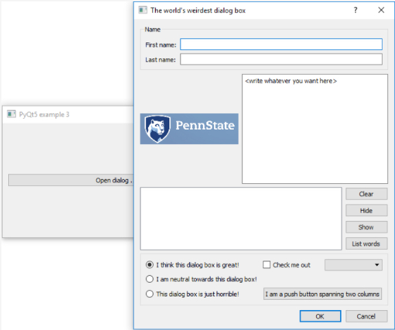
Please follow the steps below to create this new version of example 3:
Step 1. Replace all the lines with import statements under the comment “# imports” and before the comment “# set up app and GUI” with the following lines.
import sys, random

from PyQt5.QtWidgets import QApplication, QMainWindow, QPushButton, QGridLayout, QWidget, QDialog, \
   QVBoxLayout, QGroupBox, QLabel, QLineEdit, QTextEdit, QHBoxLayout, QListView, QRadioButton, \
   QCheckBox, QComboBox, QDialogButtonBox
from PyQt5.QtCore import Qt, QVariant
from PyQt5.QtGui import QPixmap, QStandardItemModel, QStandardItem
As you can see, we need to import quite a few more widget classes. In addition, using some of these will require additional auxiliary classes from the PyQt5.QtCore and PyQt5.QtGui modules.
Step 2. Keep the code that is currently under the comment “# set up app and GUI” as this will not change. But then add the following code directly after it, still before the “# functions for interactions” comment.
mainVerticalLayout = QVBoxLayout(dialogBox)

nameGroupBox = QGroupBox("Name") # row 1 of vertical layout
mainVerticalLayout.addWidget(nameGroupBox)
nameGridLayout = QGridLayout(nameGroupBox)
firstNameLabel = QLabel("First name:")
nameGridLayout.addWidget(firstNameLabel, 0, 0)
lastNameLabel = QLabel("Last name:")
nameGridLayout.addWidget(lastNameLabel, 1, 0)
firstNameLineEdit = QLineEdit()
nameGridLayout.addWidget(firstNameLineEdit, 0, 1)
lastNameLineEdit = QLineEdit()
nameGridLayout.addWidget(lastNameLineEdit, 1, 1)

imageHorizontalLayout = QHBoxLayout() # row 2
mainVerticalLayout.addLayout(imageHorizontalLayout)
imageLabel = QLabel()
imageLabel.setPixmap(QPixmap("psu.PNG").scaledToWidth(172))
imageHorizontalLayout.addWidget(imageLabel)
textEdit = QTextEdit()
textEdit.setText("<write whatever you want here>")
imageHorizontalLayout.addWidget(textEdit)

listGridLayout = QGridLayout() # row 3
mainVerticalLayout.addLayout(listGridLayout)
listView = QListView()
listGridLayout.addWidget(listView, 0, 0, 4, 1)
clearPushButton = QPushButton("Clear")
listGridLayout.addWidget(clearPushButton, 0, 1)
hidePushButton = QPushButton("Hide")
listGridLayout.addWidget(hidePushButton, 1, 1)
showPushButton = QPushButton("Show")
listGridLayout.addWidget(showPushButton, 2, 1)
listWordsPushButton = QPushButton("List words")
listGridLayout.addWidget(listWordsPushButton, 3, 1)

widgetGroupBox = QGroupBox() # row 4
mainVerticalLayout.addWidget(widgetGroupBox)
widgetGridLayout = QGridLayout(widgetGroupBox)
greatRadioButton = QRadioButton("I think this dialog box is great!")
greatRadioButton.setChecked(True)
widgetGridLayout.addWidget(greatRadioButton, 0, 0)
neutralRadioButton = QRadioButton("I am neutral towards this dialog box!")
widgetGridLayout.addWidget(neutralRadioButton, 1, 0)
horribleRadioButton = QRadioButton("This dialog box is just horrible!")
widgetGridLayout.addWidget(horribleRadioButton, 2, 0)
checkBox = QCheckBox("Check me out")
widgetGridLayout.addWidget(checkBox, 0, 1)
comboBox = QComboBox()
widgetGridLayout.addWidget(comboBox, 0, 2)
widgetPushButton = QPushButton("I am a push button spanning two columns")
widgetGridLayout.addWidget(widgetPushButton, 2, 1, 1, 2)

buttonBox = QDialogButtonBox() # row 5
buttonBox.setStandardButtons(QDialogButtonBox.Cancel | QDialogButtonBox.Ok)
mainVerticalLayout.addWidget(buttonBox)
This is the code for creating all the different widgets in our dialog box. You should be getting used to reading this kind of code, so we will just explain the most important points here:
- The overall organization of the dialog box is illustrated in the previous figure. The widgets are organized into five rows. This happens with a QVBoxLayout that arranges items vertically, each item below the previous one. The layout is created in line 1 and by using dialogBox as the parameter of QVBoxLayout(…), we are directly adding it to our dialog box. Each of the five following blocks of code create one of the rows in this vertical layout.
- The first block from line 3 to 13 is formed by a single QGroupBox item which in turn contains two QLabel and two QEditLine widgets. QEditLine widgets are used for allowing the user to enter a single line of text. The labels are just for describing what should be entered into the respective line edit widget. To make everything look tidy, we use a QGridLayout as in Example 1 or the miles-to-kilometers converter to arrange these items into two columns with the first one containing the labels and the second one containing the line edit widgets.
- The second row created in lines 15 to 22 is formed by two widgets, a QLabel that we will use to display an image of the PSU logo and a QTextEdit widget that allows for entering multi-line text. The label doesn’t have any text assigned. Instead, we use the method setPixmap(…) to assign it an image that will be displayed instead of text. You will need to download the Penn State logo here and place it in the same folder as the script to be able to run the program. To have these elements placed neatly next to each other, we use a QHBoxLayout as in Example 1 for this row and add the two widgets to it.
- Row 3 (lines 24 to 35) contains a QListView widget on the left and four QPushButtons arranged vertically on the right. The list view is intended for displaying a list of items, one per row, and potentially allowing the user to select one or multiple of these rows/items. We use another grid layout to arrange the items in this row. The grid has two columns and three rows (because of the four buttons) and what is new here is that we are setting up the list view widget to span all four rows. This happens in line 27 by providing two additional parameters to addWidget(…): 4 for the number of rows the widget should span and 1 for the number of columns.
- For row 4 in lines 37 to 52, we again use a group box and a grid layout (3 rows x 4 columns) to arrange the widgets inside the group box, and we add a diverse collection of different widgets to it: The first column is filled by three QRadioButtons. Radio buttons allow for picking one of several choices and it is used here in our dialog box to state your opinion on this dialog box ranging from great over neutral to horrible. The radio buttons inside the same group box are automatically linked so that when you select one, all others will be deselected. In addition, we also add a QCheckBox that can be checked and unchecked and a QComboBox for selecting one item from multiple choices. Finally we have another QPushButton, this time one that spans columns 2 and 3 (see line 52).
- The last row (lines 54 to 56) contains an “Ok” and a “Cancel” button. These are standard elements for a dialog box, so QT provides some easy way to set these up in the form of the QDialogButtonBox widget. We just have to tell the widget which buttons we want via the setStandardButtons(…) method in line 55.
At this point, you can run the script and it should produce the GUI as shown in the previous figure. You can already type things into the different edit fields and use the checkbox and radio buttons. The other elements still need to be connected to some functionality to serve a purpose, which is what we will do next.
Step 3. The next things we are going to add are two functions to put some content into the QListView widget in the third row and the QComboBox widget in the fourth row. Since we want to illustrate how different GUI elements can be connected to play together, we will use the list view to display a list of the words from the text that has been entered into the QTextEdit widget in the second row (variable textEdit). The combo box we will simply fill with a set of randomly generated numbers between 1 and 9. Then we will wire up these widgets as well as the push buttons from the third row and the QDialogButtonBox buttons from the fifth row.
The following code needs to be placed directly under the comment “# functions for interactions”, before the comment “# functions for modal version”.
def populateListView():
     words = textEdit.toPlainText().split()
     m = QStandardItemModel()
     for w in words:
         item = QStandardItem(w)
         item.setFlags(Qt.ItemIsUserCheckable | Qt.ItemIsEnabled)
         item.setData(QVariant(Qt.Checked), Qt.CheckStateRole)
         m.appendRow(item)
     listView.setModel(m)

def populateComboBoxWithRandomNumbers():
     comboBox.clear()
     for i in range(5):
         comboBox.addItem(str(random.randrange(10)))
The function populateListView() calls the method toPlainText() of the QTextEdit widget. The QTextEdit widget can contain rich text with styling but this method only gives us the plain text without styling markups as a string. We then use the string method split() to split this string into a list of strings at each space or other whitespace symbol. The resulting list of words is stored in variable words. The QListView is one of the widgets that needs a model behind it meaning some object that stores the actual list data to be displayed. Since we just need a list of simple string objects here, we use the QStandardItemModel class available for such cases and fill it with QStandardItem objects we create, one for each word in our words list (lines 3 to 8). The model created in this way is then given to the setModel() method of the list view, which will then display these items. In lines 6 and 7 we are setting up the list items to have a check box that is originally checked but can be unchecked by the user to only select a subset of the items.
Populating the combo box with items the user can pick from is much simpler because we can directly add string items to it with the addItem(…) method (line 14). In the populateComboBoxWithRandomNumbers() function, we first clear the current content, then use a for-loop that creates the random numbers and adds them as string items to the combo box.
In addition, you now need to place the following lines of code directly under the comment “# connect signals and other initializations”, before the line that is already there for opening the dialog when the button on the main window is clicked:
radioButtons = [ greatRadioButton, neutralRadioButton, horribleRadioButton ]

populateComboBoxWithRandomNumbers()

buttonBox.accepted.connect(dialogBox.accept)
buttonBox.rejected.connect(dialogBox.reject)
clearPushButton.clicked.connect(textEdit.clear)
hidePushButton.clicked.connect(textEdit.hide)
showPushButton.clicked.connect(textEdit.show)
listWordsPushButton.clicked.connect(populateListView)
The first line will only play a role later on, so we ignore it for the moment. In line 3, we call the populateComboBoxWithRandomNumbers() function to initialize the combo box so that it contains a list of numbers immediately when the dialog box is opened for the first time. Next we wire up the “Ok” and “Cancel” buttons for exiting the dialog (lines 5 and 6). This is not done via the "clicked" signals of the button themselves but via the "accepted" and "rejected" signals of the button box that contains them. We connect these signals to the accept() and reject() methods of our dialog box, and these will take care of producing the corresponding return values or trigger the corresponding signals depending on whether we called the dialog box modally or modeless.
Finally, we connect the four push buttons from the third row (lines 7 to 10). The first three are used to invoke different methods of the text edit widget above them: The first clears the text area, the second hides the widget, and the third shows it again. The fourth button is set up to invoke our populateListView() function, so this is the button that needs to be clicked for a list of words to show up in the list view widget. Go ahead and run the script now. Enter a few lines of text into the text edit field and then click the “List words” button and observe the list of words that can now be selected via the little checkboxes. Then try out the other buttons and the combo box.
Step 4. At this point, we still have a few widgets in our dialog box that do not do anything. Let’s make things really weird by adding the following commands to the “# connect signals and other initializations” section directly following the lines you just added and still before the line for opening the dialog when the button on the main window is clicked.
widgetPushButton.pressed.connect(populateComboBoxWithRandomNumbers)
firstNameLineEdit.textChanged.connect(checkBox.toggle)
lastNameLineEdit.editingFinished.connect(comboBox.showPopup)
Take a brief moment to read these commands and try to understand the functionality they are adding. Do you understand what is happening here? The first line is for finally giving some functionality to the large push button labeled “I am a push button spanning two row”. We connect this button to our function for populating the combo box with random numbers. So every time you click the button, the combo box will show a different selection of random numbers to pick from. Please note that we are not connecting the "clicked" signal here as we did with the other push buttons. Instead, we connect the "pressed" signal. What is the difference? Well, the "clicked" signal will only be sent out when the mouse button is released, while "pressed" is immediately sent when you press down the mouse button. When you run the dialog again, check out whether you notice the difference.
In the second and third line, we do something that you would usually never do in a dialog box: We connect the "textChanged" signal of the line edit widget for entering your first name at the top to the "toggle" slot of our checkbox widget in the fourth row. This signal is emitted whenever the text in the field is changed, e.g. every time you press a key while editing this input field. So if you type in your first name, you will see the checkbox constantly toggle between its checked and unchecked states. We then connect the "editingFinished" signal of the line edit widget for the last name to the "showPopup" slot of our combo box for opening the drop down list with the different choices. The difference between "textChanged" and "editingFinished" is that "editingFinished" will only be emitted when you press TAB or the widget loses focus in another way, for instance when you click on a different widget. So if you enter your last name and press TAB, you will see the drop down list of the combo box appearing. Give this and the other weird things we just implemented a try by running the script!
Step 5. It’s probably best if we stop wiring up our dialog box at this point, but feel free to keep experimenting with the different signals and connecting them to different slots later on after we have completed this example. We now want to focus on what typically happens if the dialog box is closed. Right now, nothing will happen because we have been connecting the push button on our main window directly to the exec_() method, so there is no own code yet that would be executed when returning from this method. Typically, you will have your own function that calls exec_() and that contains some additional code depending on whether the user closed the dialog via the “Ok” or “Cancel” button and the state or content of the different widgets. For this purpose, please first add the following function at the end of the “# functions for interactions” section, directly before “# functions for modal version”:
def printResults():
     for rb in radioButtons:
         if rb.isChecked():
             print("Selected opinion: " + rb.text())
     print("Combo box has current value " + comboBox.currentText())
     print("Checkbox is " + ("checked" if checkBox.isChecked() else "unchecked"))
Then under "#functions for modal version" insert the following code:
def openDialogModal():
     result = dialogBox.exec_()
     if result == QDialog.Accepted:
         printResults()
     else:
         print("Exited dialog via cancel button or closing window")
Finally, change the line in which we set up the main window button to open the dialog from
button.clicked.connect(dialogBox.exec_()) # invoke dialog modal version
to
button.clicked.connect(openDialogModal) # invoke dialog modal version
It should be clear that this last change means that instead of opening the dialog box directly, we are now calling our own function openDialogModal() when the button on the main window is clicked. Looking at the code of that function, the first thing that will happen then is that we call dialogBox.exec_() to open the dialog box, but here we also capture its return value in variable result. When the dialog box is closed, this return value will tell us whether the user accepted the dialog (the user clicked ok) or whether the user rejected the dialog (the user clicked cancel or closed the dialog in another way). The return value is a number but instead of bothering with how accepted and rejected are encoded, we compare result to the corresponding constants QDialog.Accepted and QDialog.Rejected defined in the QDialog class. When the return value is equal to QDialog.Accepted, we call the printResults() function we defined, else we just print out a message to the console saying that the dialog was canceled.
The printResults() function illustrates how you can check the content or state of some of the widgets, once the dialog has been closed. Even though the dialog is not visible anymore, the widgets still exist and we just have to call certain methods to access the information about the widgets.
We first look at the three radio buttons to figure out which of the three is selected and print out the corresponding text. At the beginning of the section “#connect signals and other initializations” in the code, we created a list of the three buttons in variable radioButtons. So we can just loop through this list and use the isChecked() method which gives us back a boolean value. If it is True, we get the label of the radio button via its text() method and print out a message about the user’s opinion on our dialog box.
Next, we print out the item currently selected for our combo box: This is retrieved via the combo box’s currentText() method. The state of the check box widget can again be accessed via a method called isChecked(). The other widgets provide similar methods but the general idea should have gotten clear. You already saw the toPlainText() method of QTextEdit being used, and QLineEdit has a method called text() to retrieve the text the user entered into the widget. We will leave adding additional output for these and the other widgets as an “exercise for the reader”. Please run the script and open/close the dialog a few times after using the widgets in different ways and observe the output produced when dialog is closed.
Change to modeless version. The last thing we are going to do in this section is coming back to the concept of modal and modeless dialog boxes and showing what a modeless version of our dialog box would look like. Please add the following three functions to the section “# functions for modeless version”:
def openDialogModeless():
     dialogBox.show()
     print("We are already back from calling dialogBox.show()")

def dialogAccepted():
     printResults()

def dialogRejected():
     print("Exited dialog via cancel button or closing window")
Now comment out the line
button.clicked.connect(openDialogModal) # invoke dialog modal version
by placing a # in front of it and then insert the following lines below it:
dialogBox.accepted.connect(dialogAccepted) # invoke dialog modeless version
dialogBox.rejected.connect(dialogRejected)
button.clicked.connect(openDialogModeless)
We suggest you try out this new version immediately and observe the change. Note how the main window still can be interacted with after the dialog box has been opened. Also note the message in the console “We are already back from calling dialogBox.show()” appearing directly after the dialog window has appeared. Looking at the code, instead of calling openDialogModal(), we are now calling openDialogModeless(). This function uses dialogBox.show() to open a modeless version of our dialog rather than dialogBox.exec_() for the modal version. The message is produced by the print statement directly after this call, illustrating that indeed we return immediately from the function call, not just when the dialog box is closed.
As a result, we need the two other functions to react when the dialog box has been closed. We connect the function dialogAccepted() to the "accepted" signal of dialogBox that is emitted when the dialog box is closed via the “Ok” button. The function simply calls printResults() and, hence, essentially corresponds to the if-case in function openDialogModal(). Similarly, the dialogRejected() function corresponds to the else-case of openDialogModal() and is connected to the "rejected" signal emitted when the dialog is canceled.
As you can see, the change from modal to modeless is straightforward and involves changing from working with a return value to working with functions for the "accepted" and "rejected" signals. Which version to use is mainly a question of whether the dialog box is supposed to get important information from the user before being able to continue, or whether the dialog is a way for the user to provide input or change parameters at any time while the program is executed.
One interesting observation if you revisit the code from the three examples in this section, in particular examples 2 and 3, is that while the script code can become rather long, most of this code is for creating the different widgets and arranging them in a nice way. Compared to that, there is not much code needed for wiring up the widgets and implementing the actual functionality. Admittedly, our toy examples didn’t have a lot of functionality included, but it still should be obvious that a lot of time and effort could be saved by using visual tools for producing the GUI layouts in an intuitive way and then automatically turning them into Python code. This is exactly what the next section will be about.
2.6.2 Creating GUIs with QT Designer
While it’s good and useful to understand how to write Python code to create a GUI directly, it’s obviously a very laborious and time consuming approach that requires writing a lot of code. So together with the advent of early GUI frameworks, people also started to look into more visual approaches in which the GUI of a new software application is clicked and dragged together from predefined building blocks. The typical approach is that first the GUI is created within the graphical GUI building tool and then the tool translates the graphical design into code of the respective programming language that is then included into the main code of the new software application.
The GUI building tool for QT that we are going to use in this lesson is called QT Designer. QT Designer is included in the PyQT5 Python package. The tool itself is platform and programming language independent. Instead of producing code from a particular programming language, it creates a .ui file with an xml description of the QT-based GUI. This .ui file can then be translated into Python code with the pyuic5 GUI compiler tool that also comes with PyQT5. There is also support for directly reading the .ui file from Python code in PyQT5 and then generating the GUI from its content, but we here will use the approach of creating the Python code with pyui5 because it is faster and allows us to see and inspect the Python code for our application. However, you will see an example of reading in the content of the .ui file directly in Lesson 4. In the following, we will take a quick look at how the QT Designer works.
Since you already installed PyQt5 from the ArcGIS Pro package manager, the QT Designer executable will be in your ArcGIS Pro default Python environment folder, either under "C:\Users\<username>\AppData\Local\ESRI\conda\envs\arcgispro-py3-clone\Library\bin\designer.exe" or under “C:\Program Files\ArcGIS\Pro\bin\Python\envs\arcgispro-py3\Library\bin\designer.exe”. It might be good idea to create a shortcut to this .exe file on your desktop for the duration of the course, allowing you to directly start the application. After starting, QT Designer will greet you as shown in the figure below:
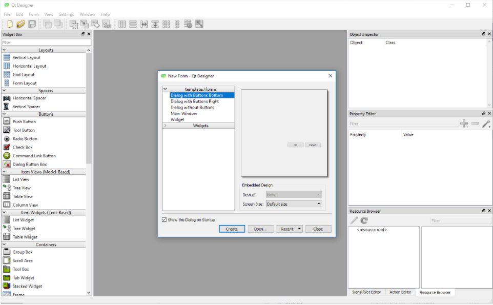
QT Designer allows for creating so-called “forms” which can be the GUI for a dialog box, a main window, or just a simple QWidget. Each form is saved as a single .ui file. To create a new form, you pick one of the templates listed in the “New Form” dialog. Go ahead and double-click the “Main Window” template. As a result, you will now see an empty main window form in the central area of the QT Designer window.
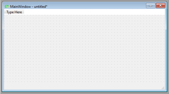
Let’s quickly go through the main windows of QT Designer. On the left side, you see the “Widget Box” pane that lists all the widgets available including layout widgets and spacers. Adding a widget to the current form can be done by simply dragging the widget from the pane and dropping it somewhere on the form. Go ahead and place a few different widgets like push buttons, labels, and line edits somewhere on the main window form. When you do a right-click in an empty part of the central area of the main window form, you can pick “Lay out” in the context menu that pops up to set the layout that should be used to arrange the child widgets. Do this and pick “Lay out horizontally” which should result in all the widgets you added being arranged in a single row. See what happens if you instead change to a grid or vertical layout. You can change the layout of any widget that contains other widgets in this way.
On the right side of QT Designer, there are three different panes. The one at the top called “Object Inspector” shows you the hierarchy of all the widgets of the current form. This currently should show you that you have a QMainWindow widget with a QWidget for its central area, which in turn has several child widgets, namely the widgets you added to it. You can pretty much perform the same set of operations that are available when interacting with a widget in the form (like changing its layout) with the corresponding entry in the “Object Inspector” hierarchy. You can also drag and drop widgets onto entries in the hierarchy to add new child widgets to these entries, which can sometimes be easier than dropping them on widgets in the form, e.g., when the parent widget is rather small.
The “Object” column lists the object name for each widget in the hierarchy. This name is important because when turning a GUI form into Python code, the object name will become the name of the variable containing that widget. So if you need to access the widget from your main code, you need to know that name and it’s a good idea to give these widgets intuitive names. To change the object name to something that is easier to recognize and remember, you can double-click the name to edit it, or you can use “Change objectName” from the context menu when you right-click on the entry in the hierarchy or the widget itself.
Below the “Object Inspector” window is the “Property Editor”. This shows you all the properties of the currently selected widget and allows you to change them. The yellow area lists properties that all widgets have, while the green and blue areas below it (you may have to scroll down to see these) list special properties of that widget class. For instance, if you select a push button you added to your main window form, you will find a property called “text” in the green area. This property specifies the text that will be displayed on the button. Click on the “Value” column for that property, enter “Push me”, and see how the text displayed on the button in the main window form changes accordingly. Some properties can also be changed by double-clicking the widget in the form. For instance, you can also change the text property of a push button or label by double-clicking it.
If you double-click where it says “Type Here” at the top, you can add a menu to the menu bar of the main window. Give this a try and call the menu “File”.
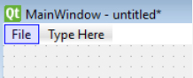
The last pane on the right side has three tabs below it. “Resource browser” allows for managing additional resources, like files containing icons to be used as part of the GUI. “Action editor” allows for creating actions for your GUI. Remember that actions are for things that can be initiated via different GUI elements. If you click the “New” button at the top, a dialog for creating a new action opens up. You can just type in “test” for the “Text” property and then press “OK”. The new action will now appear as actionTest in the list of actions. You can drag it and drop it on the File menu you created to make this action an entry in that menu.
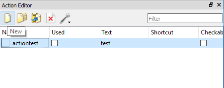
Finally, the “Signal/Slot Editor” tab allows for connecting signals of the widgets and actions created to slots of other widgets. We will mainly connect signals with event handler functions in our own Python code rather than in QT Designer, but if some widgets’ signals should be directly connected to slots of other widgets this can already be done here.
You now know the main components of QT Designer and a bit about how to place and arrange widgets in a form. We cannot teach QT Designer in detail here but we will show you an example of creating a larger GUI in QT Designer as part of the following first walkthrough of this lesson. If you want to learn more, there exist quite a few videos explaining different aspects of how to use QT Designer on the web. For now, here is a short video (12:21min) that we recommend checking out to see a few more basic examples of the interactions we briefly described above before moving on to the walkthrough.
What is goin' on everybody?
Welcome to a tutorial covering the Qtdesigner. So, up until this point, we haven't really covered much in the way of layouts because we've been manually coding everything via pyqt and idol, so we haven't really covered layouts because probably the best way to do layouts is going to be via Qtdesigner. So, it's not so much programming here, as far as the layout is concerned, but this is going to save you tons of time. So it's pretty stupid not to use it, if you ask me.
So, if you have pyqt installed and you did the full installation like I was showing you guys, you should have the Qtdesigner. Now, when you first open up the Qtdesigner, you'll have this choice here - generally, you're going to choose main window or widget.
The main window is like a main window - it comes with the main menu and stuff - so that's kind of what we want most likely but- yeah, so we'll just choose that one. And then what you're given, once it pops up, is just a simple window to work with here. And, just to talk real briefly about how the Qtdesigner is actually laid out itself, on the left hand side here you've got all the widgets, right? So you've got some layout widgets, which we haven't talked about yet, but then a bunch of other stuff like spacers, and push buttons, and checkboxes, and calendar stuff, and labels here- just basically everything, right, that- that is a part of Qt. So, these are all of our options, and it's really as simple as click and drag - bam!: you've got a button. Bam!: you've got a checkbox. Want a horizontal spacer? You got it!
So it’s a nice al-la-cart menus here. And, I don't know… let's add a label, too, while we're at it.
Okay? So, you've got all this kind of stuff- and, so what it's allowing us to do is really just do the layout aspect. So, the functionality and the code of, you know, what happens when I push a button - we still have to handle that, but the layout we do with Qtdesigner, and this is really really great because, especially when we talk about layouts here in a moment, you'll see that, if you want to deal with those, it's going take so much longer to do it manually, especially if you change your mind.
So once you have like a window kind of set up, what you can do is- obviously, like- you can kind of- I mean, this is basically the window- but if you really want to see the window - right? - like your horizontal spacer isn't going to look like that. So, what you can do is you can come to Form, and then Preview - either Preview, which is control r, or you can Preview in, and you can preview, like, the basic styles that you have access to- so you can preview like these specific things like this, or you can just control r and preview it, you know, like this. So we have this window, and, if we resize this window, though, we'll see kind of the same problem that we had had initially- is that the window- the stuff within the window doesn't resize as it ought to. So, that's what we use layouts for. So, you can apply a layout to the entire window itself by just right-clicking somewhere in open space and then coming down to layout and just choose a layout.
So you got- let's do let's do a horizontal layout, so then it’ll just give us, like, columns; so this would be column 1, column 2, 3, and 4. So let's- this divider is basically worthless, so I’m going to delete it... at least I thought I was going to delete it- Get over here! I can't- I can't seem to- there- Oh my goodness- there we go. Okay, deleted it.
Okay, so, we've got those, and then another example here is- actually let's do a layout- let's break that initial layout, and let's give this a grid layout, actually. There we go - layout and grid. Okay? So then we can, like, move things all around and it kind of shows us the valid places that we could stuff stuff.
Now, the other nice thing is you can have the entire window as a grid layout, but then you can throw in another layout like, okay, we want one of the grid spots to be a vertical layout, right, and then we can kind of- well this one isn't going to let us change the size- but then we can, okay, throw in- let's throw in a push button in there, and then let's try to stuff something else in there - see if we get away with it. Yeah. So, as you can see, this is part of that grid layout that we just built, but, then, within that grid layer- layout, we have a vertical layout as well.
So now, though, let's do control r, and we can see here, now, we can resize this, and everything resizes with it, right? And, so, that's pretty nice. So, some of the other things that we might have a problem with is, like, for example, this says text label, and this is push button, and checkbox, and all this stuff. Well, to change that, it's pretty simple - you just double-click on it, and you can put whatever you want. So we'll put 'hello there,' and then ‘push me,’ and then ‘or me,’ and then, 'but not me’ - okay? - something like that, and 'check here.' That's good enough. So, then, on this- that's kind of like this, the stuff that we have on the left-hand side here.
But, now, looking on the right-hand side, we have Object Inspector, we've got a Property Editor, which I didn't mean to move, and then we have Resource Browser. Now, I don't really use Resource Browser - not really sure what its purpose is - but Object Inspector and Property Editor are pretty useful. So, the Object Enspector - this is like for your entire window - you know, what's going on here? You've got the main window, then you've got the central widget, which is this grid layout, you've got the stuff that is within the grid layout, and they've got this new vertical layout and the stuff that's contained within it - so that's kind of the structure of the application. Then, down here, you've got the Property Editor. Depending on what you select, will show up in this Property Editor. So we could click on this button, and we get- oh it's this 'push button'- and, mainly, these are just kind of the settings. You probably won't change these very- very often, but one thing you should definitely always change is the object name. So, the object name - here's 'push-button' - this is the object name, like, in your code, so this button is defined by 'push button.' This, one 'push-button three,' this one, 'push-button two'- that's not very useful, so, before we push this to python code, we definitely want to rename these. So, maybe this one would be, you know, 'but not mel’ right, to be kind of... going along with the name of the button itself, and then we could name this one, you know, ‘push me,’ and then this one could be ‘or me,’ right? Whoops - highlighted a little too much there. ‘or me.’ Okay? So you can do stuff like that. Also, if you ever wanted to change, like, the window's title, you can't- like, you can't really click on the window and it pop-up, but you can come over to the Object Inspector, click on main window, and then you come down here to window title, and you can change the window title. So, I don't know, 'Qt type' - that's what I’ll call it. So there's that. Also, if you want to add, like, a menu, you can totally do that - just double click there, start typing stuff, right? File, open, save, let's add a separator, bam, and then ‘exit.’ Okay? Instantly done. Right? That would have taken us, like, you know, I don't know, three or four minutes to do; we just did it, like, instantly.
And then here, luckily for us, we've got Action Open, this one says Action Save, this one's Action at- Exit, so this one actually makes a little more sense automatically - you don't have to change the name - but you can if you want. So there's that.
And then, obviously, if you wanted to add more items as you, kind of, do stuff here, right, if I added 'edit' here, it gives us a new option later, you know- So, as you add more to this menu bar, it just automatically adds stuff, you know? So, if you wanted to, you could. Now how do we actually get this to python code? So, if you're on windows and you go, say, Form, View Code, you might get this error. This is, like, a known error - it makes no sense to me why this error still is in existence, but it is. So, what we want to do, if that didn't work for you, is you can go File, Save As, and we can save this. I'm going to save it in this really deep directory, in testing, and we're going to call this pyqtdesigner, and it'll be a .ui file - that's just what it's being saved as. We'll go ahead and save that, no problem. So I have that file now - it's just right in here - and, what we want to do now is open up a console in there. So, open command window into there. So, make sure you're in the actual directory of that file, right? So that's where the file is - that's the path to this file. So, if you don't know how to do that, you can always hold shift, and right-click the directory, and you can open a command window there.
So, once you've done that, now we have to enter in some code to get this to convert. So, if you- if you can, you could sometimes get away with just doing py uic - x for executable, and then we can change- we can say pyqtdesigner.ui- that's what I saved it as- yeah, and then dash O for the output file, and we're just- we'll say pyqtdesigner.py, but I don't think this will end up working for me. But it might work for you - we'll try it. Right. So, it's probably gonna come up and say it's not recognized as a command. So now we need to reference that py.uic file - it's like a batch file - so now let's reference that. So, it would be c colon slash python 34, or whatever version you're using, and then lib/ site -packages / pyqt4, or 5, or 6, or whatever is at the time that you're watching this, /piyuic4, or 5, or whatever .bat and then - same thing as before – x for executable - if you don't use the x it won't, like, actually create a window, it'll just be a bunch of definitions - you can run it but, it's not going to do anything, and then we want to do this pyqtdesigner.ui, and then we want to do the -o, and then we'll do the output to pyqtdesigner.py.
Okay? So we'll do that, hit enter, and you should now have a new file there, right? It should be pyqtdesigner. We can open it- edit with idol. Here's all that code. Again, there's no real functionality to it - it's just the layout and just the ui only - but let's go ahead and run that. And,sure enough, here's our window. And that's that. So, you've got all the python code there, you did it in the designer, obviously this isn't really any advanced code, but, hey we built that in, like, 10 minutes, so- that would have taken us a lot longer than ten minutes to build all of that including- especially thinking about, like, the layouts that are involved here- and then, like, what happens when you're like, 'hmm, I want to change layouts' - well, that's a really- kind of a challenge, especially if you have, like, a lot of stuff inside your layouts - to kind of mentally go through what objects need to be moved to what place in your code - that's pretty hard. And, so, having the Qtdesigner there just- it makes it so much simpler. So, anyways, that's just a really quick introduction to Qtdesigner. Obviously there's a whole lot more to - it this was kind of a silly application, but, from here, all we really need to do is, you know, use connect to connect functions to these buttons, but we've already covered how to do that, so I’m not going to waste any time and do these simple connections to the buttons. But, hopefully you can see, now, how powerful just Qtdesigner is, because, really, as far as I know, there's no tk designer - but maybe I’m wrong. If I’m wrong, let me know. But Qtdesigner just makes things so much easier. So, anyways, that's it for this tutorial. If you have any questions or comments, go ahead and leave them below. Otherwise, as always, thanks for watching, thanks for all the support and subscriptions, and until next time.
Once you have created the form(s) for the GUI of your program and saved them as .ui file(s), you can translate them into Python code with the help of the pyuic5 tool, e.g. by running a command like the following from the command line using the tool directly with Python :
"C:\Users\<username>\AppData\Local\ESRI\conda\envs\arcgispro-py3-clone\python.exe" –m PyQt5.uic.pyuic mainwindow.ui –o mainwindow.py
or
"C:\Program Files\ArcGIS\Pro\bin\Python\envs\arcgispro-py3\python.exe" –m PyQt5.uic.pyuic mainwindow.ui –o mainwindow.py
, depending on where your default Python environment is located (don't forget to replace <username> with your actual user name in the first version and if you get an error with this command try typing it in, not copying/pasting). mainwindow.ui, here, is the name of the file produced with QT Designer, and what follows the -o is the name of the output file that should be produced with the Python version of the GUI. If you want, you can do this for your own .ui file now and have a quick look at the produced .py file and see whether or not you understand some of the things happening in it. We will demonstrate how to use the produced .py file to create the GUI from your Python code as part of the walkthrough in the next section.
2.7 Walkthrough: Building a GUI-based tool to create features from querying web services
In this walkthrough, our main goal is to demonstrate how to build a small software application with a reasonably complex GUI in Python with the help of PyQt5 and the QT Designer. The software is supposed to work as a stand-alone application but also as a script tool inside ArcGIS Pro. Furthermore, while part of its functionality will require arcpy, we also want it to provide some functionality if arcpy is not available. Therefore, this walkthrough will also show how one can check whether a Python script is run inside ArcGIS or not, and whether arcpy is available or not. Finally, since the software will query some geographic web services that return JSON code, the walkthrough will be a continuation of what we started in Section 2.3 where you learned about Python packages that support dealing with URLs and web requests as well as working with JSON code.
Note: Unfortunately there currently is an issue with the newest versions of ArcGIS Pro (version 2.8 and above) that will make the application from this walkthrough crash when it is run as a script tool inside ArcGIS. We have not yet been able to find a workaround for this issue that does not require re-designing the GUI of the app. The issue seems to be related to specific QT5 widgets (menu bar, status bar, etc.) used in the program. You will still be able to run the software as a stand-alone application though if you have one of these versions.
2.7.1 Overview of the software tool
The idea of the little software tool we are going to build is that sometimes you would like to be able to quickly create a feature class with points for certain places based on their names. Let’s say you want to produce a shapefile showing a few places in the city you are living in. What you could do is open a basemap in ArcGIS or some other GIS software and then digitize point features for these particular locations. Or you could look up the coordinates of the places in some external application such as Google Maps and then create new point features based on these coordinates manually or by exporting the coordinates in a format that can be imported by your GIS. Both these options are relatively time consuming and require several steps. We therefore want to exploit the fact that there exist many web services that allow for querying for geographic places based on name, type, and other properties, and getting back the coordinates. The two web services we are going to work with are the Nominatim query interface to OpenStreetMaps (OSM) and the place query interface of the online geographic gazetteer GeoNames. We will discuss these services in more detail below. Our tool should allow us to enter a query term such as a place name, pick a query service and set some additional query options, and then run the query to get a list of candidate places with coordinates. We can then look at the result list and pick one or more candidates from the list and either
- add them to a layer currently open in ArcGIS Pro (assuming that the software is run as a script tool inside ArcGIS),
- add them to a shapefile on disk, or
- add the result to a CSV text file (basically an alternative that still works even when arcpy is not available).
Figure 2.20 and the video below show the GUI of the software and further illustrate how the tool works. The use case in the shown example is that we use the tool to populate a layer open in ArcGIS Pro with some of the main sightseeing locations in Paris including the Eiffel Tower, the Louvre, etc.
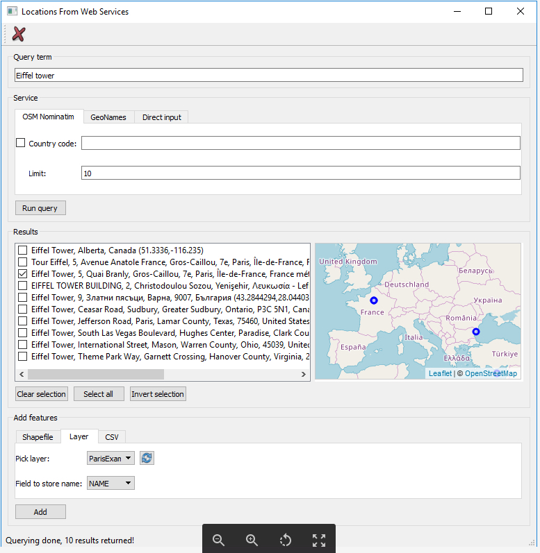
Please watch the following video, Location from Web Service Tool Overview (5:25min):
Hello. In this video, I'm quickly going to show you, or demonstrate to you, the tool that we are going to build in this walkthrough, the tools for querying different surfaces on the map to create point features, and then add them either to an open layer in ArcGIS, to a shape file on disk, or just to a CSV text file.
And you can see the tool here on the right on the screen, I'm currently running it inside of ArcGIS Pro, and I've already used it to add a few places for different attractions in Paris. And, um, so the GUI is structured into four different parts.
We have the part at the top, where the user can enter a query to a name of a place. Then we have an area where he can choose between different web services to query. Then an area where he will see the results of this query. And then an area where he can add the features he wants to from some data source.
So let's demonstrate this by querying for Eiffel Tower. And I'm going to use the Nominatim query interface to OpenStreetMap. I'm not going to use any of the options for this first query-- just pick the Run Query button. And you see that then the result lists here is updated based on what you get back from this Nominatim web service.
And we have this nice little map, which appear on the right, that shows us the different results on the map, which can also be very handy. Obviously, we are interested in the one here that is located in Paris.
So we can actually click on that one, and then see, OK, this is the one called Eiffel Tower. So, basically the third one here from our list-- so what I can do is use the buttons below the results to clear the selection, and then to say, I just want this entry here. And, here at the bottom, you can see that I'm currently on the tab for adding the features to a layer in ArcGIS Pro. And I've selected the Paris example layer that I set up for this project, and the names of the features should be stored in the field called name of that layer.
So I would just click the Add button now to add this one feature for the Eiffel Tower to this data set. And actually, for having it show up on the map, I need to zoom in and out a bit so the map gets updated. And then you see here now that this new point has been added.
And, just to show you the rest of the interface-- we have another tab here for instead of Nominatim querying the geo name step service, with different options for that. And we have also the tab that allows us for directly entering features with name, latitude, and longitude. So let's say I have created this map for a friend, and now I also want to add my home as a place to that map. I could enter it here, my home, and then I would have to enter some coordinates. So let's hope that I'm going to find something that's at least somewhere in the area of Paris.
It's still-- the button has to run code run query, but in principle it just creates a single point feature from what I entered here, that is shown here on the list. Looks like I actually at least - it's somewhere in Paris. And I can now also add that one to the layer here.
So I'm not sure which one is in the place, I think it's the one up here-- that one here. So that's now-- I can click on it, yes, that's the place, my home. So you see now that the result has indeed been added to the layer.
And just to look at the last steps here-- so the shape file tab would allow us to, instead, add the features a shape file on disk. And there's also the option to create a new shape file for that purpose that opens a separate dialog box, for which you also will have to create the graphical user interface.
And the last one is the CSV tab, where it just can select a file to which the features will be added as, basically, name, latitude, longitude columns. And the buttons with the three dots on it are always for opening a file a dialogue for selecting a particular shape file or CSV file.
OK, so much for this overview, and now we will move on to actually create the graphical user interface for this tool.
The GUI is organized into four main parts:
- The text field for entering the query term. We are currently querying for "Eiffel tower".
- The section where you pick a web query service and set some additional options. The figure shows the interface for the Nominatim OSM service. In addition to Nominatim and GeoNames, we also have a “Direct Input” tab for adding places directly by providing a name and lat/lon coordinates.
- Since the query has already been run, the "Results" section shows different candidate toponyms returned by the Nominatim service for our query. The third one looks like the result we want, so we selected just that one. The selection can be changed with the help of the buttons below or by directly checking or unchecking the checkboxes. Next to the result list is a browser widget that is used to display a Leaflet based web map of the results.
- The final section is for adding the selected features to some dataset. The figure shows the tab for adding them to a currently open layer in ArcGIS Pro.
We can run as many queries as we wish with the tool and collect the results we want to keep in one of the possible output options. While we will only present a basic version of the tool in this walkthrough supporting two different query interfaces and direct input, the tool could easily be extended to provide access to other web portals so that it can be used for running queries to, for instance, get locations of all Starbucks located in a particular city or create locations from a list of addresses.
Before we continue with exploring the GUI and code of the application, let us talk about the two web services we are going to use:
Nominatim – Surely, you know about OpenStreetMaps (OSM) and how it collects geographic data from volunteers all over the world to create a detailed map of the world. OSM data is freely available and can be directly exported from the OSM web site. In addition, there exist quite a few web services built around the OSM data, some of them created with the purpose of allowing for querying the data to only obtain information about particular features in the data. One such example is the Nominatim web service provided by OSM themselves. The website for Nominatim Open Street Maps provides an easy to use interface to the Nominatim query engine. You can type in a search term at the top and then will get to see a list of results displayed on the left side of the page and an OSM based map on the right that shows the currently selected entity from the result list. Give it a try, for instance by running a query for “Eiffel tower, France”.
Note: With some recent changes, it seems Nominatim has become much more restrictive and will often only return a single result rather than multiple options. If you leave out the 'France' in the query, the only result returned will actually not be the Eiffel Tower in Paris. However, you will still get multiple results if you, for instance, enter 'Washington' as the query string. Due to these changes, the results you will get when using Nominatim in the Locations from Web Services Tool will partially deviate from what is shown in the figures and videos in this section (for instance, the list of options shown in Figure 2.25 when only querying for 'Eiffel tower' without country name.
Nominatim provides an HTTP based web API that can be used for running queries from your own code and getting the results back, for instance as JSON or XML data. The web API is explained on this wiki page here. Query terms and additional parameters are encoded in a URL that has the general format:
https://nominatim.openstreetmap.org/search
where parameters are specified as <parameter name>=<parameter value> pairs and multiple parameters have to be separated by an & symbol. The parameter name for the query string is simply 'q' (so q=...). To run the query, the client sends an HTTP GET request with this URL to the Nominatim server who processes the query and parameters, derives the result, and sends back the results to the client. The format parameter controls how the result is presented and encoded. Without specifying that parameter, you will get the kind of HTML page that you already saw above with the result list and map. When using format=json as we will do in the following, we get the result as a list of entities encoded as JSON. Here is an example query URL, querying for “Eiffel tower, France” again, that you can test out simply by clicking on the link to open the URL in your browser:
https://nominatim.openstreetmap.org/search?q=Eiffel%20tower%2c%20France&format=json
Have a look at the result shown in your browser. As we explained at the beginning of the lesson, JSON uses [...] to denote lists of entities
[ <entity1, entity2>, ... ]
where each entity is described by its properties like in a Python dictionary:
{<property1>: <value>, <property2>: <value>, ...}
Due to the changes, we mentioned above, the result will be a list with just a single entity, looking like this ...
[{
    "place_id":115316817,
    "licence":"Data © OpenStreetMap contributors, ODbL 1.0. http://osm.org/copyright",
    "osm_type":"way",
    "osm_id":5013364,
    "lat":"48.8582599",
    "lon":"2.2945006358633115",
    "class":"man_made",
    "type":"tower",
    "place_rank":30,
    "importance":0.5868325701744196,
    "addresstype":"man_made",
    "name":"Eiffel Tower",
    "display_name":"Eiffel Tower, 5, Avenue Anatole France, Quartier du Gros-Caillou, 7th Arrondissement, Paris, Ile-de-France, Metropolitan France, 75007, France",
    "boundingbox":["48.8574753","48.8590453","2.2933119","2.2956897"]
}]
We can see that the most important properties for us will be the ‘display_name’ property and the ‘lat’ and ‘lon’ properties (appearing in bold above) in order to create point features and add them to an existing data set with our tool. Feel free to compare this result to what you get when querying for 'Washington' where you will get a list of multiple results.
The following query uses a few more parameters to query for places called London in Canada (countrycodes=CA) and asking for only a single entity be returned (limit=1).
https://nominatim.openstreetmap.org/search?q=London&format=json&countrycodes=CA&limit=1
If you look at the result, you will see that it lists London in Ontario as the only result. Without using the ‘countrycodes’ parameter the result would have been London in the UK because Nominatim uses a ranking scheme to order entities by likelihood/prominence. Without the 'limit' parameter, we would get a list of multiple options in the JSON result. ‘format’, ‘countrycodes’ and ‘limit’ will be the only parameters we will be using in our tool but please have a look at the other parameters and examples given on the Nominatim wiki page to get an idea of what other kinds of queries could be implemented.
GeoNames – You have already seen the Nominatim examples, so we can keep the section about GeoNames a bit shorter, since the URLs for running queries are somewhat similar. GeoNames is essentially an online geographic gazetteer, so a directory of geographic place names with associated information including coordinates. The main page can be used to type in queries directly but we will be using their REST web API that is documented here. Instead of a parameter for specifying the output format, the API uses a special URL for running queries that are replied to using JSON, as in the following example:
http://api.geonames.org/searchJSON?name=Springfield&maxRows=10&username=demo
Please note that a parameter (name=) is used to specify the query term. In addition, GeoNames requires a user name to be provided with the ‘username’ parameter. In case you tried out the link above, you probably got the reply that the daily request limit for user ‘demo’ has been reached. So you will have to create your own account at http://www.geonames.org/login and then use that user name instead of ‘demo’ in the query. The JSON sent back by GeoNames as the result will start like this:
{
    "totalResultsCount": 3308,
    "geonames": [
        {
            "adminCode1": "IL",
            "lng": "-89.64371",
            "geonameId": 4250542,
            "toponymName": "Springfield",
            "countryId": "6252001",
            "fcl": "P",
            "population": 116565,
            "countryCode": "US",
            "name": "Springfield",
            "fclName": "city, village,...",
            "adminCodes1": {
                "ISO3166_2": "IL"
            },
            "countryName": "United States",
            "fcodeName": "seat of a first-order administrative division",
            "adminName1": "Illinois",
            "lat": "39.80172",
            "fcode": "PPLA"
        },
        {
            "adminCode1": "MO",
            "lng": "-93.29824",
            "geonameId": 4409896,
            "toponymName": "Springfield",
            "countryId": "6252001",
            "fcl": "P",
            "population": 166810,
            "countryCode": "US",
            "name": "Springfield",
            "fclName": "city, village,...",
            "adminCodes1": {
                "ISO3166_2": "MO"
            },
            "countryName": "United States",
            "fcodeName": "seat of a second-order administrative division",
            "adminName1": "Missouri",
            "lat": "37.21533",
            "fcode": "PPLA2"
        }
    ]
}
Here the list of entities is stored under the property called ‘geonames’. Each entity in the list has the properties ‘toponymName’ with the entity name, ‘lng’ with the longitude coordinate, and ‘lat’ with the latitude coordinate. Query parameters we will be using in addition to ‘name’ and ‘username’ are ‘maxRows’ to determine the number of results sent back, ‘country’ to restrict the search to a single country, and ‘featureClass’ to look only for features of a particular type (codes A,H,L,P,R,S,T,U,V of the GeoNames feature class codes defined here).
2.7.2 Creating the GUI in QT Designer
The GUI of our software application is not too complex but still uses many of the most common GUI elements such as a toolbar with a tool button, normal push buttons, group boxes, tabs, labels, text input fields, checkboxes, combo boxes, list views, and a status bar. You already got to know most of these in Section 2.6 but there are also some new ones. The GUI consists of two parts, the GUI for the main window and the GUI for the dialog box that is shown when the user clicks on the “Create new shapefile…” button. Therefore, we will be producing two different .ui files with QT Designer called gui_main.ui and gui_newshapefile.ui. The GUI of the main window uses a vertical layout to organize the different elements into four different rows as shown in the figure below.
Each of the rows is formed by a QGroupBox widget and then other widgets are arranged hierarchically within these group boxes using a combination of grid and horizontal layouts. The tool doesn’t have a menu bar but a toolbar at the top with a button to exit the program and a status bar at the bottom. When creating the GUI in QT Designer, it will be important to name the widgets we need to refer to from our main code as indicated by the orange labels in the two figures below. As we already pointed out, the object names given to the widgets in QT Designer will be the names of the variables used for storing the widgets when the .ui file is compiled into a .py file.
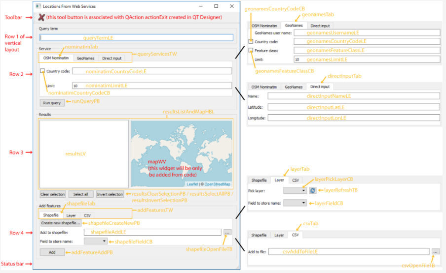
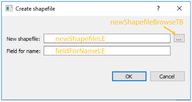
The series of videos linked below shows the process of creating the GUI in QT Designer. A zip file with the resulting .ui files is available for download here. We recommend that you work along with the video, pausing it as needed, to create the GUI yourself to get some more practice with QT Designer. The downloadable .ui files are mainly intended as a fallback position in case you experience any difficulties while creating the GUI or later on when compiling the .ui files and using the produced Python code. If you cannot replicate what is shown in the video, please ask for help on the discussion forums.
Create the GUI along with this series of videos [~45 min of video materials]
At this point, you either have saved your own two .ui files or, if you ran into any issues, will continue with these files downloaded from the link posted above. We now need to compile the files into Python code with pyuic5. We do this by running the ArcGIS Pro python.exe from the Windows command line with the pyuic module. The python.exe file is located in the folder “C:\Users \<username>\AppData\Local\ESRI\conda\envs\arcgispro-py3-clone\" (unless the ArcGIS Pro Python environment you are using is located in a different folder). So open a command shell, navigate to the folder containing the .ui files and then run the following two commands (again picking the correct version depending on where your default Python environment is installed and replacing <username> as needed):
"C:\Users\<username>\AppData\Local\ESRI\conda\envs\arcgispro-py3-clone\python.exe" –m PyQt5.uic.pyuic gui_main.ui –o gui_main.py
"C:\Program Files\ArcGIS\Pro\bin\Python\envs\arcgispro-py3\python.exe" –m PyQt5.uic.pyuic gui_main.ui –o gui_main.py
and
"C:\Users\<username>\AppData\Local\ESRI\conda\envs\arcgispro-py3-clone\python.exe" –m PyQt5.uic.pyuic gui_newshapefile.ui –o gui_newshapefile.py
"C:\Program Files\ArcGIS\Pro\bin\Python\envs\arcgispro-py3\python.exe" –m PyQt5.uic.pyuic gui_newshapefile.ui –o gui_newshapefile.py
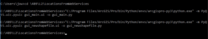
The parameters given to pyuic5 are the name of the input .ui file and then –o followed by the name of the output file. You should now have the two files gui_main.py and gui_newshapefile.py in the project folder. Let us have a quick look at the produced code. Open the produced file gui_main.py in your preferred Python IDE and see whether you recognize and understand how the different elements are created and how their properties are set. Without going into the details, the code defines a class Ui_MainWindow with a method setupUi(…). The parameter MainWindow is for passing a QMainWindow widget to the method. The rest of the code of the method then either...
- changes properties of MainWindow,
- creates new widgets and layouts storing them as attributes of the Ui_MainWindow object and sets their properties, or
- adds widgets to MainWindow or to other widgets to create the hierarchical organization of the widgets.
class Ui_MainWindow(object):

    def setupUi(self, MainWindow):
        …
        MainWindow.resize(605, 685)   # changes property of main window widget
        self.centralwidget = QtWidgets.QWidget(MainWindow) # creates child widgets and stores them in attributes of the Ui_MainWindow object
        …
        MainWindow.setCentralWidget(self.centralwidget) # adds widgets to main window
        …
This all means that we can create a new QMainWindow widget in our code with ...
mainWindow = QMainWindow()
... create an object of the UI_MainWindow class with
ui = gui_main.Ui_MainWindow()
... and then create the GUI for the main window by calling ui.setupUi(…) with mainWindow as the parameter:
ui.setupUi(mainWindow)
Whenever we need to access a widget created by setupUi(…), we can do so by using the expression
ui.<object name of the widget>
where the object name is the name we gave the widget in QT Designer, e.g.
ui.queryTermLE
for the QLineEdit widget we created for entering the query term.
2.7.3 Main code of the tool and how it works
Now we are going to develop the main code for our tool that imports the gui_main.py and gui_newshapefile.py files, sets up the application, and connects the different GUI elements with event handler functions and functions that realize the actual functionality of the tool. We will organize the code into several modules. In particular, we will keep the functions that realize the main functionality, such as querying the different web portals, creating a new shapefile, etc. in a separate Python script file called core_functions.py . These functions are completely independent of the GUI of our tool and the few global variables we will need, so we might want to use them in other projects. Separating the project cleanly into GUI dependent and GUI independent code fosters reusability of the GUI independent code. Overall, the project will consist of the following Python files:
- gui_main.py – compiled version of gui_main.ui for setting up the GUI of the main window,
- gui_newshapefile.py – compiled version of gui_newshapefile.ui for setting up the GUI of the dialog box for creating a new shapefile,
- core_functions.py – contains definitions of functions for main functionality that are completely independent of GUI and global variables
- main.py – contains the event handler functions and the code for wiring up the GUI as well as setting up and running the application
In the following, we will focus on the code from main.py but we will start with a brief look at core_functions.py, so please download the file core_functions.py and open it so that you can read the code for the different functions. Most of the functions defined in the script should be rather easy to understand from the comments in the code and from your experience with using arcpy to work with shapefiles. Here is an overview of the functions with a few additional explanations:
- queryNominatim(query, limit=10, countryCodes=''): The purpose of this function is to query the Nominatim query interface of OSM for a query string and parameters for the limit of results returned and country code for the country to search in as discussed in Section 2.7.1. The code should be easy to understand: urllib.parse(…) is used to encode the query string to be used as part of a URL, before the final query URL is put together. The get(…) method of the requests package is used to run the actual query and the returned result is translated into JSON before being returned. Since no error handling is done in this function, we will have to deal with potential exceptions raised within the function in the code that calls this function.
- queryGeonames(query, maxRows = 10, username='', country='', featureClass=''): This function does the same as queryNominatim(...) but for GeoNames and for a different set of query parameters. Since GeoNames returns JSON code with the list of candidate features stored under the attribute 'geonames', we return json['geonames'] at the end.
- getStringFieldsForDescribeObject(desc): This is the first of a few auxiliary functions for getting information from shapefiles and layers. An arcpy.Describe object of a data set needs to be passed to it and it then returns a list of all editable string fields of that layer.
- getValidFieldsForShapefile(fileName): This function is used to get a list of editable string fields for a shapefile whose name is provided as a parameter. It relies on getStringFieldsForDescribeObject(…) to do most of the work but before that checks that the shapefile exists and is a Point vector data set. If not, it will return an empty list.
- createPointWGS1984Shapefile(fileName, fieldName): This function creates a new Point shapefile with the name provided as parameter, using WGS 1984 coordinates, and with a single additional string field whose name is also provided as a parameter.
- getPointLayersFromArcGIS(): This function is for getting a list of Layer objects for the layers currently open in ArcGIS Pro but only including Point layers.
- importArcpyIfAvailable(): This function returns True if arcpy is available for import, else False. It attempts to import arcpy within a try-except construct so that, if the operation fails, the resulting exception is caught and False is returned.
- runningAsScriptTool(): This function returns True if the program is run as a script tool inside ArcGIS, else False. This is accomplished by calling arcpy.mp.ArcGISProject("CURRENT") and catching the resulting exception if this operation fails, meaning the program is run as a standalone program outside of ArcGIS.
- webMapFromDictionaryList(features): This function produces and returns the HTML code for displaying the web map as part of the GUI. It gets the features that should be displayed on the map as parameter in the form of a list of dictionaries with name, lat, and lon attributes.
Now that you know the functions we have available for realizing the different operations that we will need, let’s develop the code for main.py together. Open a new file main.py in your IDE, then follow the steps listed on the next few pages.
2.7.3.1: Step 1
We start by importing the different packages of the Python standard library and PyQt5 that we will need in this project. In addition, we import the gui_main.py and gui_newshapefile.py files so that the Ui_MainWindow and Ui_Dialog classes defined in them are available for creating the GUIs of the main window and dialog for creating a new shapefile, and of course the core_functions module. We are not importing arcpy here because we want the tool to be runnable even when arcpy is not available and that is why we defined the auxiliary function for testing its availability in core_functions.py. In addition, we are including some comments to define sections within the script for different purposes. We will fill in the code for these sections step-by-step in the following steps. At the very end, we already have the by-now-familiar code for showing the main window and starting the event processing loop of our application (even though we are not creating the application and main window objects yet).
import sys, csv

from PyQt5.QtWidgets import QApplication, QMainWindow, QStyle, QFileDialog, QDialog, QMessageBox, QSizePolicy
from PyQt5.QtGui import QStandardItemModel, QStandardItem,  QDoubleValidator, QIntValidator
from PyQt5.QtCore import QVariant
from PyQt5.Qt import Qt

try:
    from PyQt5.QtWebEngineWidgets import QWebEngineView as WebMapWidget
except:
    from PyQt5.QtWebKitWidgets import QWebView as WebMapWidget

import gui_main
import gui_newshapefile
import core_functions

# =======================================
# GUI event handler and related functions
# =======================================

#==========================================
# create app and main window + dialog GUI
# =========================================

#==========================================
# connect signals
#==========================================

#==================================
# initialize global variables
#==================================

#============================================
# test availability and if run as script tool
#============================================

#=======================================
# run app
#=======================================
mainWindow.show()
sys.exit(app.exec_())
You may be wondering what is happening in lines 8 to 10. The reason for the try-except construct there is the web view widget we are using in the "Results" part of the GUI to display a Leaflet-based web map of the results. There have been some changes with regard to the web view widget over the last versions of QT5 with the old class QWebView becoming deprecated and a new class QWebEngineView being added to replace it. The purpose of the code is to use QWebEngineView if it is available (meaning the code is run with a newer version of PyQt5) and otherwise fall back to using QWebView. The alias WebMapWidget is used to make sure that in both cases the imported class is available under the same name.
2.7.3.2: Step 2
In the next step, we add the code for creating the QApplication and the QMainWindow and QDialog objects for the main window and the dialog for creating a new shapefile with their respective GUIs. For this, please paste the following code into your script directly under the comment “# create app and main window + dialog GUI”:
app = QApplication(sys.argv)

# set up main window
mainWindow = QMainWindow()
ui = gui_main.Ui_MainWindow()
ui.setupUi(mainWindow)

ui.actionExit.setIcon(app.style().standardIcon(QStyle.SP_DialogCancelButton))
ui.layerRefreshTB.setIcon(app.style().standardIcon(QStyle.SP_BrowserReload))

ui.directInputLatLE.setValidator(QDoubleValidator())
ui.directInputLonLE.setValidator(QDoubleValidator())
ui.nominatimLimitLE.setValidator(QIntValidator())
ui.geonamesLimitLE.setValidator(QIntValidator())

mapWV = WebMapWidget()
mapWV.page().profile().setHttpAcceptLanguage("en-US")
mapWV.setHtml(core_functions.webMapFromDictionaryList([]))
ui.resultsListAndMapHBL.addWidget(mapWV)
mapWV.setFixedSize(300,200)
mapWV.setSizePolicy(QSizePolicy(QSizePolicy.Fixed,QSizePolicy.Fixed))

# set up new shapefile dialog
createShapefileDialog = QDialog(mainWindow)
createShapefileDialog_ui = gui_newshapefile.Ui_Dialog()
createShapefileDialog_ui.setupUi(createShapefileDialog)
In lines 4 to 6, we are creating the mainWindow object and then its GUI by calling the ui.SetupUi(…) method of an object we created from the Ui_MainWindow class defined in gui_main.py. The same happens in lines 23 to 25 for the dialog box for creating a new shapefile. The rest of the code is for creating some additional elements or setting some properties of GUI elements that we couldn’t take care of in QT Designer:
- Lines 8 and 9: Here we set the icons for the exit and refresh tool buttons in the GUI taking icons from the QT standard icon set.
- Lines 11 to 14: What happens here is something that we did not discuss before. QT provides some way to set up so-called Validator objects for determining what the user is allowed to enter into a line edit widget. We use QDoubleValidator and QIntValidator objects to restrict the input for Latitude and Longitude widgets of the “Direct Input” tab to floating point numbers and for the Limit widgets of the Nominatim and GeoNames query tabs to integer numbers, respectively.
- Line 16 to 20 are for creating the web view widget next to the list view widget in the third row of our main window layout. Remember how we explained in the previous section that we are defining the name WebMapWidget as an alias for the web widget that is available in the version of PyQt5 that is being used. In QT Designer, we created a QHBoxLayout for this row which is now accessible in ui.resultsListAndMapHBL, so we add the new widget to that layout and make some changes to its layout related attributes to give the widget a constant size that matches the size of the web map produced by the function webMapFromDictionaryList(…) from the core_functions.py module.
- At this point, you can actually run the code and it should already produce the desired GUI for the main window. You just won’t be able to do much with it, since we have not defined any event handlers yet.
2.7.3.3: Step 3
We now add some code to initialize some global variables that we will need. Please add the following code directly under the comment “# initialize global variables”:
# dictionary mapping tabs from services tab widget to event handler functions
queryHandler = { ui.nominatimTab: runNominatimQuery, ui.geonamesTab: runGeonamesQuery, ui.directInputTab: runDirectInput }

# dictionary mapping tabs from add feature tab widget to event handler functions
addFeaturesHandler = { ui.layerTab: addFeaturesToLayer, ui.shapefileTab: addFeaturesToShapefile, ui.csvTab: addFeaturesToCSV }

result = []                     # global variable for storing query results as list of dictionaries
arcValidLayers= {}              # dictionary mapping layer names to layer objects

arcpyAvailable = False          # indicates whether is available for import
runningAsScriptTool = False     # indicates whether script is run as script tool inside ArcGIS
The first two variables defined, queryHandler and addFeaturesHandler, are dictionaries that contain the information of which event handler functions should be called when the “Run query” button and “Add features” button are clicked, respectively, depending on which of the tabs of the two different tab widgets are currently selected. Line 2, for instance, says that if currently the tab ui.nominatimTab is open in the Services section, then the function runNominatimQuery(…) should be called. So far we have not defined that function yet, hence, you will not be able to run the program at the moment but it shows you that functions in Python are treated like other kinds of objects, meaning they can, for instance, be stored in a dictionary. You will hear more about this in Lesson 3.
The other global variables we define in this piece of code are for keeping track of the results currently displayed in the Results list view widget of our GUI, of the currently open Point layers in ArcGIS when being run as a script tool, of whether the arcpy module is available, and of whether the program is being run as a script tool or not. We will add code to initialize the last two of these variables correctly in a moment
2.7.3.4: Step 4
To now initialize the variables arcpyAvailable and runningAsScriptTool correctly and potentially disable some GUI elements, please add the following code directly under the comment “# test availability and if run as script tool”:
arcpyAvailable = core_functions.importArcpyIfAvailable()

if not arcpyAvailable:
    ui.addFeaturesTW.setCurrentWidget(ui.csvTab)
    ui.addFeaturesTW.setTabEnabled(ui.addFeaturesTW.indexOf(ui.shapefileTab),False)
    ui.addFeaturesTW.setTabEnabled(ui.addFeaturesTW.indexOf(ui.layerTab),False)
    ui.statusbar.showMessage('arcpy not available. Adding to shapefiles and layers has been disabled.')
else:
    import arcpy
    if core_functions.runningAsScriptTool():
        runningAsScriptTool = True
        updateLayers()
    else:
        ui.addFeaturesTW.setTabEnabled(ui.addFeaturesTW.indexOf(ui.layerTab),False)
        ui.statusbar.showMessage(ui.statusbar.currentMessage() + 'Not running as a script tool. Adding to layer has been disabled.')
What happens here is that we first use importArcpyIfAvailable() from the core_functions module to check whether we can import arcpy. If this is not the case, we make the “CSV” tab the current and only selectable tab from the Add Features tab widget by disabling the “Shapefile” and “Layer” tabs. In the else-part (so if arcpy is available), we further use the runningAsScriptTool() function to check if the program is being run as a script tool inside ArcGIS. If not, we just disable the “Layer” tab and make the “Shapefile” tab the currently selected one. In addition, some warning message in the statusbar is produced if either the “Layer” or both the “Layer” and “Shapefile” tabs had to be disabled.
2.7.3.5: Step 5
Time to get back to the GUI and implement the required event handler functions for the different GUI elements, in particular the different buttons. This will be quite a bit of code, so we will go through the event handler functions individually. Please add each function in the order they are listed below to the section labeled “# GUI event handler and related functions”:
# query and direct input functions

def runQuery():
    """run one of the different query services based on which tab is currently open"""
    queryString = ui.queryTermLE.text()
    activeTab = ui.queryServicesTW.currentWidget()
    queryHandler[activeTab](queryString)   # call a function from the dictionary in queryHandler
This is the event handler function for when the “Run query” button is clicked. We already mentioned the global variable queryHandler that maps tab widgets to functions. So we here first get the text the user entered into the queryTermLE widget, then get the currently selected tab from the queryServicesTW tab widget, and finally in the last line we call the corresponding function for querying Nominatim, GeoNames, or providing direct input. These functions still need to be defined.
def setListViewFromResult(r):
    """populate list view with checkable entries created from result list in r"""
    m = QStandardItemModel()
    for item in r:
        item = QStandardItem(item['name'] + ' ('+item['lat'] + ',' + item['lon'] + ')')
        item.setFlags(Qt.ItemIsUserCheckable | Qt.ItemIsEnabled)
        item.setData(QVariant(Qt.Checked), Qt.CheckStateRole)
        m.appendRow(item)
    ui.resultsLV.setModel(m)
setListViewFromResult(…) is an auxiliary function for populating the resultsLV list view widget with the result from a query or a direct input. It will be called from the functions for querying the different web services or providing direct input that will be defined next. The given parameter needs to contain a list of dictionaries with name, lat, and lon properties that each represent one item from the result. The for-loop goes through these items and creates list items for the QStandardItemModel from them. Finally, the resulting model is used as the list model for the resultsLV widget.
def runNominatimQuery(query):
    """query nominatim and update list view and web map with results"""
    ui.statusbar.showMessage('Querying Nominatim... please wait!')

    country = ui.nominatimCountryCodeLE.text() if ui.nominatimCountryCodeCB.isChecked() else ''
    limit = ui.nominatimLimitLE.text()

    try:
        items = core_functions.queryNominatim(query, limit, country) # run query
        # create result list from JSON response and store in global variable result
        global result
        result = [(lambda x: {'name': x['display_name'],'lat': x['lat'], 'lon': x['lon']})(i) for i in items]
        # update list view and map with results
        setListViewFromResult(result)
        mapWV.setHtml(core_functions.webMapFromDictionaryList(result))
        ui.statusbar.showMessage('Querying done, ' + str(len(result)) + ' results returned!')
    except Exception as e:
        QMessageBox.information(mainWindow, 'Operation failed', 'Querying Nominatim failed with '+ str(e.__class__) + ': ' + str(e), QMessageBox.Ok )
        ui.statusbar.clearMessage()
This is the function that will be called from function runQuery() defined above when the currently selected “Service” tab is the Nominatim tab. It gathers the required information from the line edit widgets on the Nominatim query tab, taking into account the status of the corresponding checkboxes for the optional elements (using the "... if ... else ..." ternary operator). Then it calls the queryNominatim(…) function from the core_functions module to perform the actual querying (line 9) and translates the returned JSON list into a result list of dictionaries with name, lat, and lon properties that will be stored in the global variable result. Note that we are using list comprehension here to realize this translation of one list into another. The resultLV list view and mapWV web map widget will then be updated accordingly. This happens inside a try-except block to catch exceptions when something goes wrong with querying the web service or interpreting the results. Statusbar messages are used to keep the user informed about the progress and a message box is shown if an exceptions occurs to inform the user.
def runGeonamesQuery(query):
    """query geonames and update list view and web map with results"""
    ui.statusbar.showMessage('Querying GeoNames... please wait!')

    username = ui.geonamesUsernameLE.text()
    country = ui.geonamesCountryCodeLE.text() if ui.geonamesCountryCodeCB.isChecked() else ''
    fclass = ui.geonamesFeatureClassLE.text() if ui.geonamesFeatureClassCB.isChecked() else ''
    limit = ui.geonamesLimitLE.text()

    try:
        items = core_functions.queryGeonames(query, limit, username, country, fclass ) # run query
        # create result list from JSON response and store in global variable result
        global result
        result  = [(lambda x: {'name': x['toponymName'],'lat': x['lat'], 'lon': x['lng']})(i) for i in items]
        # update list view and map with results
        setListViewFromResult(result)
        mapWV.setHtml(core_functions.webMapFromDictionaryList(result))
        ui.statusbar.showMessage('Querying done, ' + str(len(result)) + ' results returned!')
    except Exception as e:
        QMessageBox.information(mainWindow, 'Operation failed', 'Querying GeoNames failed with '+ str(e.__class__) + ': ' + str(e), QMessageBox.Ok)
        ui.statusbar.clearMessage()
This function that will be called from runQuery() if the currently selected “Service” tab is the GeoNames tab works exactly like the previous function for Nominatim, just the query parameters extracted in lines 5 to 8 are different and the translation into a result list looks a little bit different because GeoNames uses other property names ("toponymName" instead of "display_name" and "lng" instead of "lon").
def runDirectInput(query):
    """create single feature and update list view and web map with results"""
    name = ui.directInputNameLE.text()
    lon = ui.directInputLonLE.text()
    lat = ui.directInputLatLE.text()

    # create result list with single feature and store in global variable result
    global result
    result = [{ 'name': name, 'lat': lat, 'lon': lon }]
    # update list view and map with results
    setListViewFromResult(result)
    mapWV.setHtml(core_functions.webMapFromDictionaryList(result))
    ui.statusbar.showMessage('Direct input has been added to results list!')
This function will be called from runQuery() if the currently selected “Service” tab is the Direct Input tab. Again, we are collecting the relevant information from the input widgets (line 3 to 5) but here we directly produce the result consisting of just a single item (line 9). The rest works in the same way as in the previous two functions.
These were the functions required for the query section of our tool. So we can now move on to the Results section where we just need the three event handler functions for the three buttons located below the list view widget.
# list view selection functions

def selectAll():
    """select all items of the list view widget"""
    for i in range(ui.resultsLV.model().rowCount()):
        ui.resultsLV.model().item(i).setCheckState(Qt.Checked)

def clearSelection():
    """deselect all items of the list view widget"""
    for i in range(ui.resultsLV.model().rowCount()):
        ui.resultsLV.model().item(i).setCheckState(Qt.Unchecked)

def invertSelection():
    """invert current selection of the list view widget"""
    for i in range(ui.resultsLV.model().rowCount()):
        currentValue = ui.resultsLV.model().item(i).checkState()
        ui.resultsLV.model().item(i).setCheckState(Qt.Checked if currentValue == Qt.Unchecked else Qt.Unchecked)
These three functions all work very similarly: We go through all items in the list model underlying the resultsLV list view widget. In selectAll(), the check state of each item is set to “Checked”, while in clearSelection() it is set to “Unchecked” for each item. In invertSelection(), we take the item’s current state and either change it from “Checked” to “Unchecked” or vice versa (using the ternary "... if ... else ..." operator once more).
# adding features functions

def addFeatures():
    """run one of the different functions for adding features based on which tab is currently open"""
    activeTab = ui.addFeaturesTW.currentWidget()
    addFeaturesHandler[activeTab]() # call a function from the dictionary in addFeatureHandler
We have now arrived at the last row of our main window graphical interface for adding the selected result features to a layer, shapefile, or csv file. The addFeatures() function corresponds to the runQuery() function from the beginning in that it invokes the right function depending on which tab of the addFeaturesTW tab widget is currently selected. This is based on the global variable addFeaturesHandler that map tabs to functions.
def updateShapefileFieldCB():
    """update shapefileFieldCB combo box with field names based on shapefile name"""
    ui.shapefileFieldCB.clear()
    fileName = ui.shapefileAddLE.text()
    ui.shapefileFieldCB.addItems(core_functions.getValidFieldsForShapefile(fileName))
updateShapefileFieldCB() is an auxiliary function for updating the content of the shapefileFieldCB combo box whenever the name of the shapefile in the shapefileAddLE line edit widget changes so that the combo always displays the editable string fields of that shapefile.
def selectShapefile():
    """open file dialog to select exising shapefile and if accepted, update GUI accordingly"""
    fileName, _ = QFileDialog.getOpenFileName(mainWindow,"Select shapefile", "","Shapefile (*.shp)")
    if fileName:
        ui.shapefileAddLE.setText(fileName)
        updateShapefileFieldCB()
When the shapefileOpenFileTB tool button is clicked, we want to display a file dialog for picking the shapefile. Opening the dialog and processing the result happens in the function selectShapefile(). When a file name is returned (meaning the dialog wasn’t cancelled by the user), the name is put into the shapefileAddLE line edit field and updateShapefieldCB() is called to update the combo box with the field names of that file.
def addFeaturesToShapefile():
    """add selected features from list view to shapefile"""
    fieldName = ui.shapefileFieldCB.currentText()
    fileName = ui.shapefileAddLE.text()
    ui.statusbar.showMessage('Adding entities has started... please wait!')

    try:
        with arcpy.da.InsertCursor(fileName, ("SHAPE@",fieldName)) as cursor:
           for i in range(ui.resultsLV.model().rowCount()): # go through all items in list view
               if ui.resultsLV.model().item(i).checkState() == Qt.Checked:
                   point = arcpy.Point( result[i]['lon'], result[i]['lat'])
                   cursor.insertRow( (point, result[i]['name'][:30]) ) # name shortened to 30 chars
        ui.statusbar.showMessage('Adding entities has finished.')
    except Exception as e:
        QMessageBox.information(mainWindow, 'Operation failed', 'Writing to shapefile failed with '+ str(e.__class__) + ': ' + str(e), QMessageBox.Ok )
        ui.statusbar.clearMessage()
This function contains the code for writing the selected features from the results list in global variable result to the shapefile with the help of an arcpy insert cursor. We first read the relevant information from the shapefileAddLE and shapefileFieldCB widgets and then in the for-loop go through the items in the resultsLV list view to see whether they are checked or not. If an item is checked, an arcpy.Point object is created from the corresponding dictionary in variable result and then written to the shapefile together with the name of the location. Statusbar messages are used to inform on the progress or a message box will be shown if an exception occurs while trying to write to the shapefile.
def updateLayerFieldCB():
    """update layerFieldCB combo box with field names based on selected layer"""
    ui.layerFieldCB.clear()
    layer = ui.layerPickLayerCB.currentText()

    try:
        ui.layerFieldCB.addItems(core_functions.getStringFieldsForDescribeObject(arcpy.Describe(arcValidLayers[layer])))
    except Exception as e:
        QMessageBox.information(mainWindow, 'Operation failed', 'Obtaining field list failed with '+ str(e.__class__) + ': ' + str(e), QMessageBox.Ok )
        ui.statusbar.clearMessage()
This is the corresponding function to updateShapefileFieldCB() but for the layerFieldCB combo box widget part of the Layer tab.
def updateLayers():
    """refresh layers in global variable arcValidLayers and layerPickLayerCB combo box"""
    layers = []
    global  arcValidLayers
    arcValidLayers = {}
    ui.layerPickLayerCB.clear()
    ui.layerFieldCB.clear()

    try:
        layers = core_functions.getPointLayersFromArcGIS() # get all point layers
        for l in layers:                                   # add layers to arcValidLayers and GUI
            arcValidLayers[l.name] = l
            ui.layerPickLayerCB.addItem(l.name)
            updateLayerFieldCB()
    except Exception as e:
        QMessageBox.information(mainWindow, 'Operation failed', 'Obtaining layer list from  ArcGIS failed with '+ str(e.__class__) + ': ' + str(e), QMessageBox.Ok )
        ui.statusbar.clearMessage()
        ui.shapefileFieldCB.clear()
This function is for populating the layerPickLayerCB and arcValidLayer global variable with the Point vector layers currently open in ArcGIS. It uses the getPointLayersFrom ArcGIS() function from core_functions.py to get the list of layers and then in the for-loop stores the layer objects under their layer name in the arcValidLayers dictionary and just the names as items in the combo box. If something goes wrong with getting the layers from ArcGIS, the corresponding exception will be caught and a message box will warn the user about the failure of the operation.
def addFeaturesToLayer():
    """add selected features from list view to layer"""
    layer = ui.layerPickLayerCB.currentText();
    fieldName = ui.layerFieldCB.currentText()
    ui.statusbar.showMessage('Adding entities has started... please wait!')

    try:
        with arcpy.da.InsertCursor(arcValidLayers[layer], ("SHAPE@",fieldName)) as cursor:
            for i in range(ui.resultsLV.model().rowCount()): # go through all items in list view
                if ui.resultsLV.model().item(i).checkState() == Qt.Checked:
                    point = arcpy.Point( float(result[i]['lon']), float(result[i]['lat']))
                    cursor.insertRow( (point, result[i]['name'][:30]) ) # name shortened to 30 chars
        ui.statusbar.showMessage('Adding entities has finished.')
    except Exception as e:
        QMessageBox.information(mainWindow, 'Operation failed', 'Writing to layer failed with '+ str(e.__class__) + ': ' + str(e), QMessageBox.Ok )
        ui.statusbar.clearMessage()
This is the analogous function to the previously defined function addFeaturesToShapefile() but for a currently open layer and based on the information in the widgets of the Layer tab.
def selectCSV():
    """open file dialog to select exising csv/text file and if accepted, update GUI accordingly"""
    fileName, _ = QFileDialog.getOpenFileName(mainWindow,"Select CSV file", "","(*.*)")
    if fileName:
        ui.csvAddToFileLE.setText(fileName)
Similarly to selectShapefile(), this function opens a file dialog to select a csv file to append the features to.
def addFeaturesToCSV():
    """add selected features from list view to csv/text file"""
    fileName = ui.csvAddToFileLE.text()
    ui.statusbar.showMessage('Adding entities has started... please wait!')

    try:
        with open(fileName, 'a', newline='') as csvfile:
             csvWriter = csv.writer(csvfile)
             for i in range(ui.resultsLV.model().rowCount()): # go through all items in list view
                if ui.resultsLV.model().item(i).checkState() == Qt.Checked:
                     csvWriter.writerow( [ result[i]['name'], result[i]['lon'], result[i]['lat'] ])
        ui.statusbar.showMessage('Adding entities has finished.')
    except Exception as e:
        QMessageBox.information(mainWindow, 'Operation failed', 'Writing to csv file failed with '+ str(e.__class__) + ': ' + str(e), QMessageBox.Ok )
        ui.statusbar.clearMessage()
Working similarly to addFeaturesToShapefile() and addFeaturesToLayer(), this function writes the selected features as rows to a text file using the csv.writer class from the csv module of the Python standard library.
def selectNewShapefile():
    """open file dialog to creaete new shapefile and if accepted, update GUI accordingly"""
    fileName, _ = QFileDialog.getSaveFileName(mainWindow,"Save new shapefile as", "","Shapefile (*.shp)")
    if fileName:
        createShapefileDialog_ui.newShapefileLE.setText(fileName)
The final two functions are for creating a new shapefile. selectNewShapefile() is called when the newShapefileBrowseTB button that is part of the dialog box for creating a new shapefile is clicked and displays a file dialog for saving a file under a new name. The chosen name is used to set the text of the newShapefileBrowseTB line edit widget.
def createNewShapefile():
    """create new shapefile and adds field based on info in dialog GUI"""
    if createShapefileDialog.exec_() == QDialog.Accepted:
        file = createShapefileDialog_ui.newShapefileLE.text()
        field = createShapefileDialog_ui.fieldForNameLE.text()

        try:
            core_functions.createPointWGS1984Shapefile(file,field)
            ui.shapefileAddLE.setText(file)
            updateShapefileFieldCB()
            ui.shapefileFieldCB.setCurrentIndex(ui.shapefileFieldCB.findText(field))
            ui.statusbar.showMessage('New shapefile has been created.')
        except Exception as e:
            QMessageBox.information(mainWindow, 'Operation failed', 'Creating new shapefile failed with '+ str(e.__class__) + ': ' + str(e), QMessageBox.Ok )
            ui.statusbar.clearMessage()
            ui.shapefileFieldCB.clear()
This function is called when the “Create new shapefile” button on the Shapefile tab is clicked. It first displays the createShapefileDialog dialog box modally by calling its exec_() method. If the dialog is accepted (= closed by clicking Ok), the function creates the new shapefile with the help of the createPointWGS1984Shapefile() function from core_functions.py and based on the input fields in the dialog box for creating a new shapefile (newShapefileLE and fieldForNameLE). If no exception is raised, the file name and field name from the dialog box will be used to change the text of the shapefileAddLE line edit widget and the shapefileFieldCB combo box.
2.7.3.6: Step 6
At this point, we are almost done. The last thing that has to happen is connecting the widgets’ relevant signals to the corresponding slots or event handler functions. For this, please add the following code under the comment “# connect signals”:
ui.runQueryPB.clicked.connect(runQuery)
ui.resultsClearSelectionPB.clicked.connect(clearSelection)
ui.resultsSelectAllPB.clicked.connect(selectAll)
ui.resultsInvertSelectionPB.clicked.connect(invertSelection)
ui.shapefileOpenFileTB.clicked.connect(selectShapefile)
ui.addFeatureAddPB.clicked.connect(addFeatures)
ui.shapefileCreateNewPB.clicked.connect(createNewShapefile)
ui.csvOpenFileTB.clicked.connect(selectCSV)
ui.layerRefreshTB.clicked.connect(updateLayers)
ui.shapefileAddLE.editingFinished.connect(updateShapefileFieldCB)
ui.layerPickLayerCB.activated.connect(updateLayerFieldCB)

createShapefileDialog_ui.newShapefileBrowseTB.clicked.connect(selectNewShapefile)
Lines 1 to 9 and line 13 all connect “clicked” signals of different buttons in our GUI to the different event handler functions defined previously and should be easy to understand. In line 10, the “editingFinished” signal of the text field for entering the name of a shapefile is connected with the updateShapefileFieldCB() function so that, whenever the name of the shapefile is changed, the list of the fields in the combo box is updated accordingly. In line 11, we connect the “activated” signal of the combo box for selecting a layer with the upateLayerFields() function. As a result, the second combo box with the field names will be updated whenever the layer selected in the first combo box on the Layer tab is changed.
That’s it. The program is finished and can be tested and used either as a standalone application (writing features either to a shapefile or to a .csv file) or as an ArcGIS script tool. Give it a try yourself and think about which parts of the code are being executed when performing different operations. In case you want to run it as a script tool inside ArcGIS Pro, setting up the script tool for it should be straightforward. You just have to create a new script tool without specifying any parameters and provide the path to the main.py script for the source. If you have any problems running the code with your own script, the entire code can be downloaded via this link to the Locations from Web Services Complete zip file. If something in the code above is unclear to you, please ask about it on the course forums.
Obviously, the tool is still somewhat basic and could be extended in many ways including:
- providing more query options for the currently implemented query services
- incorporating other web services
- allowing for multiple query terms as input (e.g. list of place names or addresses); it could also be useful to be able to paste some longer text into the tool and then highlight place names in the text that should be queried
- supporting other geometries, not just points
- … (add your own ideas to the list)
Moreover, while we included some basic error handling with try-except, the program is not completely bullet proof and in some cases it would be desirable to provide more direct and specific feedback to the user, for instance if the user enters something into the feature class field of the GeoNames query tab that is not a valid feature class code. We are also quietly assuming that the shapefile or layer we are adding to is using a WGS1984 geographical coordinate system. Adding reprojection of the input features to the CRS of the destination would certainly be a good thing to do.
Still, the tool can be useful for creating point feature classes of locations of interest very quickly and in a rather convenient way. More importantly, this walkthrough should have provided you with a better understanding of how to create Python programs with a GUI by roughly separating the code into a part for setting up the GUI elements, a part for realizing the actual functionality (in this case the part defining the different event handler functions (GUI dependent) with the help of the core functions from core_functions.py (GUI independent)), and a part that makes the connection between the other two parts based on GUI events. You will practice creating GUIs and PyQt5 based Python programs yourself in this lesson’s homework assignment and also again in lesson 4. But for now, we will continue with looking at another aspect of creating and publishing Python applications, namely that of package management and packaging Python programs so that they can easily be shared with others.
2.8 Packages
You have already used a number of packages in Python, primarily the arcpy package, but you are likely to have encountered others, such as sys, csv, which are a part of the Python standard library, or perhaps numpy and matplotlib, which are auxiliary libraries. In the previous section of this lesson, you learned about the tkinter and PyQT libraries as we built a Python graphical User Interface (GUI). In order to use these packages you had to use the import statement to make the additional methods they provide available to your code, for example:
import arcpy
You also created modules of your own that you imported into other scripts. You simply constructed a .py file and used the import statement in order to use it, and that is all Python requires for a module to be created. Creating such a module is straightforward - all your code was contained in a single .py file, you placed the file in the same folder as the program that would use it, and you imported into that program and used its functions. You may be wondering how a module is different from a package, since they are imported the same way. The difference is that a package is a collection of modules set up for easier distribution. While some projects may consist of one simple module, you will find that if you are building a project of any complexity, more than one .py file will be required, and potentially other files as well, such as configuration files or images.
In the next section, we will look at what exactly can be imported into Python. Later in the lesson, we will demonstrate the pip and conda package and environment managers as well as the Anaconda Python distribution based on conda. The section contains several optional subsections in which we package the Locations From Web Services application from the walkthrough and upload it to distribution sites. As in Lesson 1, we recommend that you only perform what is described in these optional sections yourself if you have time left at the end of the lesson.
2.8.1 Packages and the import statement
As was mentioned earlier, when you use the import statement you can import a single .py file. In addition, the import statement can point to a folder containing a set of .py files, or a library written in a different programming language, such as C++.
You may be wondering how Python finds the module or package you specified since you only specify the name. Your own modules may have been in the current directory with the program using it, but arcpy, for example, isn’t. What happens is that Python has a list of locations that it uses in order to find the necessary packages. It traverses the list in the specific order, and, once it finds all the packages it needs, it stops looking. Here is the search order1 that Python uses:
- The home directory where the currently executing .py file is located
- PYTHONPATH directories: PYTHONPATH is a variable that is optionally set in the operating system. For example, on a Windows machine you would set it in Environmental Variables in System Settings.
- Standard library directories: The location where all standard libraries are installed on the local machine – if you have ArcGIS 10.6 Desktop installed to a default location the standard libraries can be found at C:\Python27\ArcGIS10.6\Lib. Browse to the folder, and take a quick look of all the packages that are installed.
- The contents of any .pth files: These are text files that can be created to add additional library paths; this option is used by ArcGIS Desktop 10.6. In a standard installation you can find the .pth file at C:\Python27\ArcGIS10.6\Lib\site-packages\Desktop10.6.pth. ArcGIS pro has its own .pth file: C:\Users\<username>\AppData\Local\ESRI\conda\envs\arcgispro-py3-clone\Lib\site-packages\ArcGISPro.pth or C:\Program Files\ArcGIS\Pro\bin\Python\envs\arcgispro-py3\Lib\site-packages\ArcGISPro.pth depending on your version of Pro.
- The site-package home or third-party extensions: Packages placed in Libs\site-packages directory. In a standard install of ArcGIS 10.6 Desktop that would be in the C:\Python27\ArcGIS10.6\Lib\site-packages folder.
Because of the way Python finds the code it needs to import, you need to be careful how you name your modules and packages, and where you place them. For example, if you were to create an arcpy.py module and put it in the home directory, the ArcGIS arcpy package would not be loaded.
This list above may look intimidating, but the good news is that packages you are likely to need will be packaged with special Python utilities (either pip or conda) and thus setup to place themselves in the appropriate paths without any manual intervention on your part, beyond the installation step. The other good news is that both pip and conda are fairly straightforward to use when it comes to installing packages and managing Python environments. Creating your own pip or conda packages can be a bit more involved though as you will also see in this section but still provides a convenient way for deploying and sharing your own Python applications.
1Mark Lutz: Learning Python, 5th Edition
2.8.2 Python Package Management
There are many Python packages available for use, and there are a couple of different ways to effectively manage (install, uninstall, update) packages. The two package managers that are commonly used are pip and conda. In the following sections, we will discuss each of them in more detail. At the end of the section, we will discuss the merits of the two tools and make recommendations for their use.
We will be doing some more complicated technical "stuff" here so the steps might not work as planned because everyone’s PC is configured a little differently. If you get stuck please check in with the instructor sooner rather than later. A quick troubleshooting / debugging process can involve testing to see if running the command or Command Prompt as Administrator resolves the issue, trying the Windows Command prompt instead of the Python Command prompt (or vice versa), and, if none of that has helped, trying the tech support staple of restarting your PC.
2.8.2.1 Pip
As already mentioned, pip is a Python package manager. It allows for an easier install, uninstall and update of packages. Pip comes installed with Python, and if you have multiple versions of Python you will have a different version of pip for each. To make sure we are using the version of pip that comes installed with ArcGIS Pro, we will go to the directory where pip is installed. Go to the Windows Start Menu and open the Python Command Prompt as before.
In the command window that now opens, you will again be located in the default Python environment folder of your ArcGIS Pro installation. For newer versions of Pro this will be C:\Users\<username>\AppData\Local\ESRI\conda\envs\arcgispro-py3-clone\. Pip is installed in the Scripts subfolder of that location, so type in:
cd Scripts
Now you can run a command to check that pip is in the directory – type in:
dir pip.*
The resulting output will show you all occurrences of files that start with pip. in the current folder, in this case, there is only one file found – pip.exe.
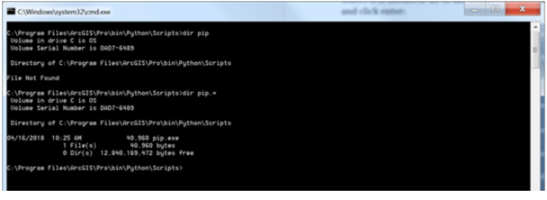
Next, let’s run our first pip command, type in:
pip --version
The output shows you the current version of pip. Pip allows you to see what packages have been installed. To look at the list type in:
pip list
The output will show (Figure 31) the list of packages and their respective versions.
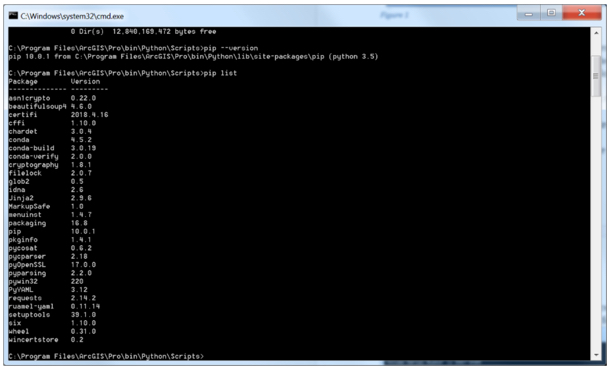
To install a package, you run the pip command with the install option and provide the name of the package, for example, try:
pip install numpy
Pip will run for a few seconds and show you a progress bar as it is searching for the numpy package online and installing it. When you run pip install, the packages are loaded from an online repository named PyPI, short for Python Package Index. You can browse available packages at Python's Package Index page. If the installation has been successful you will see a message stating the same, which you can confirm by running pip list again.
In order to find out if any packages are outdated you can run the pip list with the outdated option:
pip list –-outdated
If you find that there are packages you want to update, you run the install with the upgrade option, for example:
pip install numpy –-upgrade
This last command will either install a newer version of numpy or inform you that you already have the latest version installed.
If you wanted to uninstall a package you would run pip with the uninstall option, for example:
pip uninstall numpy
You will be asked to confirm that you want the package uninstalled, and, if you do (better not to do this or you will have to install the package again!), the package will be removed.
The packages installed with pip are placed in the Lib\site-packages folder of the Python environment you are using. You will recall that that was one of the search locations Python uses in order to find the packages you import.
2.8.2.2 Optional complementary materials: Building a pip package
Important note: While knowing how to create packages from your Python code to disseminate it is an important skill for a Python programmer, the procedure described in this section is a bit complex and error-prone due to system and installation differences. It is also not required to have performed these steps successfully yourself to finish the lesson and the rest of the course. Therefore, this section is provided for interest only. We recommend that you just read through it or skip over it completely and you can then loop back to it at the end of the lesson if you have free time or after the end of the class. If you decide to go through the steps yourself and find yourself stuck with some errors, please feel free to ask about them on the course forums but don't let such issues keep you from reading through the rest of the section and finishing the lesson.
Now that we covered the basic operation of pip, we will create a pip package for the Locations From Web Services you developed in this lesson. Creating the pip package will involve the following steps:
- Creating a __init__.py file
- Creating a setup.py file
- Installing the package
- Creating a source distribution
- Creating an account on PyPI (you need to set up an account only once)
- Publishing the package and the source to PyPI
We will walk through all these steps and create the necessary files and folders. For reference, as you are reading on, your final package folder and file structure should look like this for pip:
<yourinitialsdate>locationsfromwebservices
├── setup.py
└── <yourinitialsdate>locationsfromwebservices
   ├── __init__.py
   ├── core_function.py
   ├── gui_main.py
   ├── gui_main.ui
   ├── gui_newshapefile.py
   ├── gui_newshapefile.ui
   └── main.py
Let’s start by creating a separate folder and copying the existing code files into it. Create a pip directory in a location of your choice. Then create a folder named <yourinitialsdate>locationsfromwebservices within it. Replace the <yourinitialsdate> part of the folder name with the combination of your initials and current date and leave out the <>. From now on in the lesson wherever you see that string, replace it with your own combination. Pip packages have to have unique names, otherwise you will not be able to upload them to the repository. Within that folder create another <yourinitialsdate>locationsfromwebservices folder. Copy all the code files you created (or downloaded) for the GUI walkthrough for the Locations from Web Services example in the previous section into this latest (inner) <yourinitialsdate>locationsfromwebservices folder.
Once the folder is set up use your Python editor or other text editor of choice to create the __init__.py file and place it in the same directory. The file is used by Python to indicate folders that are Python packages. We will leave the file blank – only its presence in the folder is required. The file need not be blank, however. It is a special file that gets executed once the package is imported into another package. It is written in standard Python, so it can contain regular code, and is often used to import other packages, so other modules in the package can import it from the package instead.
Let’s proceed to the second step – creating the setup.py file. The file needs to be located in the folder above the code, in the top level <yourinitialsdate>locationsfromwebservices folder. If that is confusing refer back to the folder tree diagram above. Type in the following content into the file:
from setuptools import setup, find_packages

setup(name='<yourinitialsdate>locationsfromwebservices',
      version='1.0',

description='<yourinitialsdate>locationsfromwebservices',
      url='http://drupal.psu.edu/geog489/',
      author='GEOG489',
      author_email='GEOG489@psu.edu',
      license='BSD',
      packages=find_packages(),
      install_requires=['pyqt5'],
      zip_safe=False)
Now we are ready to install the package. Please make sure that there are no other Python processes running; this includes quitting ArcGIS and/or spyder if they are currently running. In the Python Command Prompt window navigate to the location of your project, specifically the folder containing the setup.py file. Once there, type in and run this command (note the '.' at the end of the command which is important):
pip install .
You will receive some status update messages ending with the notification that the package has been successfully installed. You may get a notification you are using an outdated version of pip. Please do not update pip or any other package, as then your set up would be out of sync with the class material.
In order to upload the source to PyPI, the Python Package Index, we need to create a source distribution. To do so type in and run this command:
python setup.py sdist
The sdist option creates a new folder in your project named dist and packages all the necessary files for upload into a tar.gz file, which is a compressed file type.
Now that we have everything ready for upload, go to the Python Package Index page and click on Register (top right corner), and proceed to create an account. You will need to log into your e-mail account and click the link to verify the account before you can make any uploads. Once you have an account enter the following in the Command Prompt window:
python setup.py sdist upload
You will be asked for your user credentials (or at least your password). Please enter them and the upload will start.
It is very likely you will get an error "error: Upload failed (403): Invalid or non-existent authentication information" that means your username wasn't specified.
The solution to this issue is twofold: First you need to create a file called .pypirc in your home directory (that is c:\Users\<your user name>). You can download this sample configuration file, place it in your home directory, and then edit it to put in your user credentials. Second, you need to install another package called twine:
pip install twine
Once twine is installed:
twine upload dist\*
will use twine to upload the zipped package in the dist folder to your repository (assuming you modified your username and password in the .pypirc file).
Once complete go back to your PyPI account and check the list of your projects to confirm the upload was successful. Please delete the project, as projects need to have unique names and another student attempting this process will get an error if your project remains in PyPI (although our attempt at generating a unique name with the date and our initials should minimize that chance). You need to click on Manage, then Settings and then Delete next to the project name (and type in the project name to confirm).

The package we created is a barebones package, it has absolute minimum elements to be uploaded. Two other elements you should definitely consider adding to your packages are a README and a LICENSE file. The README file would contain some information about the project – who created it, what it does, and any other notes you would like to leave for the users. The LICENSE file should spell out the license agreement for using your package. We will leave the pip package as is but will be adding a LICENSE file to our conda package.
2.8.3 Conda and Anaconda
Another option for packaging and distributing your Python programs is to use conda (we will discuss Anaconda a bit later in the lesson). Just like pip, it is a package manager. In addition, it is also an environment manager. What that means is that you can use conda to create virtual environments for Python, while specifying the packages you want to have available in that environment. A little more about that in a moment. Conda comes installed with ArcGIS Pro. While conda should be installed if you were able to install spyder in Lesson 1, we can doublecheck that it is by opening the Python Command Prompt and then typing in:
cd Scripts
followed by:
conda –-version
The output should show the conda version.
In order to find out what packages are installed type in:
conda list
Your output should look something like Figure 2.34:
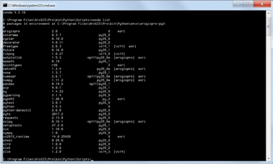
The first column shows the package name, the second the version of the package. The third column provides clues on how the package was installed. You will see that for some of the packages installed, Esri is listed, showing they are related to the Esri installation. The list option of conda is useful, not only to find out if the package you need is already installed but also to confirm that you have the appropriate version.
Conda has the functionality to create different environments. Think of an environment as a sandbox – you can set up the environment with a specific Python version and different packages. That allows you to work in environments with different packages and Python versions without affecting other applications. The default environment used by conda is called base environment. We do not need to create a new environment, but, should you need to, the process is simple – here is an example:
conda create -n gisenv python=3.6 arcpy numpy
the –n flag is followed by the name of the environment (in this case gisenv), then you would choose the Python version which matches the one you already have installed (3.5, 3.6 etc.) and follow that up with a list of packages you want to add to it. If you later find out you need other packages to be added, you could use the install option of conda, for example:
conda install –n gisenv matplotlib
To activate an environment, you would run:
activate gisenv
And to deactivate an environment, simply:
deactivate
There are other options you can use with environments – you can clone them and delete them, for example. A great resource for the different options is Conda's Managing Environments page.
2.8.3.1 Optional complementary materials: Installing Conda Build Package
Important note: While knowing how to create packages from your Python code to disseminate it is an important skill for a Python programmer, the procedure described in this section and section 2.8.3.2 is a bit complex and error-prone due to system and installation differences. It is also not required to have performed these steps successfully yourself to finish the lesson and the rest of the course. Therefore, this section is provided for interest only. We recommend that you just read through it or skip over it completely and you can then loop back to it at the end of the lesson if you have free time or after the end of the class. If you decide to go through the steps yourself and find yourself stuck with some errors, please feel free to ask about them on the course forums but don't let such issues keep you from reading through the rest of the section and finishing the lesson.
Before we can create a conda package of our own we do need to install the conda-build package. We will use conda to install the conda Build package, just as you did with the PyQT5 package.
Use the Python Command Prompt and type in:
conda install conda-build
What we are doing is running conda with the install option, and asking it to install the conda-build package. A search and analysis will be performed by conda to find the package, determine its dependencies and you will be informed of all the packages that will be installed. Type in y to allow the install to proceed, and you will get progress messages for the installation of conda-build and all packages it is dependent on.
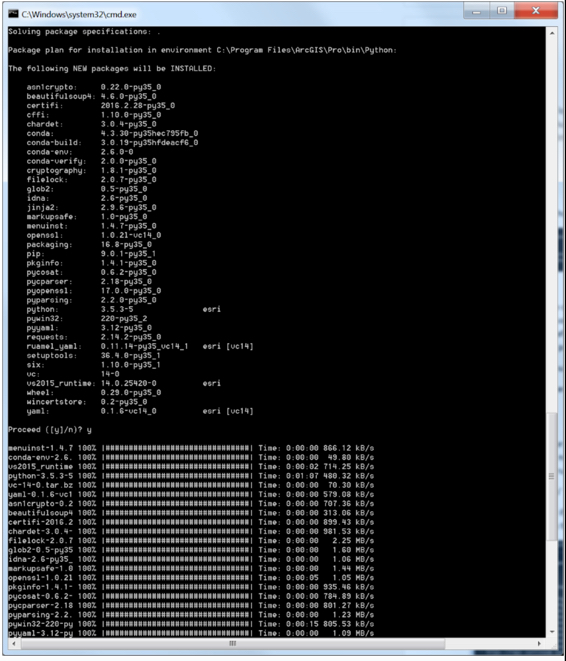
You could install other packages as well in a similar fashion (just as with pip), by changing the name conda-build to the appropriate package name. In order to know if a package you are looking for is available to be installed from conda, you can run conda with a search option, for example:
conda search pandas
The output will show if the package is available, and if so from which channels. Channels are different repositories that have been set up by users and organizations.
2.8.3.2 Optional complementary materials: Packaging Your Code with Conda
Important note: As the previous section, this section is provided for interest only. We recommend that you just read through it or skip over it completely and you can then loop back to it at the end of the lesson if you have free time or after the end of the class. If you decide to go through the steps yourself and find yourself stuck with some errors, please feel free to ask about them on the course forums but don't let such issues keep you from reading through the rest of the section and finishing the lesson.
Now that we know conda is installed and working, we will proceed to building your first conda package. Before we begin create a copy of your pip folder and rename it to conda. Delete the "dist" and "locationsfromwebservices.egg-info" folders. Creating a conda package will involve the following steps:
- Creating a meta.yaml file
- Creating a LICENSE file
- Creating a build.sh and bld.bat files
- Creating a setup.py file (we already created it while building the pip package)
- Building the project using conda-build
- Creating an account on Anaconda Cloud
- Uploading the project to Anaconda Cloud
We will walk through all these steps and create the necessary files and folders, just as we did for pip. For reference, as you are reading on, your final package folder and file structure should look like this for conda:
<yourinitialsdate>locationsfromwebservices
  ├── bld.bat
  ├── build.sh
  ├── LICENSE
  ├── meta.yaml
  ├── setup.py
  └── <yourinitialsdate>locationsfromwebservices
     ├── __init__.py
     ├── core_function.py
     ├── gui_main.py
     ├── gui_main.ui
     ├── gui_newshapefile.py
     ├── gui_newshapefile.ui
     └── main.py
The next step is to create a file named meta.yaml in the original (outer) <yourinitialsdate>locationsfromwebservices folder. You can create the file in any text editor. Make sure the name and extension match exactly. Type in the following into the file. Some of the elements will be left empty, but it is a good idea to use this template, to make sure all the elements you need are there:
package:
  name: <yourinitialsdate>locationsfromwebservicescomplete
  version: "1.0"

source:
  path: ./

requirements:
  build:
    - python
    - setuptools

  run:
    - python
    - pyqt

about:
  home: https://www.e-education.psu.edu/geog489/node/1867/
  license: BSD
  license_file: LICENSE
The package section of the file simply contains the package name and the version. The name can only contain lowercase letters and dashes.
The source sections point to the source of the data. In this case, we are pointing to the source on the local drive, but the source could be git or a compressed (.zip or .tar file), along with a few other options.
The requirements specify what tools are necessary to build the package, and the run section specifies what packages are necessary for running the package. Since we made the arcpy an optional part of the project we will not include it under the requirements. Setuptools is a package that helps with building Python projects. Please note that in conda the pyqt5 package is just called pyqt.
The about section provides more information about the package, such as the website it may be found on and license specification.
We set the license to BSD, which is a very permissive license type. Other licenses you may want to consider are GPL (General Public License) and LGPL (Lesser General Public License). A summary of these open source license types and a few others can be found at: choosealicense.com. It is a good idea to include a license with your package distribution. The name of the license file is specified in the about – license_file section, and it is typically named just license. You can download a sample license file here to be included with your distribution, or you can use the Binpress license generator and specify your own terms. Place the LICENSE file in the outer <yourinitialsdate>locationsfromwebservices folder where the meta.yaml file is located.
The version of the meta.yaml file we created is rather simple. There are other options you can set if necessary. Find the complete guide here.
Now we also need to create two build script files – build.sh and bld.bat. The .bat file works in the Windows environment, but, if the project is built on a Linux or a macOS environment (unlikely for arcpy type projects), we need the build.sh file as well.
Type in the following content into the bld.bat file:
"%PYTHON%" setup.py install
if errorlevel 1 exit 1
Here is the content for the build.sh file:
$PYTHON setup.py install
As you may have gathered from the batch files we created, the setup.py file is required by conda. Since we created it in setting up the pip package we do not need to recreate it here – just copy it from its location in your pip folder to the <yourinitialsdate>locationsfromwebservices folder within your conda folder.
Copy the LICENSE file into the <yourinitialsdate>locationsfromwebservices folder as well.
Now that we have the package set up, we will use the Python Command Prompt to build the package. Make sure you are in the folder that contains the outer <yourinitialsdate>locationsfromwebservices and run the following command:
conda-build <yourinitialsdate>locationsfromwebservices
After a long process and verbose output, towards the end you should see a line that gives you the command to upload your package to anaconda. More on this later. For now, just look at this output and note where the compressed tar.bz2 archive with your package has been created:
# If you want to upload package(s) to anaconda.org later, type:

anaconda upload c:\Users\<user name>\AppData\Local\ESRI\conda\envs\arcgispro-py3-clone\conda-bld\win-64\<yourinitialsdate>locationsfromwebservicescomplete-1.0-py35hc17e43c_0.tar.bz2
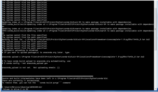
If you were watching the conda-build output very closely you might have seen a couple of errors displaying "The system cannot find the path specified" for some Visual Studio tools – that is okay and you do not need to be concerned by those.
That brings us to the next section of the lesson where we discuss Anaconda. Leave the Python Command Prompt window open, as we will be using it shortly to upload the package to the Anaconda Cloud.
2.8.3.3 Anaconda
Anaconda is a Python distribution that includes the most popular data science package and conda in its distribution. Anaconda makes it easy to create a Python setup conducive to data analytics that also facilitates package management (updates, installs), packaging projects, managing environments and sharing packages. It is build on top of conda but provides a graphical interface for managing Python environments and packages. Figure 40 obtained from the Anaconda website shows the Anaconda components.
If you investigate further you will learn that the conda portion of Anaconda contains a repository of packages maintained by Anaconda (Anaconda Repository), but also the Anaconda Cloud, which users and organizations can contribute to. If we were to upload the package created in the previous optional section with the command conda presented to us, it would be uploaded to the Anaconda Cloud.
We will use Anaconda in Lesson 3 to work in a fresh Python environment outside of the ArcGIS Pro installation. You should therefore perform the steps in this section to install Anaconda on your computer. Setting up a user account for Anaconda Cloud will be described in the following optional section. You won't need this unless you want try uploading the conda package from the previous optional section to the cloud yourself.
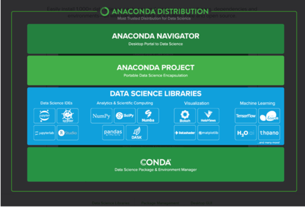
To download and install Anaconda you would normally go to anaconda.com, pick the Individual Edition option (or one of the other options if you prefer), and then click Download to get to the page where you can download the Anaconda installers (Figure 41; Anaconda frequently update their website design but you get the idea). However, we are here providing a direct link to download the Windows 64-bit installer to make sure we all are using the same version, one that we have tested the Lesson 3 content with: https://repo.anaconda.com/archive/Anaconda3-2021.05-Windows-x86_64.exe . Once downloaded double click on the .exe file to run the install. Use all the default install options. If asked, you can choose to skip installing Microsoft Visual Studio Code.
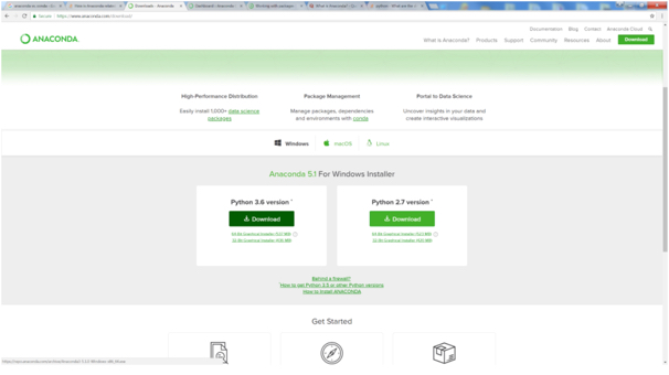
After the installation, Anaconda will be located in a folder called Anaconda3 of your user's home directory, so C:\Users\<user name>\Anaconda3 . This is the root environment (also called base environment) installed by Anaconda. If you create further environments or clone existing environments, these will be located in the envs subfolder of the Anaconda3 directory.
The easiest way to interact with Anaconda is via the Anaconda Navigator program that provides a graphical user interface for managing the installation, starting programs, etc. Just type the first letters into the Windows search and you should be able to find the program and run it (if not, it is located in the Scripts subfolder of the Anaconda3 directory).
Here is a quick overview of the Navigator interface: As shown in the image below, the Navigator has a vertical main menu on the left side of the window. We are only interested in the Home and Environments entries at the moment. The Home screen simply shows you a number of applications that are either installed and can be launched in your currently active Python environment or that you may want to install. You can switch to a different environment using the dropdown menu box at the top. In the image below, the currently active environment is the root environment installed by Anaconda.

If you now switch to the Environments screen, you will see that it has two main sections: the one on the left is for managing Python environments and the one on the right is for managing packages in the currently active environment. Anaconda will also see potential environments located under C:\Users\<user name>\AppData\Local\ESRI\conda\envs, so, if that's the location where your ArcGIS Pro installation has stored its default Python environment, it should appear in the environments list as well.
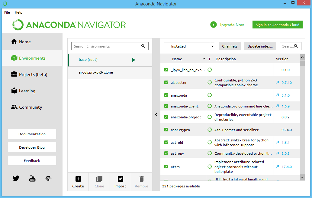
Clicking on a environment in the list will activate that environment and update the package manager view on the right accordingly. The buttons below the environment list can be used to easily create, clone or delete environments. The graphical package manager on the right is also relatively intuitive to use. At the top, you can (among other optios) select whether it should list the current, not installed, or all available packages. Selecting an uninstalled package by clicking the box on the very left of the entry will allow you to install that package. Packages for which newer versions are available are shown with a blue arrow next to the version number on the right. Clicking that arrow will allow you to update the package. Both the graphical environment manager and package manager are visual front-ends to conda. So whenever you perform some activity, like installing a package, the corresponding conda command will be executed in the background.
This was really just a very brief introduction to the main elements of the Anaconda Navigator and Anaconda in general. However, you will get the chance to further use it and learn more details in Lesson 3.
2.8.3.4 Optional complementary materials: Uploading Conda package to Anaconda Cloud
Important note: This section uses the conda package created in optional section 2.8.3.2. While knowing how to create packages from your Python code to disseminate it is an important skill for a Python programmer, it is not required to have performed the steps required in this section successfully yourself to finish the lesson and the rest of the course. Therefore, this section is provided for interest only. We recommend that you just read through it or skip over it completely and you can then loop back to it at the end of the lesson if you have free time or after the end of the class. If you decide to go through the steps yourself and find yourself stuck with some errors, please feel free to ask about them on the course forums but don't let such issues keep you from reading through the rest of the section and finishing the lesson.
After the installation, the next step to publishing our conda package from Section 2.8.3.2 is creating a user account. In order to obtain one, you need to go to anaconda.org and use the dialog on the right side of the screen to create an account.

Finally, we are ready to upload our package to Anaconda. In the Command Prompt window, run the following command to log into the Anaconda Cloud (note that the path might be one of the following two options depending on where Anaconda is installed):
c:\Users\YourUserName\Anaconda3\Scripts\anaconda login
or
c:\programdata\Anaconda3\Scripts\anaconda login
You will be asked to provide your user credentials and will be greeted with a message that confirms that your login was successful.
The next step is to upload your package – run the following command (remembering to use the path to where Anaconda was installed), but replace the tar.bz2 file with the file name conda provided you at the completion of the package build. If you are using an older version of Pro, you will also have to replace the first part of the path to the .tar.bz2 file with "c:\Program Files\ArcGIS\Pro\bin\Python\envs\arcgispro-py3\conda-bld\win-64\".
c:\Users\YourUserName\Anaconda3\Scripts\anaconda upload "c:\Users\<user name>\AppData\Local\ESRI\conda\envs\arcgispro-py3-clone\conda-bld\win-64\<yourinitialsdate>locationsfromwebservicescomplete-1.0-py35hc17e43c_0.tar.bz2"
You will receive messages that keep you updated on the upload status, and then you will be notified that the upload is complete. Log into the Anaconda Cloud and look at your Dashboard (Figure 43) – the package is now listed, and located in your own Anaconda Cloud Channel. If you click on the package name you will receive information on how it can be installed with conda.
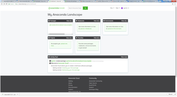
2.8.4 Package Distribution Recommendation - Why Conda?
If you worked or read through the exercises we worked through for packaging our application in the optional parts of this section, you might have gotten the impression that pip is easier to use than conda, and, since they both facilitate software packaging and distribution, why bother packaging your applications with conda? Here are a number of reasons:
- Conda has a built-in virtual environment functionality
- Conda further aids in package installs as it not only checks for dependencies but installs any dependent packages
- Conda is closely bound with Anaconda and Anaconda Cloud, which is set up to use different channels, providing a finer-grained package organization. For example, if you are interested in packages ESRI has published, you can go to the company’s channel - https://anaconda.org/esri.
- While pip can only be used with Python, conda can be used with other languages as well – so if you decided to develop something with R, conda can work with it too.
If you are interested in a more detailed comparison of the two tools, a great article to reference is Conda Myths and Misconceptions.
2.9 Lesson 2 Practice Exercises
After this excursion into the realm of package management and package managers, let's come back to the previous topics covered in this lesson (list comprehension, web access, GUI development) and wrap up the lesson with a few practice exercises. These are meant to give you the opportunity to test how well you have understood the main concepts from this lesson and as a preparation for the homework assignment in which you are supposed to develop a small standalone and GUI-based program for a relatively simple GIS workflow using arcpy. Even if you don't manage to implement perfect solutions for all three exercises yourself, thinking about them and then carefully studying the provided solutions will be helpful, in particular since reading and understanding other people's code is an important skill and one of the main ways to become a better programmer. The solutions to the three practice exercises can be found in the following subsections.
Practice Exercise 1: List Comprehension
You have a list that contains dictionaries describing spatial features, e.g. obtained from some web service. Each dictionary stores the id, latitude, and longitude of the feature, all as strings, under the respective keys "id", "lat", and "lon":
features = [ { "id": "A", "lat": "23.32", "lon": "-54.22" },
             { "id": "B", "lat": "24.39", "lon": "53.11" },
             { "id": "C", "lat": "27.98", "lon": "-54.01" } ]
We want to convert this list into a list of 3-tuples instead using a list comprehension (Section 2.2). The first element of each tuple should be the id but with the fixed string "Feature " as prefix (e.g. "Feature A"). The other two elements should be the lat and lon coordinates but as floats not as strings. Here is an example of the kind of tuple we are looking for, namely the one for the first feature from the list above: ('Feature A', 23.32, -54.22). Moreover, only features with a longitude coordinate < 0 should appear in the new list. How would you achieve this task with a single list comprehension?
Practice Exercise 2: Requests and BeautifulSoup4
We want to write a script to extract the text from the three text paragraphs from section 1.7.2 on profiling without the heading and following list of subsections. Write a script that does that using the requests module to load the html code and BeautifulSoup4 to extract the text (Section 2.3).
Finally, use a list comprehension (Section 2.2) to create a list that contains the number of characters for each word in the three paragraphs. The output should start like this:
[2, 4, 12, 4, 4, 4, 6, 4, 9, 2, 11… ]
Hint 1If you use Inspect in your browser, you will see that the text is the content of a <div> element within another <div> element within an <article> element with a unique id attribute (“node-book-2269”). This should help you write a call of the soup.select(…) method to get the <div> element you are interested in. An <article> element with this particular id would be written as “article#node-book-2269” in the string given to soup.select(…).
Hint 2:Remember that you can get the plain text content of an element you get from BeautifulSoup from its .text property (as in the www.timeanddate.com example in Section 2.3).
Hint 3It’s ok not to care about punctuation marks, etc. in this exercise and simply use the string method split() to split the text into words at any whitespace character. The number of characters in a string can be computed with the Python function len(...).
Practice Exercise 3: GUI Development
The goal of this exercise is to practice creating GUIs a little bit more. Your task is to implement a rudimentary calculator application for just addition and subtraction that should look like the image below:
The buttons 0… 9 are for entering the digits into the line input field at the top. The buttons + and - are for selecting the next mathematical operation and performing the previously selected one. The = button is for performing the previously selected operation and printing out the result, and the “Clear” button is for resetting everything and setting the content of the central line edit widget to 0. At the top of the calculator we have a combo box that will list all intermediate results and, on selection of one of the entries, will place that number in the line edit widget to realize a simple memory function.
Here is what you will have to do:
- Create the GUI for the calculator with QT Designer using the “Widget” template. This calculator app is very simple so we will use QWidget for the main window, not QMainWindow. Make sure you use intuitive object names for the child widgets you add to the form. (See Sections 2.6.2 and 2.7.2)
- Compile the .ui file created in QT Designer into a .py file (Sections 2.6.2 and 2.7.2).
- Set up a main script file for this project and put in the code to start the application and set up the main QWidget with the help of the .py file created in step 2 (Sections 2.6.1 and 2.7.3).
Hint 1: To produce the layout shown in the figure above, the horizontal and vertical size policies for the 10 digit buttons have been set to “Expanding” in QT Designer to make them fill up the available space in both dimensions. Furthermore, the font size for the line edit widget has been increased to 20 and the horizontal alignment has been set to “AlignRight”.
This is the main part we want you to practice with this exercise. You should now be able to run the program and have the GUI show up as in the image above but without anything happening when you click the buttons. If you want, you can continue and actually implement the functionality of the calculator yourself following the steps below, or just look at the solution code showing you how this can be done.
- Set up three global variables: intermediateResult for storing the most recent intermediate result (initialized to zero); lastOperation for storing the last mathematical operation picked (initialized to None); and numberEntered for keeping track of whether or not there have already been digits entered for a new number after the last time the +, -, = or Clear buttons have been pressed (initialized to False).
- Implement the event handler functions for the buttons 0 … 9 and connect them to the corresponding signals. When one of these buttons is pressed, the digit should either be appended to the text in the line edit widget or, if its content is “0” or numberEntered is still False, replace its content. Since what needs to happen here is the same for all the buttons, just using different numbers, it is highly recommended that you define an auxiliary function that takes the number as a parameter and is called from the different event handler functions for the buttons.
- Implement an auxiliary function that takes care of the evaluation of the previously picked operation when, e.g., the = button is clicked. If lastOperation contains an operation (so is not None), a new intermediate result needs to be calculated by applying this operation to the current intermediate result and the number in the line edit widget. The new result should appear in the line edit widget. If lastOperation is None, then intermediateResult needs to be set to the current text content of the line input widget. Create the event handler function for the = button and connect it to this auxiliary function.
- Implement and connect the event handler functions for the buttons + and - . These need to call the auxiliary function from the previous step and then set lastOperation to a string value representing the new operation that was just picked, either "+" or "-".
- Implement and connect the event handler for the “Clear” button. Clicking it means that the global variables need be re-initialized as in step 4 and the text content of the line edit widget needs to be set back to “0”.
- Implement the combo box functionality: whenever a calculation is performed by the auxiliary function from step 6, you now also need to add the result to the item list of the memory combo box. Furthermore, you need to implement and connect the event handler for when a different value from the combo box is picked and make this the new text content of the line edit field. The signal of the combo box you need to connect to for this is called “activated”.
2.9.1 Lesson 2 Practice Exercise 1 Solution
features = [ { "id": "A", "lat": "23.32", "lon": "-54.22" },
             { "id": "B", "lat": "24.39", "lon": "53.11" },
             { "id": "C", "lat": "27.98", "lon": "-54.01" } ]

featuresAsTuples = [ ("Feature " + feat['id'], float(feat['lat']), float(feat['lon']) ) for feat in features if float(feat['lon']) < 0 ]

print(featuresAsTuples)
Let's look at the components of the list comprehension starting with the middle part:
for feat in features
This means we will be going through the list features using a variable feat that will be assigned one of the dictionaries from the features list. This also means that both the if-condition on the right and the expression for the 3-tuples on the left need to be based on this variable feat.
if float(feat['lon']) < 0
Here we implement the condition that we only want 3-tuples in the new list for dictionaries that contain a lon value that is < 0.
("Feature " + feat['id'], float(feat['lat']), float(feat['lon']) )
Finally, this is the part where we construct the 3-tuples to be placed in the new list based on the dictionaries contained in variable feat. It should be clear that this is an expression for a 3-tuple with different expressions using the values stored in the dictionary in variable feat to derive the three elements of the tuple. The output produced by this code will be:
Output:

[('Feature A', 23.32, -54.22), ('Feature C', 27.98, -54.01)]
2.9.2 Lesson 2 Practice Exercise 2 Solution
import requests
from bs4 import BeautifulSoup

url = 'https://www.e-education.psu.edu/geog489/node/2269'

response = requests.get(url)
soup = BeautifulSoup(response.text, 'html.parser')

divElement = soup.select('article#node-book-2269 > div > div')[0]

wordLengths = [ len(word) for word in divElement.text.split() ]
print(wordLengths)
After loading the html page and creating the BeautifulSoup structure for it as in the examples you already saw in this lesson, the select(…) method is used in line 9 to get the <div> elements within the <div> element within the <article> element with the special id we are looking for. Since we know there will only be one such element, we can use the index [0] to get that element from the list and store it in variable divElement.
With divElement.text.split() we create a list of all the words in the text and then use this inside the list comprehension in line 11 where we convert the word list into a list of word lengths by applying the len(…) function to each word.
2.9.3 Lesson 2 Practice Exercise 3 Solution
The image below shows the hierarchy of widgets created in QT Designer and the names chosen. You can also download the .ui file and the compiled .py version here and open the .ui file in QT Designer to compare it to your own version. Note that we are using a vertical layout as the main layout, a horizontal layout within that layout for the +, -, =, and Clear button, and a grid layout within the vertical layout for the digit buttons.
The following code can be used to set up the GUI and run the application but without yet implementing the actual calculator functionality. You can run the code and main window with the GUI you created will show up.
import sys

from PyQt5.QtWidgets import QApplication, QWidget

import calculator_gui

# create application and gui

app = QApplication(sys.argv)

mainWindow = QWidget()        # create an instance of QWidget for the main window
ui = calculator_gui.Ui_Form() # create an instance of the GUI class from calculator_gui.py
ui.setupUi(mainWindow)        # create the GUI for the main window

# run app

mainWindow.show()
sys.exit(app.exec_())
The main .py file for the full calculator can be downloaded here. Function digitClicked(…) is the auxiliary function from step 5, called by the ten event handler functions digitPBClicked(…) defined later in the code. Function evaluateResult() is the auxiliary function from step 6. Function operatorClicked(…) is called from the two event handler functions plusPBClicked() and minusPBClicked(), just with different strings representing the mathematical operation. There are plenty of comments in the code, so it should be possible to follow along and understand what is happening rather easily.
2.10 Lesson 2 Assignment
In this lesson's homework assignment you are going to implement your own GUI-based Python program with PyQt5. We won't provide a template for the GUI this time, so you will have to design it yourself from scratch and put it together in QT Designer. However, we will provide a list of required GUI elements that will allow the user to provide the needed input for the program. The program will use arcpy but it is intended to be a standalone program, so it's not supposed to be run as a script tool inside ArcGIS, and that's why it needs its own GUI. The program will realize a simple workflow for extracting features from a shapefile on disk based on selection by attribute and selection by location. If you took Geog485 along time ago, you will notice that this is similar to what you did there in lesson 3 and you will also already be familiar with the data we will be using. If you took Geog485 more recently and did the assignment with NHL hockey players, it's still a similar approach using multiple selection operations but with different data. Even if it's unfamiliar, don't worry, we are intentionally keeping the feature extraction task simple and providing some sample code that you can use for this so that you can focus on the GUI development aspects.
Data
Please download the zip file assignment2data.zip with the data you will need for this homework project. Extract the data to a new folder and check out the two shapefiles that are contained in the zip file, countries.shp and OSMpoints.shp, in ArcGIS Pro. In particular, have a look at the attribute tables of the two files:
- countries. shp - This shapefile contains polygons for the countries of Central America and will be used for the selection by location part of the project, namely to extract only features that are inside one of the countries. The field you will mainly be working with is the 'NAME' field containing the names of the countries. To test your program, you will mainly use 'El Salvador' for the country you are interested in because the data from the other shapefile is limited to an area in and around El Salvador.
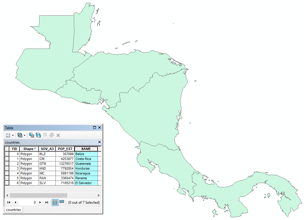
- OSMpoints.shp - This is a point shapefile with Points of Interests (POIs) exported from OpenStreetMap. The file is a bit messy, has quite a few attribute fields, and combines all kinds of POIs. In this assignment, we will be working with the 'shop' field that, if the feature is some kind of shop, specifies what kind of shop it is, e.g. supermarket, convenience, bakery. Our program will either extract all shops in a target country or only shops of one particular type.
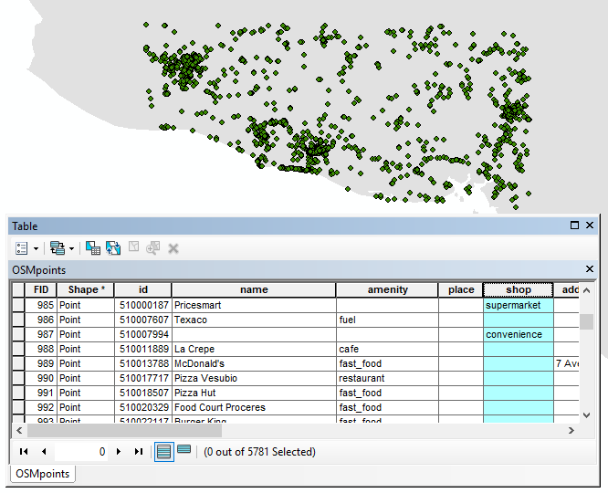
The feature extraction task
Your program will provide the GUI that allows the user
- to select the two input files (country file and POI file),
- to provide the name of the target country,
- to specifiy the name of the output shapefile that will be produced with the extracted shop features,
- and to indicate whether all shops or only shops of a particular type should be extracted (and if so, which type).
Then, when the user clicks a button to start the feature extraction, your code will have to select those point features from the POI file that are at the same time (a) located inside the target country and (b) are shops (meaning the 'shop' field is not null and not an empty string) if the user wants all shops. If the user indicated that s/he is only interested in shops of a particular type, only shops of that specified type should be selected (meaning the 'shop' field needs to contain exactly that type for a POI to be selected). After realizing these selections, the selected features satisfying both criteria should be written to a new shapefile with the user-provided output file name.
Hopefully it is clear that this feature extraction can be realized with a combination of the arcpy functions MakeFeatureLayer_management(...), SelectLayerByLocation_management(....), CopyFeatures_management(...) and Delete_management(...). If not, you may want to briefly (re)read the parts of Lesson 3 of Geog485 that talk about these functions or the appropriate sections of the arcpy help. The field names 'NAME' and 'shop' can be hard-coded in your script but only once in variables defined at the beginning that are then used in the rest of the code (so that your code is easily modifiable in-line with good programming practices). As we mentioned at the beginning, we want you to focus on GUI code, so we are, below, providing some basic sample code for performing the extraction task that you can adopt. Of course, you are free to challenge yourself and ignore this code and develop a solution for this extraction part yourself.
# This code uses the following variables:
# polygonFile: input polygon file (e.g. file with countries)
# polygonField: name of field of the input polygon file to query on (e.g. 'NAME')
# polygonValue: value to query polygonField for (e.g. 'El Salvador')
# pointFile: input point file (e.g. file with points of interest)
# pointField: name of field of the input point file to query on (e.g. 'shop')
# pointValue: value to query pointField for (e.g. 'supermarket'); if this variable has the value None, all features with something in pointField will be included
# outputFile: name of the output shapefile to produce

# select target polygon from polygon file
polygonQuery = '"{0}" = \'{1}\''.format(polygonField, polygonValue)          # query string
arcpy.MakeFeatureLayer_management(polygonFile,"polygonLayer", polygonQuery)  # produce layer based on query string

# select target points from point file
if pointValue:   # not None, so the query string needs to use pointValue
    pointQuery = '"{0}" = \'{1}\''.format(pointField, pointValue)
else:            # pointValue is None, so the query string aks for entries that are not NULL and not the empty string
    pointQuery = '"{0}" IS NOT NULL AND "{0}" <> \'\''.format(pointField)
arcpy.MakeFeatureLayer_management(pointFile,"pointLayer", pointQuery)        # produce layer based on query string

# select only points of interest in point layer that are within the target polygon
arcpy.SelectLayerByLocation_management("pointLayer", "WITHIN", "polygonLayer")

# write selection to output file
arcpy.CopyFeatures_management("pointLayer", outputFile)

# clean up layers
arcpy.Delete_management("polygonLayer")
arcpy.Delete_management("pointLayer")
You are expected to place the code that performs this feature extraction task in its own function and its own .py file that is completely independent of the rest of the code in the same way as we did in the lesson's walkthrough with the functions defined in the core_functions.py module. This extraction function needs to have parameters for all input values needed to perform the feature extraction task and produce the output shapefile.
It is definitely not a bad idea to start with producing the feature extraction function/module first (adopting the code from above) and in the code that calls the function use hard-coded input variables for all input values for thoroughly testing that function. Then only start with designing and implementing the GUI, once the feature extraction function is working correctly. As mentioned above, the provided test data mainly contains POI features for El Salvador but you can also test it with one of the adjacent countries that contain some of the point features.
The GUI
As already explained, the main focus of this project will be on designing the GUI for this program, putting it together in QT Designer, and then creating the GUI for the main project code and wiring everything up so that the input values are taken from the corresponding input widgets in the GUI when the button to run the feature extraction is clicked, and so on. These steps can be approached in the same way as we did in the lesson's walkthrough and the project will also have a similar structure.
Designing the GUI will require some creativity and you are free to decide how the different GUI elements should be arranged in your GUI. However, you should make sure that the elements are laid out nicely and the overall GUI is visually appealing. Even though this is just a "toy" project to practice these things, you should try to make your GUI look as professional as possible, e.g. don't forget to give your main window a suitable title, use labels to explain what certain widgets are for, group related widgets together, make adequate use of file dialog boxes and message boxes, etc.
Below is a list of elements that your GUI needs to provide and other requirements we have for your GUI and code. Please don't take the order in which the elements are listed here as the order in which they are supposed to appear in your GUI.
- The GUI should contain a button to start the feature extraction for the input values provided via the other widgets.
- The GUI should contain an input widget for the name of the country shapefile. There should be a corresponding button to open an "Open file" dialog box to pick the country shapefile (similar to how this was done in the Locations From Web Services tool; see, for instance, the code of the selectShapefile() function in Section 2.7.3.5).
- The GUI should contain an input widget for the name of the POI point shapefile. There should be a corresponding button to open an "Open file" dialog box to pick the point shapefile (similar to how this was done in the Locations From Web Services tool; see, for instance, the code of the selectShapefile() function in Section 2.7.3.5).
- The GUI should contain an input widget for the name of the output shapefile. There should be a corresponding button to open a "Save file" dialog box to pick the output shapefile name (similar to how this was done in the Locations From Web Services tool; see, for instance, the code of the selectNewShapefile() function in Section 2.7.3.5).).
- The GUI should contain an input widget for entering the name of the target country (you are not required to create a list of available country names for this; a widget that allows the user to type in the name is ok for this, or a hardcoded list providing it is drawn from a variable defined at the top of the code).
- The GUI should contain an input widget that lets the user indicate whether all shops or only shops of a particular type should be extracted with a single mouse button click. (This should be a separate widget from the following one for choosing a specific shop type if the user picks the "shops of a particular type" option!)
- The GUI should contain an input widget that allows the user to pick a shop type from a given list of predefined types. You can use the following set of predefined shop types for this: [ 'supermarket', 'convenience', 'clothes', 'bakery' ]. Selecting one of the predefined types should be done by clicking, not by letting the user type in the name of the shop type.
- Your program should capture errors and use message boxes to inform the user about errors or when the feature extraction has been performed successfully (see again how this is handled in the walkthrough code).
- The GUI independent code to perform the actual feature extraction (see previous section) should be located in its own module which is imported by the main module of your project.
- The usual requirements regarding code quality and use of comments apply; please make sure that you use intuitive names for the widgets that you are referring to from the main project code.
Successful completion of the above requirements and the write-up discussed below is sufficient to earn 90% of the credit on this project. The remaining 10% is reserved for "over and above" efforts which could include, but are not limited to, the following (implementing just the first two items is not sufficient for the full 10 points):
- Providing helpful tool tip information for all main GUI elements.
- Adding input widgets for the field names to replace the hard-coded values 'NAME' and 'shop'
- Incorporating additional widgets that increase the flexibility of the tool (e.g. you could add support for providing a buffer radius that is applied to the country before doing the selection by location, or an optional projection operation to be applied to the output file using one of several predefined spatial reference system names the user can choose from).
- Populating the list of shop types to choose from automatically with all unique values appearing in the shop column of the selected POI input file whenever the name of the POI input file is changed.
- Replacing the widget that allows the user to type in the name of the target country by a widget that lists the names of all country names in the country input file and allows the user to pick one (or even several) of them.
All files making up your project should be included in your submission for this assignment including the .ui file created with QT Designer. Please also include a screenshot showing the GUI of your program while the program is being executed. If as part of your "over and above" efforts you are making changes that result in the project not satisfying the original conditions from the list above anymore, please include both your original solution and the modified version in your submission as two separate folders.
Write-up
Produce a 400 word write-up of what you have learned during this exercise; reflect on and briefly discuss the decisions you made when you designed the GUI for this project. Please also briefly mention what you did for "over and above" points in the write-up.
Deliverables
Submit a single .zip file to the Programming Assignment drop box; the zip file should contain:
- all the code and .ui files for your project
- a screenshot showing the GUI of the running project
- your 400 word write-up
Lesson 3 Python Geo and Data Science Packages & Jupyter Notebooks
3.1 Overview and Checklist
This lesson is two weeks in length. We will introduce a few more Python programming concepts and then focus on conducting (spatial) data science projects in Python with the help of Jupyter Notebooks. In the process, you will get to know quite a few more useful Python packages and 3rd-party APIs including pandas, GDAL/OGR, and the Esri ArcGIS for Python API.
Please refer to the Calendar for specific time frames and due dates. To finish this lesson, you must complete the activities listed below. You may find it useful to print this page first so that you can follow along with the directions.
| Step | Activity | Access/Directions |
|---|---|---|
| 1 | Engage with Lesson 3 Content | Begin with 3.2 Installing the required packages for this lesson |
| 3 |
Programming Assignment and Reflection |
Submit your code for the programming assignment and 400 words write-up with reflections |
| 4 | Quiz 3 | Complete the Lesson 3 Quiz |
| 5 | Questions/Comments | Remember to visit the Lesson 2 Discussion Forum to post/answer any questions or comments pertaining to Lesson 3 |
3.2 Installing the required packages for this lesson
This lesson will require quite a few different Python packages. We will take care of this task right away so that you then won't have to stop for installations when working through the lesson content. We will use our Anaconda installation from Lesson 2 and create a fresh Python environment within it. In principle, you could perform all the installations with a number of conda installation commands from the command line. However, there are a lot of dependencies between the packages and it is relatively easy to run into some conflicts that are difficult to resolve. Therefore, we instead provide a YAML .yml file that lists all the packages we want in the environment with the exact version and build numbers we need. We create the new environment by importing this .yml file using conda in the command line interface ("Anaconda Prompt"). For reference, we also provide the conda commands used to create this environment at the end of this section. Also important to note is that one of the packages we will be working with in this lesson is the ESRI ArcGIS for Python API, which will require a special approach to authenticate with your PSU login. You will already see this approach further down below and it will then be explained further in Section 3.10.
Creating the Anaconda Python environment
Please follow the steps below and if you get issues we've got an alternative approach below.
If you're having issues you'll notice adjacent links to download a YAML file and to use that everywhere below you see "37" please replace it with "38" even if you've got v3.9 - there's no current technical difference between v3.8 & v3.9 for this lesson and in reality the ac37 should work no matter which version you're using. That might sound a little confusing but you should be ok with the AC37 file but just in case we've got some fallbacks. If you have trouble creating the environment from the YAML file there's specific instructions below.
1) Download the .zip file containing the .yml file from this link: ac37_Fall2023.zip (AC38_SP24.zip only if required), then extract the file .yml it contains. You may want to have a quick look at the content of this text file to see how, among other things, it lists the names of all packages for this environment with version and build numbers. Using a YAML file greatly speeds up the creation of the environment as the files are downloaded and dependencies don't need to be resolved on the fly by conda.
2) Open the program called "Anaconda Prompt" which is part of the Anaconda installation from Lesson 2.
3) Make sure you have at least 5GB space on your C: drive (the environment will require around 3.5-4GB). Then type in and run the following conda command to create a new environment called AC37 (for Anaconda Python 3.7 or AC38 for Python 3.8) from the downloaded .yml file. You will have to replace the ... to match the name of the .yml file and maybe also adapt the path to the .yml file depending on where you have it stored on your harddisk.
conda env create --name AC37 -f "C:\489\ac37_....yml"
Conda will now create the environment called AC37 (AC38 if you're using that other file above for Python v3.8) according to the package list in the YAML file. This can take quite a lot of time; in particular, it will just say "Solving environment" for quite a while before anything starts to happen. If you want, you can work through the next few sections of the lesson while the installation is running. The first section that will require this new Python environment is Section 3.6. Everything before that can still be done in the ArcGIS environment you used for the first two lessons. When the installation is done, the AC37 (AC38 for Python v3.8) environment will show up in the environments list in the Anaconda Navigator and will be located at C:\Users\<user name>\Anaconda3\envs\AC37 .
4) Let's now do a quick test to see if the new environment works as intended. In the Anaconda Prompt, activate the new environment with the following command (you'll need to activate your environment every time you want to use it):
activate AC37
Then type in python and in Python run the following commands; all the modules should import without any error messages:
import bs4
import pandas
import cartopy
import matplotlib
from osgeo import gdal
import geopandas
import rpy2
import shapely
import arcgis
from arcgis.gis import GIS
As a last step, let's test connecting to ArcGIS Online with the ArcGIS for Python API mentioned at the beginning. Run the following Python command:
gis = GIS('https://pennstate.maps.arcgis.com', client_id='lDSJ3yfux2gkFBYc')
Now a browser window should open up where you have to authenticate with your PSU login credentials (unless you are already logged in to Penn State). After authenticating successfully, you will get a window saying "OAuth2 Approval" and a box with a very long code at the bottom. In the Anaconda Prompt window, you will see a prompt saying "Enter code obtained on signing in using SAML:". Use CTRL+A and CTRL+C to copy the entire code, and then do a right-click with the mouse to paste the code into the Anaconda Prompt window. The code won't show up, so just continue by pressing Enter.
If you are having troubles with this step, Figure 3.18 in Section 3.10 illustrates the steps. You may get a short warning message (InsecureRequestWarning) but as long as you don't get a long error message, everything should be fine. You can test this by running this final command:
print(gis.users.me)
This should produce an output string that includes your pennstate ArcGIS Online user name, so e.g., <User username:xyz12_pennstate> . More details on this way of connecting with ArcGIS Online will be provided in Section 3.10.
If creating the environment from the .yml file did NOT work:
Creating the AC37 environment from scratch with Conda
As we wrote above, importing the .yml file with the complete package and version number list is probably the most reliable method to set up the Python environment for this lesson but there have been cases in the past where using this approach failed on some systems. Or maybe you are interested in the steps that were taken to create the environment from scratch. We therefore list the conda commands used from the Anaconda Prompt for reference below.
1) Create a new conda Python 3.7 environment called AC37 with some of the most critical packages:
conda create -n AC37 -c conda-forge -c esri python=3.7 nodejs arcgis=2 gdal=3 jupyter ipywidgets=7.6.0
2) As we did in Lesson 2, we activate the new environment using:
activate AC37
3) Then we add the remaining packages:
conda install -c conda-forge rpy2=3.4.1
conda install -c conda-forge r-raster=3.4_5
conda install -c conda-forge r-dismo=1.3_3
conda install -c conda-forge r-maptools
conda install -c conda-forge geopandas
conda install -c conda-forge cartopy
4) Once we have made sure that everything is working correctly in this new environment, we can export a YAML file similar to the one we have been using in the first part above using the command:
conda env export > AC37.yml
If creating the environment from the AC38.yml file did NOT work:
Creating the AC38 environment from scratch with Conda
As we wrote above, importing the .yml file with the complete package and version number list is probably the most reliable method to set up the Python environment for this lesson but there have been cases in the past where using this approach failed on some systems. Or maybe you are interested in the steps that were taken to create the environment from scratch. We therefore list the conda commands used from the Anaconda Prompt for reference below.
1) Create a new conda Python 3.8 environment called AC38 with some of the most critical packages (and you'll notice there's some additional package version numbers specified to handle inconsistencies in V3.8/V3.9):
conda create -n AC38 -c conda-forge -c esri python=3.8 nodejs arcgis=2 gdal=3 jupyter ipywidgets=7.6.0 requests=2.29.0 urllib3=1.26.18
2) As we did in Lesson 2, we activate the new environment using:
activate AC38
3) Then we add the remaining packages:
conda install -c conda-forge rpy2=3.4.1
conda install -c conda-forge r-raster=3.4_5
conda install -c conda-forge r-dismo=1.3_3
conda install -c conda-forge r-maptools
conda install -c conda-forge geopandas
conda install -c conda-forge cartopy  matplotlib=3.5.3 pillow=9.2.0 shapely=1.8.5 fiona=1.8.22
4) Once we have made sure that everything is working correctly in this new environment, we can export a YAML file similar to the one we have been using in the first part above using the command:
conda env export > AC38.yml
Potential issues
There is a small chance that the from osgeo import gdal will throw an error about DLLs not being found on the path which looks like the below:
During handling of the above exception, another exception occurred:
Traceback (most recent call last):

	  File "<stdin>", line 1, in <module>

	  File "C:\Users\jao160\anaconda3\envs\AC38_SP24\lib\site-packages\osgeo\__init__.py", line 46, in <module>

	    _gdal = swig_import_helper()

	  File "C:\Users\jao160\anaconda3\envs\AC38_SP24\lib\site-packages\osgeo\__init__.py", line 42, in swig_import_helper

	    raise ImportError(traceback_string + '\n' + msg)

	ImportError: Traceback (most recent call last):

	  File "C:\Users\jao160\anaconda3\envs\AC38_SP24\lib\site-packages\osgeo\__init__.py", line 30, in swig_import_helper

	    return importlib.import_module(mname)

	  File "C:\Users\jao160\anaconda3\envs\AC38_SP24\lib\importlib\__init__.py", line 127, in import_module

	    return _bootstrap._gcd_import(name[level:], package, level)

	  File "<frozen importlib._bootstrap>", line 1014, in _gcd_import

	  File "<frozen importlib._bootstrap>", line 991, in _find_and_load

	  File "<frozen importlib._bootstrap>", line 975, in _find_and_load_unlocked

	  File "<frozen importlib._bootstrap>", line 657, in _load_unlocked

	  File "<frozen importlib._bootstrap>", line 556, in module_from_spec

	  File "<frozen importlib._bootstrap_external>", line 1166, in create_module

	  File "<frozen importlib._bootstrap>", line 219, in _call_with_frames_removed

	ImportError: DLL load failed while importing _gdal: The specified module could not be found.
On Windows, with Python >= 3.8, DLLs are no longer imported from the PATH.

	If gdalXXX.dll is in the PATH, then set the USE_PATH_FOR_GDAL_PYTHON=YES environment variable

	to feed the PATH into os.add_dll_directory().
In the event this happens the fix is to (every time you want to import gdal you would need to do this):
import os

	os.environ["USE_PATH_FOR_GDAL_PYTHON"]="YES"

	from osgeo import gdal
It's possible the above fix doesn't work and the error is still thrown which will require checking the PATH environment variable in the Anaconda Prompt by typing "path" and checking that c:\osgeo42\bin or osgeo4w64\bin is in the list and if not adding it using set path=%PATH%;c:\osgeo4w\bin
3.3 Regular expressions
To start off Lesson 3, we want to talk about a situation that you regularly encounter in programming: Often you need to find a string or all strings that match a particular pattern among a given set of strings.
For instance, you may have a list of names of persons and need all names from that list whose last name starts with the letter ‘J’. Or, you want do something with all files in a folder whose names contain the sequence of numbers “154” and that have the file extension “.shp”. Or, you want to find all occurrences where the word “red” is followed by the word “green” with at most two words in between in a longer text.
Support for these kinds of matching tasks is available in most programming languages based on an approach for denoting string patterns that is called regular expressions.
A regular expression is a string in which certain characters like '.', '*', '(', ')', etc. and certain combinations of characters are given special meanings to represent other characters and sequences of other characters. Surely you have already seen the expression “*.txt” to stand for all files with arbitrary names but ending in “.txt”.
To give you another example before we approach this topic more systematically, the following regular expression “a.*b” in Python stands for all strings that start with the character ‘a’ followed by an arbitrary sequence of characters, followed by a ‘b’. The dot here represents all characters and the star stands for an arbitrary number of repetitions. Therefore, this pattern would, for instance, match the strings 'acb', 'acdb', 'acdbb', etc.
Regular expressions like these can be used in functions provided by the programming language that, for instance, compare the expression to another string and then determine whether that string matches the pattern from the regular expression or not. Using such a function and applying it to, for example, a list of person names or file names allows us to perform some task only with those items from the list that match the given pattern.
In Python, the package from the standard library that provides support for regular expressions together with the functions for working with regular expressions is simply called “re”. The function for comparing a regular expression to another string and telling us whether the string matches the expression is called match(...). Let’s create a small example to learn how to write regular expressions. In this example, we have a list of names in a variable called personList, and we loop through this list comparing each name to a regular expression given in variable pattern and print out the name if it matches the pattern.
import re

personList = [ 'Julia Smith', 'Francis Drake', 'Michael Mason',
                'Jennifer Johnson', 'John Williams', 'Susanne Walker',
                'Kermit the Frog', 'Dr. Melissa Franklin', 'Papa John',
                'Walter John Miller', 'Frank Michael Robertson', 'Richard Robertson',
                'Erik D. White', 'Vincent van Gogh', 'Dr. Dr. Matthew Malone',
                'Rebecca Clark' ]

pattern = "John"

for person in personList:
    if re.match(pattern, person):
        print(person)
Output:

John Williams
Before we try out different regular expressions with the code above, we want to mention that the part of the code following the name list is better written in the following way:
pattern = "John"

compiledRE = re.compile(pattern)

for person in personList:
    if compiledRE.match(person):
        print(person)
Whenever we call a function from the “re” module like match(…) and provide the regular expression as a parameter to that function, the function will do some preprocessing of the regular expression and compile it into some data structure that allows for matching strings to that pattern efficiently. If we want to match several strings to the same pattern, as we are doing with the for-loop here, it is more time efficient to explicitly perform this preprocessing and store the compiled pattern in a variable, and then invoke the match(…) method of that compiled pattern. In addition, explicitly compiling the pattern allows for providing additional parameters, e.g. when you want the matching to be done in a case-insensitive manner. In the code above, compiling the pattern happens in line 3 with the call of the re.compile(…) function and the compiled pattern is stored in variable compiledRE. Instead of the match(…) function, we now invoke the method match(…) of the compiled pattern object in variable person (line 6) that only needs one parameter, the string that should be matched to the pattern. Using this approach, the compilation of the pattern only happens once instead of once for each name from the list as in the first version.
One important thing to know about match(…) is that it always tries to match the pattern to the beginning of the given string but it allows for the string to contain additional characters after the entire pattern has been matched. That is the reason why when running the code above, the simple regular expression “John” matches “John Williams” but neither “Jennifer Johnson”, “Papa John”, nor “Walter John Miller”. You may wonder how you would then ever write a pattern that only matches strings that end in a certain sequence of characters. The answer is that Python's regular expressions use the special characters ^ and $ to represent the beginning or the end of a string and this allows us to deal with such situations as we will see a bit further below.
Now let’s have a look at the different special characters and some examples using them in combination with the name list code from above. Here is a brief overview of the characters and their purpose:
| Character | Purpose |
|---|---|
| . | stands for a single arbitrary character |
| [ ] | are used to define classes of characters and match any character of that class |
| ( ) | are used to define groups consisting of multiple characters in a sequence |
| + | stands for arbitrarily many repetitions of the previous character or group but at least one occurrence |
| * | stands for arbitrarily many repetitions of the previous character or group including no occurrence |
| ? | stands for zero or one occurrence of the previous character or group, so basically says that the character or group is optional |
| {m,n} | stands for at least m and at most n repetitions of the previous group where m and n are integer numbers |
| ^ | stands for the beginning of the string |
| $ | stands for the end of the string |
| | | stands between two characters or groups and matches either only the left or only the right character/group, so it is used to define alternatives |
| \ | is used in combination with the next character to define special classes of characters |
Since the dot stands for any character, the regular expression “.u” can be used to get all names that have the letter ‘u’ as the second character. Give this a try by using “.u” for the regular expression in line 1 of the code from the previous example.
pattern = ".u"
The output will be:
Julia Smith
Susanne Walker
Similarly, we can use “..cha” to get all names that start with two arbitrary characters followed by the character sequence resulting in “Michael Mason” and “Richard Robertson” being the only matches. By the way, it is strongly recommended that you experiment a bit in this section by modifying the patterns used in the examples. If in some case you don’t understand the results you are getting, feel free to post this as a question on the course forums.
Maybe you are wondering how one would use the different special characters in the verbatim sense, e.g. to find all names that contain a dot. This is done by putting a backslash in front of them, so \. for the dot, \? for the question mark, and so on. If you want to match a single backslash in a regular expression, this needs to be represented by a double backslash in the regular expression. However, one has to be careful here when writing this regular expression as a string literal in the Python code because of the string escaping mechanism, a sequence of two backslashes will only produce a single backslash in the string character sequence. Therefore, you actually have to use four backslashes, "xyz\\\\xyz" to produce the correct regular expression involving a single backslash. Or you use a raw string in which escaping is disabled, so r"xyz\\xyz". Here is one example that uses \. to search for names with a dot as the third character returning “Dr. Melissa Franklin” and “Dr. Dr. Matthew Malone” as the only results:
pattern = "..\."
Next, let us combine the dot (.) with the star (*) symbol that stands for the repetition of the previous character. The pattern “.*John” can be used to find all names that contain the character sequence “John”. The .* at the beginning can match any sequence of characters of arbitrary length from the . class (so any available character). For Instance, for the name “Jennifer Johnson”, the .* matches the sequence “Jennifer “ produced from nine characters from the . class and since this is followed by the character sequence “John”, the entire name matches the regular expression.
pattern = ".*John"
Output:

Jennifer Johnson
John Williams
Papa John
Walter John Miller
Please note that the name “John Williams” is a valid match because the * also includes zero occurrences of the preceding character, so “.*John” will also match “John” at the beginning of a string.
The dot used in the previous examples is a special character for representing an entire class of characters, namely any character. It is also possible to define your own class of characters within a regular expression with the help of the squared brackets. For instance, [abco] stands for the class consisting of only the characters ‘a’, ‘b’,‘c’ and ‘o’. When it is used in a regular expression, it matches any of these four characters. So the pattern “.[abco]” can, for instance, be used to get all names that have either ‘a’, ‘b’, ‘c’ or ‘o’ as the second character. This means using ...
pattern = ".[abco]"
... we get the output:
John Williams
Papa John
Walter John Miller
When defining classes, we can make use of ranges of characters denoted by a hyphen. For instance, the range m-o stands for the lower-case characters ‘m’, ‘n’, ‘o’ . The class [m-oM-O.] would then consist of the characters ‘m’, ‘n’, ‘o’, ‘M’, ‘N’, ‘O’, and ‘.’ . Please note that when a special character appears within the squared brackets of a class definition (like the dot in this example), it is used in its verbatim sense. Try out this idea of using ranges with the following example:
pattern = "......[m-oM-O.]"
The output will be...
Papa John
Frank Michael Robertson
Erik D. White
Dr. Dr. Matthew Malone
… because these are the only names that have a character from the class [m-oM-O.] as the seventh character.
In addition to the dot, there are more predefined classes of characters available in Python for cases that commonly appear in regular expressions. For instance, these can be used to match any digit or any non-digit. Predefined classes are denoted by a backslash followed by a particular character, like \d for a single decimal digit, so the characters 0 to 9. The following table lists the most important predefined classes:
| Predefined class | Description |
|---|---|
| \d | stands for any decimal digit 0…9 |
| \D | stands for any character that is not a digit |
| \s | stands for any whitespace character (whitespace characters include the space, tab, and newline character) |
| \S | stands for any non-whitespace character |
| \w | stands for any alphanumeric character (alphanumeric characters are all Latin letters a-z and A-Z, Arabic digits 0…9, and the underscore character) |
| \W | stands for any non-alphanumeric character |
To give one example, the following pattern can be used to get all names in which “John” appears not as a single word but as part of a longer name (either first or last name). This means it is followed by at least one character that is not a whitespace which is represented by the \S in the regular expression used. The only name that matches this pattern is “Jennifer Johnson”.
pattern = ".*John\S"
In addition to the *, there are more special characters for denoting certain cases of repetitions of a character or a group. + stands for arbitrarily many occurrences but, in contrast to *, the character or group needs to occur at least once. ? stands for zero or one occurrence of the character or group. That means it is used when a character or sequence of characters is optional in a pattern. Finally, the most general form {m,n} says that the previous character or group needs to occur at least m times and at most n times.
If we use “.+John” instead of “.*John” in an earlier example, we will only get the names that contain “John” but preceded by one or more other characters.
pattern = ".+John"
Output:

Jennifer Johnson
Papa John
Walter John Miller
By writing ...
pattern = ".{11,11}[A-Z]"
... we get all names that have an upper-case character as the 12th character. The result will be “Kermit the Frog”. This is a bit easier and less error-prone than writing “………..[A-Z]”.
Lastly, the pattern “.*li?a” can be used to get all names that contain the character sequences ‘la’ or ‘lia’.
pattern = ".*li?a"
Output:

Julia Smith
John Williams
Rebecca Clark
So far we have only used the different repetition matching operators *, +, {m,n}, and ? for occurrences of a single specific character. When used after a class, these operators stand for a certain number of occurrences of characters from that class. For instance, the following pattern can be used to search for names that contain a word that only consists of lower-case letters (a-z) like “Kermit the Frog” and “Vincent van Gogh”. We use \s to represent the required whitespaces before and after the word and then [a-z]+ for an arbitrarily long sequence of lower-case letters but consisting of at least one letter.
pattern = ".*\s[a-z]+\s"
Sequences of characters can be grouped together with the help of parentheses (…) and then be followed by a repetition operator to represent a certain number of occurrences of that sequence of characters. For instance, the following pattern can be used to get all names where the first name starts with the letter ‘M’ taking into account that names may have a ‘Dr. ’ as prefix. In the pattern, we use the group (Dr.\s) followed by the ? operator to say that the name can start with that group but doesn’t have to. Then we have the upper-case M followed by .*\s to make sure there is a white space character later in the string so that we can be reasonably sure this is the first name.
pattern = "(Dr.\s)?M.*\s"
Output:

Michael Mason
Dr. Melissa Franklin
You may have noticed that there is a person with two doctor titles in the list whose first name also starts with an ‘M’ and that it is currently not captured by the pattern because the ? operator will match at most one occurrence of the group. By changing the ? to a * , we can match an arbitrary number of doctor titles.
pattern = "(Dr.\s)*M.*\s"
Output:

Michael Mason
Dr. Melissa Franklin
Dr. Dr. Matthew Malone
Similarly to how we have the if-else statement to realize case distinctions in addition to loop based repetitions in normal Python, regular expression can make use of the | character to define alternatives. For instance, (nn|ss) can be used to get all names that contain either the sequence “nn” or the sequence “ss” (or both):
pattern = ".*(nn|ss)"
Output:

Jennifer Johnson
Susanne Walker
Dr. Melissa Franklin
As we already mentioned, ^ and $ represent the beginning and end of a string, respectively. Let’s say we want to get all names from the list that end in “John”. This can be done using the following regular expression:
pattern = ".*John$"
Output:

Papa John
Here is a more complicated example. We want all names that contain “John” as a single word independent of whether “John” appears at the beginning, somewhere in the middle, or at the end of the name. However, we want to exclude cases in which “John” appears as part of longer word (like “Johnson”). A first idea could be to use ".*\sJohn\s" to achieve this making sure that there are whitespace characters before and after “John”. However, this will match neither “John Williams” nor “Papa John” because the beginning and end of the string are not whitespace characters. What we can do is use the pattern "(^|.*\s)John" to say that John needs to be preceded either by the beginning of the string or an arbitrary sequence of characters followed by a whitespace. Similarly, "John(\s|$)" requires that John be succeeded either by a whitespace or by the end of the string. Taken together we get the following regular expressions:
pattern = "(^|.*\s)John(\s|$)"
Output:

John Williams
Papa John
Walter John Miller
An alternative would be to use the regular expression "(.*\s)?John(\s.*)?$" That uses the optional operator ? rather than | . There are often several ways to express the same thing in a regular expression. Also, as you start to see here, the different special matching operators can be combined and nested to form arbitrarily complex regular expressions. You will practice writing regular expressions like this a bit more in the practice exercises and in the homework assignment.
In addition to the main special characters we explained in this section, there are certain extension operators available denoted as (?x...) where the x can be one of several special characters determining the meaning of the operator. We here just briefly want to mention the operator (?!...) for negative lookahead assertion because we will use it later in the lesson's walkthrough to filter files in a folder. Negative lookahead extension means that what comes before the (?!...) can only be matched if it isn't followed by the expression given for the ... . For instance, if we want to find all names that contain John but not followed by "son" as in "Johnson", we could use the following expression:
pattern = ".*John(?!son)"
Output:

John Williams
Papa John
Walter John Miller
If match(…) does not find a match, it will return the special value None. That’s why we can use it with an if-statement as we have been doing in all the previous examples. However, if a match is found it will not simply return True but a match object that can be used to get further information, for instance about which part of the string matched the pattern. The match object provides the methods group() for getting the matched part as a string, start() for getting the character index of the starting position of the match, end() for getting the character index of the end position of the match, and span() to get both start and end indices as a tuple. The example below shows how one would use the returned matching object to get further information and the output produced by its four methods for the pattern “John” matching the string “John Williams”:
pattern = "John"
compiledRE = re.compile(pattern)

for person in personList:
     match = compiledRE.match(person)
     if match:
         print(match.group())
         print(match.start())
         print(match.end())
         print(match.span())
Output:

John      <- output of group()
0         <- output of start()
4         <- output of end()
(0,4)     <- output of span()
In addition to match(…), there are three more matching functions defined in the re module. Like match(…), these all exist as standalone functions taking a regular expression and a string as parameters, and as methods to be invoked for a compiled pattern. Here is a brief overview:
- search(…) - In contrast to match(…), search(…) tries to find matching locations anywhere within the string not just matches starting at the beginning. That means “^John” used with search(…) corresponds to “John” used with match(…), and “.*John” used with match(…) corresponds to “John” used with search(…). However, “corresponds” here only means that a match will be found in exactly the same cases but the output by the different methods of the returned matching object will still vary.
- findall(…) - In contrast to match(…) and search(…), findall(…) will identify all substrings in the given string that match the regular expression and return these matches as a list.
- finditer(…) – finditer(…) works like findall(…) but returns the matches found not as a list but as a so-called iterator object.
By now you should have enough understanding of regular expressions to cover maybe ~80 to 90% of the cases that you encounter in typical programming. However, there are quite a few additional aspects and details that we did not cover here that you potentially need when dealing with rather sophisticated cases of regular-expression-based matching. The full documentation of the “re” package can be found here and is always a good source for looking up details when needed. In addition, this HOWTO provides a good overview.
We also want to mention that regular expressions are very common in programming and matching with them is very efficient, but they do have certain limitations in their expressivity. For instance, it is impossible to write a regular expression for names with the first and last name starting with the same character. Or, you cannot define a regular pattern for all strings that are palindromes, so words that read the same forward and backward. For these kinds of patterns, certain extensions to the concept of a regular expression are needed. One generalization of regular expressions are what are called recursive regular expressions. The regex Python package currently under development, backward compatible to re, and planned to replace re at some point, has this capability, so feel free to check it out if you are interested in this topic.
3.4 Higher order functions
Higher order functions and lambda expressions
In this section, we are going to introduce a new and very powerful concept of Python (and other programming languages), namely the idea that functions can be given as parameters to other functions similar to how we have been doing so far with other types of values like numbers, strings, or lists. Actually, you have already seen examples of this, namely in Lesson 1 with the pool.starmap(...) function and in Lesson 2 when passing the name of a function to the connect(...) method when connecting a signal to an event handler function. A function that takes other functions as arguments is often called a higher order function.
Let us immediately start with an example: Let’s say you often need to apply certain string functions to each string in a list of strings. Sometimes you want to convert the strings from the list to be all in upper-case characters, sometimes to be all in lower-case characters, sometimes you need to turn them into all lower-case characters but have the first character capitalized, or apply some completely different conversion. The following example shows how one can write a single function for all these cases and then pass the function to apply to each list element as a parameter to this new function:
def applyToEachString(stringFunction, stringList):
	myList = []
	for item in stringList:
		myList.append(stringFunction(item))
	return myList

allUpperCase = applyToEachString(str.upper, ['Building', 'ROAD', 'tree'] )
print(allUpperCase)
As you can see, the function definition specifies two parameters; the first one is for passing a function that takes a string and returns either a new string from it or some other value. The second parameter is for passing along a list of strings. In line 7, we call our function with using str.upper for the first parameter and a list with three words for the second parameter. The word list intentionally uses different forms of capitalization. upper() is a string method that turns the string it is called for into all upper-case characters. Since this a method and not a function, we have to use the name of the class (str) as a prefix, so “str.upper”. It is important that there are no parentheses () after upper because that would mean that the function will be called immediately and only its return value would be passed to applyToEachString(…).
In the function body, we simply create an empty list in variable myList, go through the elements of the list that is passed in parameter stringList, and then in line 4 call the function that is passed in parameter stringFunction to an element from the list. The result is appended to list myList and, at the end of the function, we return that list with the modified strings. The output you will get is the following:
['BUILDING', 'ROAD', 'TREE']
If we now want to use the same function to turn everything into all lower-case characters, we just have to pass the name of the lower() function instead, like this:
allLowerCase = applyToEachString(str.lower, ['Building', 'ROAD', 'tree'] )
print(allLowerCase)
Output:

['building', 'road', 'tree']
You may at this point say that this is more complicated than using a simple list comprehension that does the same, like:
[ s.upper() for s in ['Building', 'ROAD', 'tree'] ]
That is true in this case but we are just creating some simple examples that are easy to understand here. For now, trust us that there are more complicated cases of higher-order functions that cannot be formulated via list comprehension.
For converting all strings into strings that only have the first character capitalized, we first write our own function that does this for a single string. There actually is a string method called capitalize() that could be used for this, but let’s pretend it doesn’t exist to show how to use applyToEachString(…) with a self-defined function.
def capitalizeFirstCharacter(s):
	return s[:1].upper() + s[1:].lower()

allCapitalized = applyToEachString(capitalizeFirstCharacter, ['Building', 'ROAD', 'tree'] )
print(allCapitalized)
Output:

['Building', 'Road', 'Tree']
The code for capitalizeFirstCharacter(…) is rather simple. It just takes the first character of the given string s and turns it into upper-case, then takes the rest of the string and turns it into lower-case, and finally puts the two pieces together again. Please note that since we are passing a function as parameter not a method of a class, there is no prefix added to capitalizeFirstCharacter in line 4.
In a case like this where the function you want to use as a parameter is very simple like just a single expression and you only need this function in this one place in your code, you can skip the function definition completely and instead use a so-called lambda expression. A lambda expression basically defines a function without giving it a name using the format (there's a good first principles discussion on Lambda functions here at RealPython).
lambda <parameters>: <expression for the return value>
For capitalizeFirstCharacter(…), the corresponding lamba expression would be this:
lambda s: s[:1].upper() + s[1:].lower()
Note that the part after the colon does not contain a return statement; it is always just a single expression and the result from evaluating that expression automatically becomes the return value of the anonymous lambda function. That means that functions that require if-else or loops to compute the return value cannot be turned into lambda expression. When we integrate the lambda expression into our call of applyToEachString(…), the code looks like this:
allCapitalized = applyToEachString(lambda s: s[:1].upper() + s[1:].lower(), ['Building', 'ROAD', 'tree'] )
Lambda expressions can be used everywhere where the name of a function can appear, so, for instance, also within a list comprehension:
[(lambda s: s[:1].upper() + s[1:].lower())(s) for s in ['Building', 'ROAD', 'tree'] ]
We here had to put the lambda expression into parenthesis and follow up with “(s)” to tell Python that the function defined in the expression should be called with the list comprehension variable s as parameter.
So far, we have only used applyToEachString(…) to create a new list of strings, so the functions we used as parameters always were functions that take a string as input and return a new string. However, this is not required. We can just as well use a function that returns, for instance, numbers like the number of characters in a string as provided by the Python function len(…). Before looking at the code below, think about how you would write a call of applyToEachString(…) that does that!
Here is the solution.
wordLengths = applyToEachString(len, ['Building', 'ROAD', 'tree'] )
print(wordLengths)
len(…) is a function so we can simply put in its name as the first parameter. The output produced is the following list of numbers:
[8, 4, 4]
With what you have seen so far in this lesson the following code example should be easy to understand:
def applyToEachNumber(numberFunction, numberList):
	l = []
	for item in numberList:
		l.append(numberFunction(item))
	return l

roundedNumbers = applyToEachNumber(round, [12.3, 42.8] )
print(roundedNumbers)
Right, we just moved from a higher-order function that applies some other function to each element in a list of strings to one that does the same but for a list of numbers. We call this function with the round(...) function for rounding a floating point number. The output will be:
[12.0, 43.0]
If you compare the definition of the two functions applyToEachString(…) and applyToEachNumber(…), it is pretty obvious that they are exactly the same, we just slightly changed the names of the input parameters! The idea of these two functions can be generalized and then be formulated as “apply a function to each element in a list and build a list from the results of this operation” without making any assumptions about what type of values are stored in the input list. This kind of general higher-order function is already available in the Python standard library. It is called map(…) and it is one of several commonly used higher-order functions defined there. In the following, we will go through the three most important list-related functions defined there, called map(…), reduce(…), and filter(…).
Map
Like our more specialized versions, map(…) takes a function (or method) as the first input parameter and a list as the second parameter. It is the responsibility of the programmer using map(…) to make sure that the function provided as a parameter is able to work with whatever is stored in the provided list. In Python 3, a change to map(…) has been made so that it now returns a special map object rather than a simple list. However, whenever we need the result as a normal list, we can simply apply the list(…) function to the result like this:
l = list(map(…, …))
The three examples below show how we could have performed the conversion to upper-case and first character capitalization, and the rounding task with map(...) instead of using our own higher-order functions:
map(str.upper, ['Building', 'Road', 'Tree'])

map(lambda s: s[:1].upper() + s[1:].lower(), ['Building', 'ROAD', 'tree']) # uses lambda expression for only first character as upper-case

map(round, [12.3, 42.8])
Map is actually more powerful than our own functions from above in that it can take multiple lists as input together with a function that has the same number of input parameters as there are lists. It then applies that function to the first elements from all the lists, then to all second elements, and so on. We can use that to, for instance, create a new list with the sums of corresponding elements from two lists as in the following example. The example code also demonstrates how we can use the different Python operators, like the + for addition, with higher-order functions: The operator module from the standard Python library contains function versions of all the different operators that can be used for this purpose. The one for + is available as operator.add(...).
import operator
map(operator.add, [1,3,4], [4,5,6])
Output:

[5, 8, 10]
As a last map example, let’s say you instead want to add a fixed number to each number in a single input list. The easiest way would then again be to use a lambda expression:
number = 11
map(lambda n: n + number, [1,3,4,7])
Output:
[12, 14, 15, 18]
Filter
The goal of the filter(…) higher-order function is to create a new list with only certain items from the original list that all satisfy some criterion by applying a boolean function to each element (a function that returns either True or False) and only keeping an element if that function returns True for that element.
Below we provide two examples for this, one for a list of strings and one for a list of numbers. The first example uses a lambda expression that uses the string method startswith(…) to check whether or not a given string starts with the character ‘R’. Here is the code:
newList = filter(lambda s: s.startswith('R'), ['Building', 'ROAD', 'tree'])
print(newList)
Output:
['ROAD']
In the second example, we use is_integer() from the float class to take only those elements from a list of floating point numbers that are integer numbers. Since this is a method, we again need to use the class name as a prefix (“float.”).
newList = filter(float.is_integer, [12.4, 11.0, 17.43, 13.0])
print(newList)
Output:
[11.0, 13.0]
Reduce
The last higher-order function we are going to discuss here is reduce(…). In Python 3, it needs to be imported from the module functools. Its purpose is to combine (or “reduce”) all elements from a list into a single value by using an aggregation function taking two parameters that is used to combine the first and the second element, then the result with the third element, and so on until all elements from the list have been incorporated. The standard example for this is to sum up all values from a list of numbers. reduce(…) takes three parameters: (1) the aggregation function, (2) the list, and (3) an accumulator parameter. To understand this third parameter, think about how you would solve the task of summing up the numbers in a list with a for-loop. You would use a temporary variable initialized to zero and then add each number from that list to that variable which in the end would contain the final result. If you instead would want to compute the product of all numbers, you would do the same but initialize that variable to 1 and use multiplication instead of addition. The third parameter of reduce(…) is the value used to initialize this temporary variable. That should make it easy to understand the arguments used in the following two examples:
import operator
from functools import reduce

result = reduce(operator.add, [234,3,3], 0) # sum
print(result)
Output:
240
import operator
from functools import reduce

result = reduce(operator.mul, [234,3,3], 1) # product
print(result)
Output:
2106
Other things reduce(…) can be used for are computing the minimum or maximum value of a list of numbers or testing whether or not any or all values from a list of booleans are True. We will see some of these use cases in the practice exercises of this lesson. Examples of the higher-order functions discussed in this section will occasionally appear in the examples and walkthrough code of the remaining lessons.
3.5 Python for Data Science
Python has firmly established itself as one of the main programming languages used in Data Science. There exist many freely available Python packages for working with all kinds of data and performing different kinds of analysis, from general statistics to very domain-specific procedures. The same holds true for spatial data that we are dealing with in typical GIS projects: there are various packages for importing and exporting data coming in different GIS formats into a Python project and manipulating, analyzing and visualizing the data with Python code--and you will get to know quite a few of these packages in this lesson. We provide a short overview on the packages we consider most important below.
In Data Science, one common principle is that projects should be cleanly and exhaustively documented, including all data used, how the data has been processed and analyzed, and the results of the analyses. The underlying point of view is that science should be easily reproducible to assure a high quality and to benefit future research as well as application in practice. One idea to achieve full transparency and reproducibility is to combine describing text, code, and analysis results into a single report that can be published, shared, and used by anyone to rerun the steps of the analysis.
In the Python world, such executable reports are very commonly created in the form of Jupyter Notebooks. Jupyter Notebook is an open-source web-based software tool that allows you to create documents that combine runnable Python code (and code from other languages as well), its output, as well as formatted text, images, etc. as in a normal text document. Figure 3.1 shows you a brief part of a Jupyter Notebook, the one we are going to create in this lesson’s walkthrough.
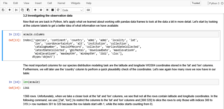
While Jupyter Notebook has been developed within the Python ecosystem, it can be used with other programming languages, for instance, the R language that you at least may have heard about as one of the main languages used for statistical computing. One of the things you will see in this lesson is how one can actually combine Python and R code within a Jupyter notebook to realize a somewhat complex spatial data science project in the area of species distribution modeling, also termed ecological niche modeling.
It may be interesting for you to know that Esri is also supporting Jupyter Notebook as a platform for conducting GIS projects with the help of their ArcGIS API for Python library and Jupyter Notebook has been integrated into several Esri products including ArcGIS Pro.
After a quick look at the Python packages most commonly used in the context of data science projects, we will provide a more detailed overview on what is coming in the remainder of the lesson, so that you will be able to follow along easily without getting confused by all the different software packages we are going to use.
3.5.1 Python packages for (spatial) Data Science
It would be impossible to introduce or even just list all the packages available for conducting spatial data analysis projects in Python here, so the following is just a small selection of those that we consider most important.
numpy
numpy (Python numpy page, Wikipedia numpy page) stands for “Numerical Python” and is a library that adds support for efficiently dealing with large and multi-dimensional arrays and matrices to Python together with a large number of mathematical operations to apply to these arrays, including many matrix and linear algebra operations. Many other Python packages are built on top of the functionality provided by numpy.
matplotlib
matplotlib (Python matplotlib page, Wikipedia matplot page) is an example of a Python library that builds on numpy. Its main focus is on producing plots and embedding them into Python applications. Take a quick look at its Wikipedia page to see a few examples of plots that can be generated with matplotlib. We will be using matplotlib a few times in this lesson’s walkthrough to quickly create simple map plots of spatial data.
SciPy
SciPy (Python SciPy page, Wikipedia SciPy page) is a large Python library for application in mathematics, science, and engineering. It is built on top of both numpy and matplotlib, providing methods for optimization, integration, interpolation, signal processing and image processing. Together numpy, matplotlib, and SciPy roughly provide a similar functionality as the well known software Matlab. While we won’t be using SciPy in this lesson, it is definitely worth checking out if you're interested in advanced mathematical methods.
pandas
pandas (Python pandas page, Wikipedia pandas software page) provides functionality to efficiently work with tabular data, so-called data frames, in a similar way as this is possible in R. Reading and writing tabular data, e.g. to and from .csv files, manipulating and subsetting data frames, merging and joining multiple data frames, and time series support are key functionalities provided by the library. A more detailed overview on pandas will be given in Section 3.8.
Shapely
Shapely (Python Shapely page, Shapely User Manual) adds the functionality to work with planar geometric features in Python, including the creation and manipulation of geometries such as points, polylines, and polygons, as well as set-theoretic analysis capabilities (intersection, union, …). It is based on the widely used GEOS library, the geometry engine that is used in PostGIS, which in turn is based on the Java Topology Suite (JTS) and largely follows the OGC’s Simple Features Access Specification.
geopandas
geopandas (Python geopandas page, GeoPandas page) combines pandas and Shapely to facilitate working with geospatial vector data sets in Python. While we will mainly use it to create a shapefile from Python, the provided functionality goes significantly beyond that and includes geoprocessing operations, spatial join, projections, and map visualizations.
GDAL/OGR
GDAL/OGR (Python GDAL page, GDAL/OGR Python) is a powerful library for working with GIS data in many different formats widely used from different programming languages. Originally, it consisted of two separated libraries, GDAL (‘Geospatial Data Abstraction Library‘) for working with raster data and OGR (used to stand for ‘OpenGIS Simple Features Reference Implementation’) for working with vector data, but these have now been merged. The gdal Python package provides an interface to the GDAL/OGR library written in C++. In Section 3.9 and the lesson’s walkthrough, you will see some examples of applying GDAL/OGR.
ArcGIS API for Python
As we already mentioned at the beginning, Esri provides its own Python API (ArcGIS for Python page) for working with maps and GIS data via their ArcGIS Online and Portal for ArcGIS web platforms. The API allows for conducting administrative tasks, performing vector and raster analyses, running geocoding tasks, creating map visualizations, and more. While some services can be used autonomously, many are tightly coupled to Esri’s web platforms and you will at least need a free ArcGIS Online account. The Esri API for Python will be further discussed in Section 3.10.
3.5.2 The lesson in more detail
In this lesson, we will start to work with some software that you probably are not familiar with and we will be using Python packages extensively that we have not used before to demonstrate how a complex GIS project can be solved in Python by combining different languages and packages within a Jupyter Notebook. Therefore, it is probably a good idea to prepare you a bit with an overview of what will happen in the remainder of the lesson.
- We already discussed the idea of using Jupyter Notebooks for data analysis projects. We will start this part of the lesson by introducing you to Jupyter Notebook and explaining to you the basic functionality (Section 3.6) so that you will be able to use it for the remainder of the lesson and future Python projects.
- The R programming language has its roots in statistical computing but also comes with a large library of packages providing data analysis methods for many specialized areas. One such package is the ‘dismo’ package for species distribution modeling. We will use the task of generating a species distribution model for the Solanum Acaule plant species as the data analysis task for this lesson’s walkthrough with the goal of showing you how Python and R functions can be combined within a Jupyter Notebook to solve some pretty complex analysis problem. The species distribution modeling application will be discussed further together with a brief overview on R and the ‘dismo’ package in Section 3.7.
- Using pandas for the manipulation of tabular data will be a significant part of this lesson’s walkthrough. We will use it to clean up the somewhat messy observation data available for Solanum Acaule. As a preparation, we will teach you the basics of manipulating table data with pandas in Section 3.8.
- GDAL/OGR will be the main geospatial extension of Python that we will use in this lesson (a) to perform additional data cleaning based on spatial querying and (b) to prepare additional input data (raster data sets for different climatic variables). We, therefore, provide an overview on its functionality and typical patterns of using GDAL/OGR in Section 3.9.
- We will mainly use the Esri ArcGIS API for Python to create an interactive map visualization within a Jupyter Notebook. However, the API has much more to offer and provides an interesting bridge between the FOSS Python Data Science ecosystem and the proprietary Esri world. We, therefore, provide an overview of the API in Section 3.10.
- The lesson’s walkthrough in Section 3.11 will show you a solution to the task of creating a species distribution model for Solanum Acaule combining both Python and R and making use of the different Python packages introduced in the lesson. The walkthrough will be provided as a Jupyter notebook that you can download and run on your own computer.
3.6 Jupyter Notebook
As we already explained, the idea of a Jupyter Notebook is that it can contain code, the output produced by the code, and rich text that, like in a normal text document, can be styled and include images, tables, equations, etc. Jupyter Notebook is a client-server application meaning that the core Jupyter program can be installed and run locally on your own computer or on a remote server. In both cases, you communicate with it via your web browser to create, edit, and execute your notebooks.
The history of Jupyter Notebook goes back to the year 2001 when Fernando Pérez started the development of IPython, a command shell for Python (and other languages) that provides interactive computing functionalites. In 2007, the IPython team started the development of a notebook system based on IPython for combining text, calculations, and visualizations, and a first version was released in 2011. In 2014, the notebook part was split off from IPython and became Project Jupyter, with IPython being the most common kernel (= program component for running the code in a notebook) for Jupyter but not the only one. There now exist kernels to provide programming language support for Jupyter notebooks for many common languages including Ruby, Perl, Java, C/C++, R, and Matlab.
To get a first impression of Jupyter Notebook have a look at Figure 3.2 (which you already saw earlier). The shown excerpt consists of two code cells with Python code (those with starting with “In [...]:“) and the output produced by running the code (“Out[...]:”), and of three different rich text cells before, after, and between the code cells with explanations of what is happening. The currently active cell is marked by the blue bar on the left and frame around it.
Before we continue to discuss what Jupyter Notebook has to offer, let’s get it running on your computer so that you can directly try out the examples.
3.6.1 Running Jupyter Notebook
Juypter Notebook is already installed in the Anaconda environment AC36 or AC37 we created in Section 3.2. If you have the Anaconda Navigator running, make sure it shows the “Home” page and that our AC36 or AC37 environment is selected. Then you should see an entry for Juypter Notebook with a Launch button (Figure 3.3). Click the ‘Launch’ button to start up the application. This will ensure that your notebook starts with the correct environment. Starting Jupyter Notebook this way will create the link to shortcuts for a Jupyter Notebook to that conda environment so you can use it in the way we describe below.
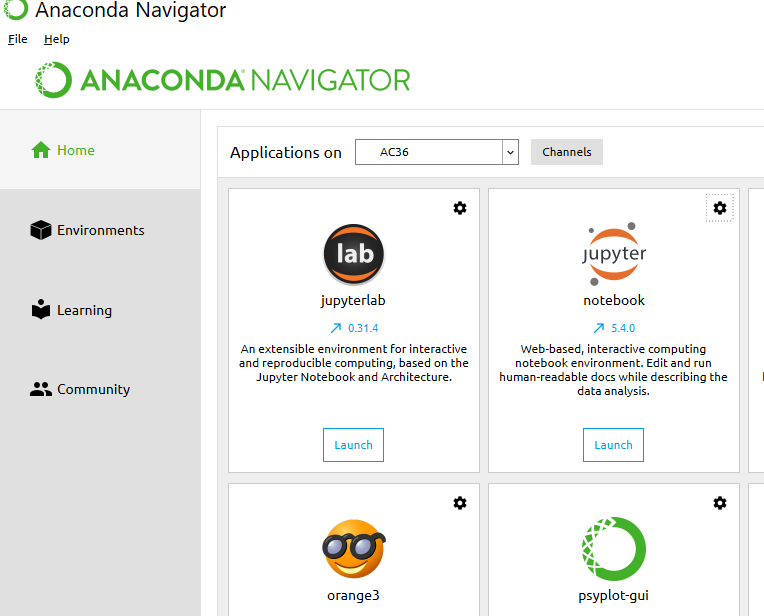
Alternatively, you can start up Jupyter directly without having to open Anaconda first: You will find the Juypter Notebook application in your Windows application list as a subentry of Anaconda. Be sure that you start the Jupyter Notebook for the recently created conda environment (which will only be created if you change the dropdown in Anaconda Navigator above). Alternatively, simply press the Windows key and then type in the first few characters of Jupyter until Jupyter (with the correct conda environment) shows up in the search results.
When you start up Jupyter, two things will happen: The server component of the Jupyter application will start up in a Windows command line window showing log messages, e.g. that the server is running locally under the address http://localhost:8888/ (see Figure 3.4 (a)). When you start Jupyter from the Anaconda Navigator, this will actually happen in the background and you won't get to see the command line window with the server messages. In addition, the web-based client application part of Jupyter will open up in your standard web browser showing you the so-called Dashboard, the interface for managing your notebooks, creating new ones, and also managing the kernels. Right now it will show you the content of the default Jupyter home folder, which is your user’s home folder, in a file browser-like interface (Figure 3.4 (b)).
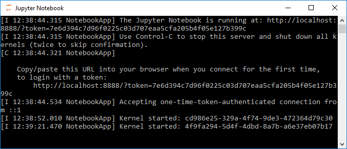
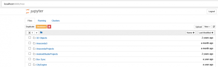
The file tree view allows you to navigate to existing notebooks on your disk, to open them, and to create new ones. Notebook files will have the file extension .ipynb . Let’s start by creating a new notebook file to try out the things shown in the next sections. Click the ‘New…’ button at the top right, then choose the ‘Python 3’ option. A new tab will open up in your browser showing an empty notebook page as in Figure 3.5.
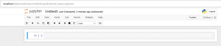
Before we are going to explain how to edit and use the notebook page, please note that the page shows the title of the notebook above a menu bar and a toolbar that provide access to the main operations and settings. Right now, the notebook is still called ‘Untitled...’, so, as a last preparation step, let’s rename the notebook by clicking on the title at the top and typing in ‘MyFirstJupyterNotebook’ as the new title and then clicking the ‘Rename’ button (Figure 3.6).
If you go back to the still open ‘Home’ tab with the file tree view in your browser, you can see your new notebook listed as MyFirstJupyterNotebook.ipynb and with a green ‘Running’ tag indicating that this notebook is currently open. You can also click on the ‘Running’ tab at the top to only see the currently opened notebooks (the ‘Clusters’ tab is not of interest for us at the moment). Since we created this notebook in the Juypter root folder, it will be located directly in your user’s home directory. However, you can move notebook files around in the Windows File Explorer if, for instance, you want the notebook to be in your Documents folder instead. To create a new notebook directly in a subfolder, you would first move to that folder in the file tree view before you click the ‘New…’ button.

3.6.2 First steps to editing a Jupyter Notebook
We will now explain the basics of editing a Jupyter Notebook. We cannot cover all the details here, so if you enjoy working with Jupyter and want to learn all it has to offer as well as all the little tricks that make life easier, the following resources may serve as good starting points:
- Jupyter Documentation
- The Jupyter Notebook
- 28 Jupyter Notebook tips, tricks, and shortcuts
- Jupyter Notebook Tutorial: The Definitive Guide
A Jupyter notebook is always organized as a sequence of so called ‘cells’ with each cell either containing some code or rich text created using the Markdown notation approach (further explained in a moment). The notebook you created in the previous section currently consists of a single empty cell marked by a blue bar on the left that indicates that this is the currently active cell and that you are in ‘Command mode’. When you click into the corresponding text field to add or modify the content of the cell, the bar color will change to green indicating that you are now in ‘Edit mode’. Clicking anywhere outside of the text area of a cell will change back to ‘Command mode’.
Let’s start with a simple example for which we need two cells, the first one with some heading and explaining text and the second one with some simple Python code. To add a second cell, you can simply click on the  symbol. The new cell will be added below the first one and become the new active cell shown by the blue bar (and frame around the cell’s content). In the ‘Insert’ menu at the top, you will also find the option to add a new cell above the currently active one. Both adding a cell above and below the current one can also be done by using the keyboard shortcuts ‘A’ and ‘B’ while in ‘Command mode’. To get an overview on the different keyboard shortcuts, you can use Help -> Keyboard Shortcuts in the menu at the top.
Both cells that we have in our notebook now start with “In [ ]:” in front of the text field for the actual cell content. This indicates that these are ‘Code’ cells, so the content will be interpreted by Jupyter as executable code. To change the type of the first cell to Markdown, select that cell by clicking on it, then change the type from ‘Code’ to ‘Markdown’ in the dropdown menu  in the toolbar at the top. When you do this, the “In [ ]:” will disappear and your notebook should look similar to Figure 3.8 below. The type of a cell can also be changed by using the keyboard shortcuts ‘Y’ for ‘Code’ and ‘M’ for ‘Markdown’ when in ‘Command mode’.

Let’s start by putting some Python code into the second(!) cell of our notebook. Click on the text field of the second cell so that the bar on the left turns green and you have a blinking cursor at the beginning of the text field. Then enter the following Python code:
from bs4 import BeautifulSoup
import requests

documentURL = 'https://www.e-education.psu.edu/geog489/l1.html'

html = requests.get(documentURL).text
soup = BeautifulSoup(html, 'html.parser')

print(soup.get_text())
This brief code example is similar to what you already saw in Lesson 2. It uses the requests Python package to read in the content of an html page from the URL that is provided in the documentURL variable. Then the package BeautifulSoup4 (bs4) is used for parsing the content of the file and we simply use it to print out the plain text content with all tags and other elements removed by invoking its get_text() method in the last line.
While Jupyter by default is configured to periodically autosave the notebook, this would be a good point to explicitly save the notebook with the newly added content. You can do this by clicking the disk  symbol or simply pressing ‘S’ while in ‘Command mode’. The time of the last save will be shown at the top of the document, right next to the notebook name. You can always revert back to the last previously saved version (also referred to as a ‘Checkpoint’ in Jupyter) using File -> Revert to Checkpoint. Undo with CTRL-Z works as expected for the content of a cell while in ‘Edit mode’; however, you cannot use it to undo changes made to the structure of the notebook such as moving cells around. A deleted cell can be recovered by pressing ‘Z’ while in ‘Command mode’ though.
Now that we have a cell with some Python code in our notebook, it is time to execute the code and show the output it produces in the notebook. For this you simply have to click the run  symbol button or press ‘SHIFT+Enter’ while in ‘Command mode’. This will execute the currently active cell, place the produced output below the cell, and activate the next cell in the notebook. If there is no next cell (like in our example so far), a new cell will be created. While the code of the cell is being executed, a * will appear within the squared brackets of the “In [ ]:”. Once the execution has terminated, the * will be replaced by a number that always increases by one with each cell execution. This allows for keeping track of the order in which the cells in the notebook have been executed.
Figure 3.9 below shows how things should look after you executed the code cell. The output produced by the print statement is shown below the code in a text field with a vertical scrollbar. We will later see that Jupyter provides the means to display other output than just text, such as images or even interactive maps.
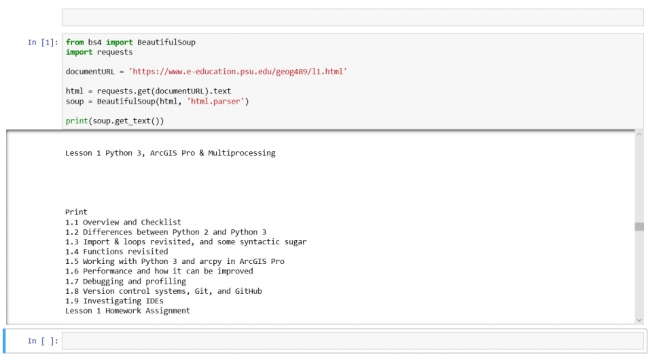
In addition to running just a single cell, there are also options for running all cells in the notebook from beginning to end (Cell -> Run All) or for running all cells from the currently activated one until the end of the notebook (Cell -> Run All Below). The produced output is saved as part of the notebook file, so it will be immediately available when you open the notebook again. You can remove the output for the currently active cell by using Cell -> Current Outputs -> Clear, or of all cells via Cell -> All Output -> Clear.
Let’s now put in some heading and information text into the first cell using the Markdown notation. Markdown is a notation and corresponding conversion tool that allows you to create formatted HTML without having to fiddle with tags and with far less typing required. You see examples of how it works by going Help -> Markdown in the menu bar and then clicking the “Basic writing and formatting syntax” link on the web page that opens up. This page here also provides a very brief overview on the markdown notation. If you browse through the examples, you will see that a first level heading can be produced by starting the line with a hashmark symbol (#). To make some text appear in italics, you can delimit it by * symbols (e.g., *text*), and to make it appear in bold, you would use **text** . A simple bullet point list can be produced by a sequence of lines that start with a – or a *.
Let’s say we just want to provide a title and some bullet point list of what is happening in this code example. Click on the text field of the first cell and then type in:
# Simple example of reading a web page and converting it to plain text
How the code works:
* package **requests** is used to load web page from URL given in variable *documentURL*
* package **BeautifulSoup4 (bs4)** is used to parse content of loaded web page
* the call of *soup.get_text()* in the last line provides the content of page as plain text
While typing this in, you will notice that Jupyter already interprets the styling information we are providing with the different notations, e.g. by using a larger blue font for the heading, by using bold font for the text appearing within the **…**, etc. However, to really turn the content into styled text, you will need to ‘run the cell’ (SHIFT+Enter) like you did with the code cell. As a result, you should get the nicely formatted text shown in Figure 3.10 below that depicts our entire first Jupyter notebook with text cell, code cell, and output. If you want to see the Markdown code and edit it again, you will have to double-click the text field or press ‘Enter’ to switch to ‘Edit mode’.
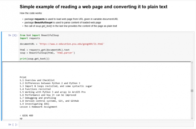
If you have not worked with Markdown styling before, we highly recommend that you take a moment to further explore the different styling options from the “Basic writing and formatting syntax” web page. Either use the first cell of our notebook to try out the different notations or create a new Markdown cell at the bottom of the notebook for experimenting.
This little example only covered the main Jupyter operations needed to create a first Jupyter notebook and run the code in it. The ‘Edit’ menu contains many operations that will be useful when creating more complex notebooks, such as deleting, copying, and moving of cells, splitting and merging functionality, etc. For most of these operations, there also exist keyboard shortcuts. If you find yourself in a situation in which you can’t figure out how to use any of these operations, please feel free to ask on the forums.
3.6.3 Magic commands
Jupyter provides a number of so-called magic commands that can be used in code cells to simplify common tasks. Magic commands are interpreted by Jupyter and, for instance, transformed into Python code before the content is passed on to the kernel for execution. This happens behind the scenes, so you will always only see the magic command in your notebook. Magic commands start with a single % symbol if they are line-oriented meaning they should be applied to the remaining content of the line, and with %% if they are cell-oriented meaning they should be applied to the rest of the cell. As a first example, you can use the magic command %lsmagic to list the available magic commands (Figure 3.11). To get the output you have to execute the cell as with any other code cell.
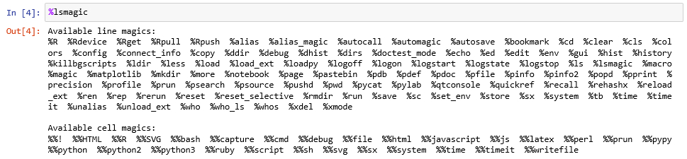
The %load_ext magic command can be used for loading IPython extension which can add new magic commands. The following command loads the IPython rpy2 extension. If that code gives you a long list of errors then the rpy2 package isn't installed and you will need to go back to Section 3.2 and follow the instructions there.
We recently had cases where loading rpy2 failed on some systems due to the R_HOME environment variable not being set correctly. We therefore added the first line below which you will have to adapt to point to the lib\R folder in your AC Python environment.
import os, rpy2
os.environ['R_HOME'] = r'C:\Users\username\anaconda3\envs\AC37\lib\R' # workaround for R.dll issue occurring on some systems
%load_ext rpy2.ipython
Using a ? symbol in front of a magic command will open a subwindow with the documentation of that command at the bottom of the browser window. Give it a try by executing the command
?%Rin a cell. %R is a magic command from the rpy2 extension that we just loaded and the documentation will tell you that this command can be used to execute some line of R code that follows the %R and optionally pass variable values between the Python and R environments. We will use this command several times in the lesson’s walkthrough to bridge between Python and R. Keep in mind that it is just an abbreviation that will be replaced with a bunch of Python statements by Jupyter. If you would want the same code to work as a stand-alone Python script outside of Jupyter, you would have to replace the magic command by these Python statements yourself. You can also use the ? prefix to show the documentation of Python elements such as classes and functions, for instance by writing
?BeautifulSoup
or
?soup.get_text()
Give it a try and see if you understand what the documentation is telling you.
3.6.4 Widgets
Jupyter notebooks can also include interactive elements, referred to as widgets as in Lesson 2, like buttons, text input fields, sliders, and other GUI elements, as well as visualizations, plots, and animations. Figure 3.12 shows an example that places three button widgets and then simply prints out which button has been pressed when you click on them. The ipywidgets and IPython.display packages imported at the beginning are the main packages required to place the widgets in the notebook. We then define a function that will be invoked whenever one of the buttons is clicked. It simply prints out the description attribute of the button (b.description). In the for-loop we create the three buttons and register the onButtonClick function as the on_click event handler function for all of them.
from ipywidgets import widgets
from IPython.display import display

def onButtonClick(b):
    print("Button " + b.description + " has been clicked")

for i in range(1,4):
    button = widgets.Button(description=str(i))
    display(button)
    button.on_click(onButtonClick)
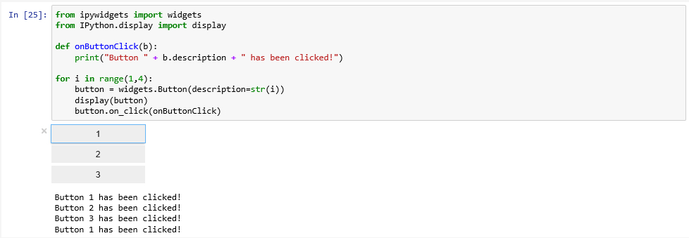
If you get an error with this code "Failed to display Jupyter Widget of type Button" that means the widgets are probably not installed which we can potentially fix in our Anaconda prompt:
conda install -n base -c conda-forge widgetsnbextension
conda install -n AC37 -c conda-forge ipywidgets
After installing the packages, exit your Jupyter notebook and restart it and try to re-run your code. It's possible you will receive the error again as the widget tries to run before the Javascript library that runs the widgets has opened. In that case try to select your code, wait a few more seconds and then click Run.
If you're still getting an error, it's likely that your packages didn't install properly (or in a way that Jupyter/Anaconda could find them). The fix for this is to close Jupyter Notebook, return to Anaconda Navigator, click Environments (on the left), choose your environment and then search for "ipy", you may need to either change the "Installed" dropdown to "Not Installed" if they are missing or perhaps they should be updated (by clicking on the upward point arrow or the blue text).
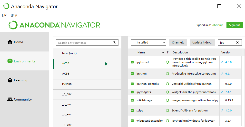
It is easy to imagine how this example could be extended to provide some choices on how the next analysis step in a longer Data Science project should be performed. Similarly, a slider or text input field could be used to allow the notebook user to change the values of important input variables.
3.6.5 Autocompletion, restarting the kernel, and other useful things
Let’s close this brief introduction to Jupyter with a few more things that are good to know when starting to write longer and more complex notebooks. Like normal development environments, Juypter has an autocomplete feature that helps with the code writing and can save a lot of typing: while editing code in a code cell, you can press the TAB key and Jupyter will either automatically complement the name or keyword you are writing or provide you with a dropdown list of choices that you can pick from. For instance, type in soup.ge and then press TAB and you get the list of options, as shown in Figure 3.13 including the get_text() function that we used in our code.
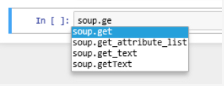
Another useful keyboard command to remember is SHIFT+TAB. When you place the cursor on a variable name or function call and press this key combination, a window will open up showing helpful information like the type of the variable and its current content or the parameters of the function as in Figure 3.14. This is of great help if you are unsure about the different parameters of a function, their order or names. Try out what you get when you use this key combination for different parts of the code in this notebook.
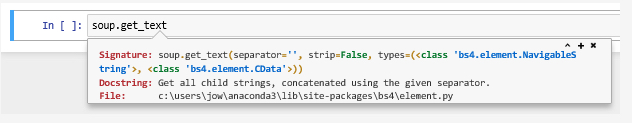
As in all programming, it may occasionally happen that something goes completely wrong and the execution of the code in a cell won’t terminate in the expected time or not at all. If that happens, the first thing to try is to use the “Interrupt Kernel” button located to the right of the “Execute cell” button. This should stop the execution of the current cell and you can then modify the code and try to run the cell again. However, sometimes even that won’t help because the kernel has become unresponsive. In that case, the only thing you can do is restart the kernel using the “Restart Kernel” button to the right of the “Interrupt Kernel” button. Unfortunately, that means that you will have to start the execution of the code in your notebook from the beginning because all imports and variable assignments will be lost after the restart.
Once you have finished your notebook, you may want to publish or share it. There are many options by wich to do so. In the File menu, there exists the “Download as…” option for obtaining versions of your notebook in different formats. The .ipynb format, as we mentioned, is the native format in which Jupyter saves the notebooks. If you make the .ipynb file available to someone who has access to Juypter, that person can open the notebook and run it or modify the content. The .py option allows for exporting content as a Python script, so that the code can be run outside of Jupyter. If you want a version of your notebook that others can read even without access to Jupyter, there are several options like exporting the notebook as HTML, as Latex, or as PDF. Some of these options require additional software tools to be installed on your computer and there are some limitations. For instance, if you export your notebook as HTML to add it to your personal web page, interactive widgets such as the interactive web map you will see later in Section 3.10 will not be included.
To close this section, we want to again refer to the links we provided at the beginning of Section 3.6.2 if you want to keep reading about Jupyter and learn tricks that we weren't able to cover in this brief introduction. In the remainder of this lesson, please use Jupyter to try out the code examples by entering them into a Jupyter notebook and running the code there to get some more practice with Jupyter.
3.7 Species distribution modeling with R and the dismo package
Before we will start to create another Jupyter notebook with a much more complex example, let us talk about the task and application domain we will be using. As we mentioned at the beginning of the lesson, we will be using a Jupyter notebook to connect Python with R to be able to use some specialized statistical models for the application field of species distribution modeling.
Simply speaking, species distribution modeling is the task or process of predicting the real-world distribution or likelihood of a species occurring at any location on the earth based on (a) existing occurrence and potentially also absence data, e.g. from biological surveys, and (b) data for a number of predictive variables, most often climate related, but also including elevation, soil type, land cover type, etc. The output of a species distribution model is typically a raster with probabilities for the area of interest (which might be the entire earth) that can be used to create a map visualization to help with analysis and decision making. Anticipating the main result of this lesson’s walkthrough, Figure 3.15(b) shows the distribution of Solanum acaule, a plant species growing in the western countries of South America, as predicted by a particular species distribution model that is implemented in the R package ‘dismo’ developed and maintained by Robert J. Hijmans and colleagues. The prediction has been created with the Bioclim model which is one of several models available in dismo.
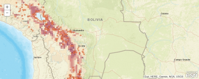
Teaching you the basics of R is beyond the scope of this course, and you really won’t need R knowledge to follow and understand the short pieces of R code we will be using in this lesson’s walkthrough. However, if you have not worked with R before, you may want to take a quick look through the first five sections of this brief R tutorial (or one of the many other R tutorials on the web). Please note that in this lesson we are not trying to create the best possible distribution model for Solanum acaule (and what actually makes a good or optimal model is something that is heavily debated even among experts anyway). Our main goal is to introduce different Python packages and show how they can be combined to solve spatial analysis tasks inside a Jupyter notebook without letting things get too complex. We, therefore, made quite a few simplifications with regard to what input data to use, how to preprocess it, the species distribution model itself, and how it is applied. As a result, the final model created and shown in the figure above should be taken with a grain of salt.
The ‘dismo’ R package contains a collection of different species modeling approaches as well as many auxiliary functions for obtaining and preprocessing data. See the official documentation of the module. The authors have published detailed additional documentation available in this species distribution modeling document that provides examples and application guidelines for the package and that served as a direct inspiration for this lesson’s walkthrough. One of the main differences is that we will be doing most of the work in Python and only use R and the ‘dismo’ package to obtain some part of the input data and later apply a particular species modeling approach to this data.
Species distribution modeling approaches can roughly be categorized into methods that only use presence data and methods that use both presence and absence data as well as into regression and machine learning based methods. The ‘dismo’ package provides implementations of various models from these different classes but we will only use a rather simple one, the Bioclim model, in this lesson. Bioclim only uses presence data and looks at how close the values of given environmental predictor variables (provided as raster files) for a particular location are to the median values of these variables over the locations where the species has been observed. Because of its simplicity, Bioclim is particularly well suited for teaching purposes.
The creation of a prediction typically consists of the following steps:
- Obtaining and preprocessing of all input data (species presence/absence data and data for environmental predictor variables)
- Creation of the model from the input data
- Using the model to create a prediction based on data for the predictor variables.
require('dismo')
bc <- bioclim(predictorRasters, observationPoints)
You can then use the model to create a Bioclim prediction raster and store it in variable pb and create a plot of the raster with the following R code:
pb <- predict(predictorRasters, bc)
plot(pb, main='Bioclim, raw values')
You may be wondering how you can actually use R commands from inside your Python code. We already mentioned that the magic command %R (or %%R for the cell-oriented version) can be used to invoke R commands within a Python Jupyter notebook. The connection via Python and R is implemented by the rpy2 package that allows for running R inside a Python process. We cannot go into the details of how rpy2 works and how one would use it outside of Jupyter here, so we will just focus on the usage via the %R magic command. To prepare your Jupyter Notebook to interface with R, you will always first have to run the magic command
%load_ext rpy2.ipython
... to load the IPhython rpy2 extension. (If you are trying this out and get an error message about being unable to load the R.dll library, use the following command to manually define the R_HOME environment variable, put in your Windows user ID, and make sure it points to the R folder in your Anaconda AC36/37 environment: os.environ['R_HOME'] = r'C:\Users\youruserid\anaconda3\envs\AC37\lib\R' )
We can then simply execute a single R command by using
%R <command>
To transfer the content of a Python variable to R, we can use
%R –i <name of Python variable>
This creates an R variable with the same name as the Python variable and an R version of the content assigned to it. Similarly,
%R –o <name of R variable>
...can be used for the other direction, so for creating a Python variable with the same name and content as a given R variable. As we will further see in the lesson’s walkthrough, these steps combined make it easy to use R inside a Python Jupyter notebook. However, one additional important component is needed: in R most data used comes in the form of so-called data frames, spreadsheet-like data objects in tabular form in which the content is structured into rows, columns, and cells. R provides a huge collection of operations to read, write, and manipulate data frames. Can we find something similar on the Python side as well that will allow us to work with tabular data (such as attribute information for a set of spatial features) directly in Python? The answer is yes, and the commonly used package to work with tabular data in Python is pandas, so we will talk about it next.
3.8 Pandas and the manipulation of tabular data
The pandas package provides high-performance data structures and analysis tools, in particular for working with tabular data based on a fast and efficient implementation of a data frame class. It also allows for reading and writing data from/to various formats including CSV and Microsoft Excel. In the following, we show you some examples illustrating how to perform the most important data frame related operations with pandas. Again, we can only scratch the surface of the functionality provided by pandas here. Resources provided at the end will allow you to dive deeper if you wish to do so. We recommend that you start a new Jupyter Notebook and use it to try out the examples from this section for yourself. Use a new code cell for each of block of code you will encounter on the following pages.
3.8.1 Creating a new data frame
In our examples, we will be using pandas in combination with the numpy package, the package that provides many fundamental scientific computing functionalities for Python and that many other packages are built on. So we start by importing both packages:
import pandas as pd
import numpy as np
A data frame consists of cells that are organized into rows and columns. The rows and columns have names that serve as indices to access the data in the cells. Let us start by creating a data frame with some random numbers that simulate a time series of different measurements (columns) taken on consecutive days (rows) from January 1, 2017 to January 6, 2017. The first step is to create a pandas series of dates that will serve as the row names for our data frame. For this, we use the pandas function date_range(…):
dates = pd.date_range('20170101' , periods=6, freq='D')
dates
The first parameter given to date_range is the starting date. The ‘periods’ parameter tells the function how many dates we want to generate, while we use ‘freq’ to tell it that we want a date for every consecutive day. If you look at the output from the second line we included, you will see that the object returned by the function is a DatetimeIndex object which is a special class defined in pandas.
Next, we generate random numbers that should make up the content of our date frame with the help of the numpy function randn(…) for creating a set of random numbers that follow a standard normal distribution:
numbers = np.random.randn(6,4) numbers
The output is a two-dimensional numpy array of random numbers normally distributed around 0 with 4 columns and 6 rows. We create a pandas data frame object from it with the following code:
df = pd.DataFrame(numbers, index=dates, columns=['m1', 'm2', 'm3', 'm4']) df
Note that we provide our array of random numbers as the first parameter, followed by the DatetimeIndex object we created earlier for the row index. For the columns, we simply provide a list of the names with ‘m1’ standing for measurement 1, ‘m2’ standing for measurement 2, and so on. Please also note how the resulting data frame is displayed as a nicely formatted table in your Jupyter Notebook because it makes use of IPython widgets. Please keep in mind that because we are using random numbers for the content of the cells, the output produced by commands used in the following examples will look different in your notebook because the numbers are different.
3.8.2 Subsetting and changing cell values
Now that we have a data frame object available, let’s quickly go through some of the basic operations that one can perform on a data frame to access or modify the data.
The info() method can be used to display some basic information about a data frame such as the number of rows and columns and data types of the columns:
df.info()
The output tells us that we have four columns, all for storing floating point numbers, and each column has 6 rows with values that are not null. If you ever need the number of rows and columns, you can get them by applying the len(…) operation to the data frame and to the columns property of the data frame:
print(len(df)) # gives you the number of rows print(len(df.columns)) # gives you the number of columns
We can use the head(…) and tail(…) methods to get only the first or last n rows of a data frame:
firstRows = df.head(2) print(firstRows) lastRows = df.tail(2) print(lastRows)
We can also just get a subset of consecutive rows by applying slicing to the data frame similar to how this can be done with lists or strings:
someRows = df[3:5] # gives you the 4th and 5th row print(someRows)
This operation gives us rows 4 and 5 (those with index 3 and 4) from the original data frame because the second number used is the index of the first row that will not be included anymore.
If we are just interested in a single column, we can get it based on its name:
thirdColumn = df.m3 print(thirdColumn)
The same can be achieved by using the notation df['m3'] instead of df.m3 in the first line of code. Moreover, instead of using a single column name, you can use a list of column names to get a data frame with just these columns and in the specified order:
columnsM3andM2 = df[ ['m3', 'm2'] ] columnsM3andM2
| m3 | m2 | |
|---|---|---|
| 2017-01-01 | 0.510162 | 0.163613 |
| 2017-01-02 | 0.025050 | 0.056027 |
| 2017-01-03 | -0.422343 | -0.840010 |
| 2017-01-04 | -0.966351 | -0.721431 |
| 2017-01-05 | -1.339799 | 0.655267 |
| 2017-01-06 | -1.160902 | 0.192804 |
The column subsetting and row slicing operations shown above can be concatenated into a single expression. For instance, the following command gives us columns ‘m3’ and ‘m2’ and only the rows with index 3 and 4:
someSubset = df[['m3', 'm2']][3:5] someSubset
The order here doesn’t matter. We could also have written df[3:5][['m3', 'm2']] .
The most flexible methods for creating subsets of data frame are via the loc and .iloc index properties of a data frame. .iloc[…] is based on the numerical indices of the columns and rows. Here is an example:
someSubset = df.iloc[2:4,1:3] print(someSubset)
The part before the comma determines the rows (rows with indices 2 and 3 in this case) and the part after the comma, the columns (columns with indices 1 and 2 in this case). So we get a data frame with the 3rd and 4th rows and 2nd and 3rd columns of the original data frame. Instead of slices we can also use lists of row and column indices to create completely arbitrary subsets. For instance, using iloc in the following example
someSubset = df.iloc[ [0,2,4], [1,3] ] print(someSubset)
...gives us a data frame with the 1st, 3rd, and 5th row and 2nd and 4th column of the original dataframe. Both the part before the comma and after the comma can just be a colon symbol (:) in which case all rows/columns will be included. For instance,
allRowsSomeColumns = df.iloc[ : , [1,3] ] print(allRowsSomeColumns)
...will give you all rows but only the 2nd of 4th column.
In contrast to iloc, loc doesn’t use the row and column numbers but instead is based on their labels, while otherwise working in the same way as iloc. The following command produces the same subset of the 1st, 3rd, and 5th rows and 2nd and 4th columns as the iloc code from two examples above:
someSubset = df.loc[ [pd.Timestamp('2017-01-01'), pd.Timestamp('2017-01-03'), pd.Timestamp('2017-01-05')] , ['m2', 'm4'] ]
print(someSubset)
Please note that, in this example, the list for the column names at the very end is simply a list of strings but the list of dates for the row names has to consist of pandas Timestamp objects. That is because we used a DatetimeIndex for the rows when we created the original data frame. When a data frame is displayed, the row names show up as simple strings but they are actually Timestamp objects. However, a DatetimeIndex for the rows has many advantages; for instance, we can use it to get all rows for dates that are from a particular year, e.g. with
df.loc['2017' , ['m2', 'm4'] ]
...to get all dates from 2017 which, of course, in this case, are all rows. Without going into further detail here, we can also get all dates from a specified time period, etc.
The methods explained above for accessing subsets of a data frame can also be used as part of an assignment to change the values in one or several cells. In the simplest case, we can change the value in a single cell, for instance with
df.iloc[0,0] = 0.17
...or
df.loc['2017-01-01', 'm1'] = 0.17
...to change the value of the top left cell to 0.17. Please note that this operation will change the original data frame, not create a modified copy. So if you now print out the data frame with
df
you will see the modified value for 'm1' of January 1, 2017. Even more importantly, if you have used the operations explained above for creating a subset, the data frame with the subset will still refer to the original data, so changing a cell value will change your original data. If you ever want to make changes but keep the original data frame unchanged, you need to explicitly make a copy of the data frame by calling the copy() method as in the following example:
dfCopy = df.copy() dfCopy.iloc[0,0] = 0 print(df) print(dfCopy)
Check out the output and compare the top left value for both data frames. The data frame in df still has the old value of 0.17, while the value will be changed to 0 in dfCopy. Without using the copy() method in the first line, both variables would still refer to the same underlying data and both would show the 0 value. Here is another slightly more complicated example where we change the values for the first column of the 1st and 5th rows to 1.2 (intentionally modifying the original data):
df.iloc[ [0,4] , [0] ] = 1.2 print(df)
If you ever need to explicitly go through the rows in a data frame, you can do this with a for-loop that uses the itertuples(…) method of the data frame. itertuples(…) gives you an object that can be used to iterate through the rows as named tuples, meaning each element in the tuple is labeled with the respective column name. By providing the parameter index=False to the method, we are saying that we don’t want the row name to be part of the tuple, just the cell values for the different columns. You can access the elements of the tuple either via their index or via the column name:
for row in df.itertuples(index=False):
print(row) # print entire row tuple
print(row[0]) # print value from column with index 0
print(row.m2) # print value from column with name m2
print('----------')
Try out this example and have a look at the named tuple and the output produced by the other two print statements.
3.8.3 Sorting
Pandas also provides operations for sorting the rows in a data frame. The following command can be used to sort our data frame by the values in the ‘m2’ column in decreasing order:
dfSorted = df.sort_values(by='m2', ascending=False) dfSorted
| m1 | m2 | m3 | m4 | m5 | |
|---|---|---|---|---|---|
| 2017-01-05 | 1.200000 | 0.655267 | -1.339799 | 1.075069 | -0.236980 |
| 2017-01-06 | 0.192804 | 0.192804 | -1.160902 | 0.525051 | -0.412310 |
| 2017-01-01 | 1.200000 | 0.163613 | 0.510162 | 0.628612 | 0.432523 |
| 2017-01-02 | 0.056027 | 0.056027 | 0.025050 | 0.283586 | -0.123223 |
| 2017-01-04 | -0.721431 | -0.721431 | -0.966351 | -0.380911 | 0.001231 |
| 2017-01-03 | -0.840010 | -0.840010 | -0.422343 | 1.022622 | -0.231232 |
The ‘by’ argument specifies the column that the sorting should be based on and, by setting the ‘ascending’ argument to False, we are saying that we want the rows to be sorted in descending rather than ascending order. It is also possible to provide a list of column names for the ‘by’ argument, to sort by multiple columns. The sort_values(...) method will create a new copy of the data frame, so modifying any cells of dfSorted in this example will not have any impact on the data frame in variable df.
3.8.4 Adding / removing columns and rows
Adding a new column to a data frame is very simple when you have the values for that column ready in a list. For instance, in the following example, we want to add a new column ‘m5’ with additional measurements and we already have the numbers stored in a list m5values that is defined in the first line of the example code. To add the column, we then simply make an assignment to df['m5'] in the second line. If a column ‘m5’ would already exist, its values would now be overwritten by the values from m5values. But since this is not the case, a new column gets added under the name ‘m5’ with the values from m5values.
m5values = [0.432523, -0.123223, -0.231232, 0.001231, -0.23698, -0.41231] df['m5'] = m5values df
| m1 | m2 | m3 | m4 | m5 | |
|---|---|---|---|---|---|
| 2017-01-01 | 1.200000 | 0.163613 | 0.510162 | 0.628612 | 0.432523 |
| 2017-01-02 | 0.056027 | 0.056027 | 0.025050 | 0.283586 | -0.123223 |
| 2017-01-03 | -0.840010 | -0.840010 | -0.422343 | 1.022622 | -0.231232 |
| 2017-01-04 | -0.721431 | -0.721431 | -0.966351 | -0.380911 | 0.001231 |
| 2017-01-05 | 1.200000 | 0.655267 | -1.339799 | 1.075069 | -0.236980 |
| 2017-01-06 | 0.192804 | 0.192804 | -1.160902 | 0.525051 | -0.412310 |
For adding new rows, we can simply make assignments to the rows selected via the loc operation, e.g. we could add a new row for January 7, 2017 by writing
df.loc[pd.Timestamp('2017-01-07'),:] = [ ... ]
where the part after the equal sign is a list of five numbers, one for each of the columns. Again, this would replace the values in the case that there already is a row for January 7. The following example uses this idea to create new rows for January 7 to 9 using a for loop:
for i in range(7,10):
df.loc[ pd.Timestamp('2017-01-0'+str(i)),:] = [ np.random.rand() for j in range(5) ]
df
| m1 | m2 | m3 | m4 | m5 | |
|---|---|---|---|---|---|
| 2017-01-01 | 1.200000 | 0.163613 | 0.510162 | 0.628612 | 0.432523 |
| 2017-01-02 | 0.056027 | 0.056027 | 0.025050 | 0.283586 | -0.123223 |
| 2017-01-03 | -0.840010 | -0.840010 | -0.422343 | 1.022622 | -0.231232 |
| 2017-01-04 | -0.721431 | -0.721431 | -0.966351 | -0.380911 | 0.001231 |
| 2017-01-05 | 1.200000 | 0.655267 | -1.339799 | 1.075069 | -0.236980 |
| 2017-01-06 | 0.192804 | 0.192804 | -1.160902 | 0.525051 | -0.412310 |
| 2017-01-07 | 0.768633 | 0.559968 | 0.591466 | 0.210762 | 0.610931 |
| 2017-01-08 | 0.483585 | 0.652091 | 0.183052 | 0.278018 | 0.858656 |
| 2017-01-09 | 0.909180 | 0.917903 | 0.226194 | 0.978862 | 0.751596 |
In the body of the for loop, the part on the left of the equal sign uses loc(...) to refer to a row for the new date based on loop variable i, while the part on the right side simply uses the numpy rand() method inside a list comprehension to create a list of five random numbers that will be assigned to the cells of the new row.
If you ever want to remove columns or rows from a data frame, you can do so by using df.drop(...). The first parameter given to drop(...) is a single column or row name or, alternatively, a list of names that should be dropped. By default, drop(...) will consider these as row names. To indicate these are column names that should be removed, you have to specify the additional keyword argument axis=1 . We will see an example of this in a moment.
3.8.5 Joining data frames
The following short example demonstrates how pandas can be used to merge two data frames based on a common key, so to perform a join operation in database terms. Let’s say we have two tables, one listing capitals of states in the U.S. and one listing populations for each state. For simplicity we just define data frames for these with just entries for two states, Washington and Oregon:
df1 = pd.DataFrame( {'state': ['Washington', 'Oregon'], 'capital': ['Olympia', 'Salem']} )
print(df1)
df2 = pd.DataFrame( {'name': ['Washington', 'Oregon'], 'population':[7288000, 4093000]} )
print(df2)
The two data frames produced by this code look like this:
| capital | state | |
|---|---|---|
| 0 | Olympia | Washington |
| 1 | Salem | Oregon |
| name | population | |
|---|---|---|
| 0 | Washington | 7288000 |
| 1 | Oregon | 4093000 |
We here use a new way of creating a data frame, namely from a dictionary that has entries for each of the columns where the keys are the column names (‘state’ and ‘capital’ in the case of df1, and ‘name’ and ‘population’ in case of df2) and the values stored are lists of the values for that column. We now invoke the merge(...) method on df1 and provide df2 as the first parameter meaning that a new data frame will be produced by merging df1 and df2. We further have to specify which columns should be used as keys for the join operation. Since the two columns containing the state names are called differently, we have to provide the name for df1 through the ‘left_on’ argument and the name for df2 through the ‘right_on’ argument.
merged = df1.merge(df2, left_on='state', right_on='name') merged
The joined data frame produced by the code will look like this:
| capital | state | name | population | |
|---|---|---|---|---|
| 0 | Olympia | Washington | Washington | 7288000 |
| 1 | Salem | Oregon | Oregon | 4093000 |
As you see, the data frames have been merged correctly. However, we do not want two columns with the state names, so, as a last step, we remove the column called ‘name’ with the previously mentioned drop(...) method. As explained, we have to use the keyword argument axis=1 to indicate that we want to drop a column, not a row.
newMerged = merged.drop('name', axis=1)
newMerged
Result:
| capital | state | population | |
|---|---|---|---|
| 0 | Olympia | Washington | 7288000 |
| 1 | Salem | Oregon | 4093000 |
If you print out variable merged, you will see that it still contains the 'name' column. That is because drop(...) doesn't change the original data frame but rather produces a copy with the column/row removed.
3.8.6 Advanced data frame manipulation: Filtering via Boolean indexing
When working with tabular data, it is very common that one wants to do something with particular data entries that satisfy a certain condition. For instance, we may want to restrict our analysis to rows that have a value larger than a given threshold for one of the columns. Pandas provides some powerful methods for this kind of filtering, and we are going to show one of these to you in this section, namely filtering with Boolean expressions.
The first important thing to know is that we can use data frames in comparison expressions, like df > 0, df.m1 * 2 < 0.2, and so on. The output will be a data frame that only contains Boolean values (True or False) indicating whether the corresponding cell values satisfy the comparison expression or not. Let’s try out these two examples:
df > 0
The result is a data frame with the same rows and columns as the original data frame in df with all cells that had a value larger than 0 set to True, while all other cells are set to False:
| m1 | m2 | m3 | m4 | m5 | |
|---|---|---|---|---|---|
| 2017-01-01 | True | True | True | True | True |
| 2017-01-02 | True | True | True | True | False |
| 2017-01-03 | False | False | False | False | False |
| 2017-01-04 | False | False | False | False | True |
| 2017-01-05 | True | True | False | True | False |
| 2017-01-06 | True | True | False | True | False |
| 2017-01-07 | True | True | True | True | True |
| 2017-01-08 | True | True | True | True | True |
| 2017-01-09 | True | True | True | True | True |
df.m1 * 2 < 0.2
Here we are doing pretty much the same thing but only for a single column (‘m1’) and the comparison expression is slightly more complex involving multiplication of the cell values with 2 before the result is compared to 0.2. The result is a one-dimensional vector of True and False values corresponding to the cells of the ‘m1’ column in the original data frame:
| 2017-01-01 | False |
|---|---|
| 2017-01-02 | True |
| 2017-01-03 | True |
| 2017-01-04 | True |
| 2017-01-05 | False |
| 2017-01-06 | False |
| 2017-01-07 | False |
| 2017-01-08 | True |
| 2017-01-09 | True |
| Freq: D, Name: m1, dtype: bool | |
Just to introduce another useful pandas method, we can apply the value_counts() method to get a summary of the values in a data frame telling how often each value occurs:
(df.m1 * 2 < 0.2).value_counts()
The expression in the parentheses will give us a boolean column vector as we have seen above, and invoking its value_counts() method tells us how often True and False occur in this vector. (The actual numbers will depend on the random numbers in your original data frame).
The second important component of Boolean indexing is that we can use Boolean operators to combine Boolean data frames as illustrated in the next example:
v1 = df.m1 * 2 < 0.2 print(v1) v2 = df.m2 > 0 print(v2) print(~v1) print(v1 & v2) print(v1 | v2)
This will produce the following output data frames:
| 2017-01-01 | False |
|---|---|
| 2017-01-02 | True |
| 2017-01-03 | True |
| 2017-01-04 | True |
| 2017-01-05 | False |
| 2017-01-06 | False |
| 2017-01-07 | False |
| 2017-01-08 | True |
| 2017-01-09 | True |
| Frew: D, Name: m1, dtype: bool | |
| 2017-01-01 | True |
|---|---|
| 2017-01-02 | False |
| 2017-01-03 | False |
| 2017-01-04 | True |
| 2017-01-05 | True |
| 2017-01-06 | True |
| 2017-01-07 | True |
| 2017-01-08 | True |
| 2017-01-09 | True |
| Frew: D, Name: m2, dtype: bool | |
| 2017-01-01 | True |
|---|---|
| 2017-01-02 | False |
| 2017-01-03 | False |
| 2017-01-04 | False |
| 2017-01-05 | True |
| 2017-01-06 | True |
| 2017-01-07 | True |
| 2017-01-08 | False |
| 2017-01-09 | False |
| Frew: D, Name: m1, dtype: bool | |
| 2017-01-01 | False |
|---|---|
| 2017-01-02 | True |
| 2017-01-03 | False |
| 2017-01-04 | False |
| 2017-01-05 | False |
| 2017-01-06 | False |
| 2017-01-07 | False |
| 2017-01-08 | True |
| 2017-01-09 | True |
| Frew: D, dtype: bool | |
| 2017-01-01 | True |
|---|---|
| 2017-01-02 | True |
| 2017-01-03 | True |
| 2017-01-04 | True |
| 2017-01-05 | True |
| 2017-01-06 | True |
| 2017-01-07 | True |
| 2017-01-08 | True |
| 2017-01-09 | True |
| Frew: D, dtype: bool | |
What is happening here? We first create two different Boolean vectors using two different comparison expressions for columns ‘m1’ and ‘m2’, respectively, and store the results in variables v1 and v2. Then we use the Boolean operators ~ (not), & (and), and | (or) to create new Boolean vectors from the original ones, first by negating the Boolean values from v1, then by taking the logical AND of the corresponding values in v1 and v2 (meaning only cells that have True for both v1 and v2 will be set to True in the resulting vector), and finally by doing the same but with the logical OR (meaning only cells that have False for both v1 and v2 will be set to False in the result). We can construct arbitrarily complex Boolean expressions over the values in one or multiple data frames in this way.
The final important component is that we can use Boolean vectors or lists to select rows from a data frame. For instance,
df[ [True, False, True, False, True, False, True, False, True] ]
... will give us a subset of the data frame with only every second row:
| m1 | m2 | m3 | m4 | m5 | |
|---|---|---|---|---|---|
| 2017-01-01 | 1.200000 | 0.163613 | 0.510162 | 0.628612 | 0.432523 |
| 2017-01-03 | -0.840010 | -0.840010 | -0.422343 | 1.022622 | -0.231232 |
| 2017-01-05 | 1.200000 | 0.655267 | -1.339799 | 1.075069 | -0.236980 |
| 2017-01-07 | 0.399069 | 0.029156 | 0.937808 | 0.476401 | 0.766952 |
| 2017-01-09 | 0.041115 | 0.984202 | 0.912212 | 0.740345 | 0.148835 |
Taken these three things together means we can use arbitrarily logical expressions over the values in a data frame to select a subset of rows that we want to work with. To continue the examples from above, let’s say that we want only those rows that satisfy both the criteria df.m1 * 2 < 0.2 and df.m2 > 0, so only those rows for which the value of column ‘m1’ times 2 is smaller than 0.2 and the value of column ‘m2’ is larger than 0. We can use the following expression for this:
df[v1 & v2 ]
Or even without first having to define v1 and v2:
df[ (df.m1 * 2 < 0.2) & (df.m2 > 0) ]
Here is the resulting data frame:
| m1 | m2 | m3 | m4 | m5 | |
|---|---|---|---|---|---|
| 2017-01-02 | 0.056027 | 0.056027 | 0.025050 | 0.283586 | -0.123223 |
| 2017-01-08 | 0.043226 | 0.904844 | 0.181999 | 0.253381 | 0.165105 |
| 2017-01-09 | 0.041115 | 0.984202 | 0.912212 | 0.740345 | 0.148835 |
Hopefully you are beginning to see how powerful this approach is and how it allows for writing very elegant and compact code for working with tabular data. You will get to see more examples of this and of using pandas in general in the lesson’s walkthrough. There we will also be using GeoPandas, an extension built on top of pandas that allows for working with data frames that contain geometry data, e.g. entire attribute tables of an ESRI shapefile.
3.9 GDAL/OGR
After this general introduction to pandas, we come back to the geospatial domain and will talk about GDAL/OGR a bit. GDAL is a raster and vector processing library that has been developed with a strong focus on supporting a large number of file formats, being able to translate between the different formats, and fostering data exchange. As we already mentioned, GDAL and OGR were originally two separate libraries focusing on raster data (GDAL) and vector data (OGR), respectively. These have now been merged and GDAL (‘Geospatial Data Abstraction Library’) is commonly used to refer to the combined library.
GDAL had its initial release in the year 2000 and originally was mainly developed by Frank Warmerdam. But, since version 1.3.2, responsibilities have been handed over to the GDAL/OGR Project Management Committee under the umbrella of the Open Source Geospatial Foundation (OSGeo). GDAL is available under the permissiveX/MIT style free software license and has become one of the major open source GIS libraries, used in many open source GIS software, including QGIS. The GDAL Python package provides a wrapper around the GDAL C++ library that allows for using its functionality in Python. Similar support exists for other languages and it is also possible to use GDAL/OGR commands from the command line of your operating system. The classes and functions of the Python package are documented here. In the following, we show a few examples illustrating common patterns of using the GDAL library with Python.
3.9.1 Working with vector data
OGR and GDAL exist as separate modules in the osgeo package together with some other modules such as OSR for dealing with different projections and some auxiliary modules. As with previous packages you will probably need to install gdal (which encapsulates all of them in its latest release) to access these packages. So typically, a Python project using GDAL would import the needed modules similar to this:
from osgeo import gdal from osgeo import ogr from osgeo import osr
Let’s start with taking a closer look at the ogr module for working with vector data. The following code, for instance, illustrates how one would open an existing vector data set, in this case an Esri shapefile. OGR uses so-called drivers to access files in different formats, so the important thing to note is how we first obtain a driver object for ‘ESRI Shapefile’ with GetDriverByName(...) and then use that to open the shapefile with the Open(...) method of the driver object. The shapefile we are using in this example is a file with polygons for all countries in the world (available here) and we will use it again in the lesson’s walkthrough. When you download it, you may still have to adapt the path in the first line of the code below.
shapefile = r'C:\489\L3\TM_WORLD_BORDERS-0.3.shp'
drv =ogr.GetDriverByName('ESRI Shapefile')
dataSet = drv.Open(shapefile)
dataSet now provides access to the data in the shapefile as layers, in this case just a single layer, that can be accessed with the GetLayer(...) method. We then use the resulting layer object to get the definitions of the fields with GetLayerDefn(), loop through the fields with the help of GetFieldCount() and GetFieldDefn(), and then print out the field names with GetName():
layer = dataSet.GetLayer(0) layerDefinition = layer.GetLayerDefn() for i in range(layerDefinition.GetFieldCount()): print(layerDefinition.GetFieldDefn(i).GetName())
Output: FIPS ISO2 ISO3 UN NAME ... LAT
If you want to loop through the features in a layer, e.g., to read or modify their attribute values, you can use a simple for-loop and the GetField(...) method of features. It’s important that, if you want to be able to iterate through the features another time, you have to call the ResetReading() method of the layer after the loop. The following loop prints out the values of the ‘NAME’ field for all features:
for feature in layer:
print(feature.GetField('NAME'))
layer.ResetReading()
Output: Antigua and Barbuda Algeria Azerbaijan Albania ....
We can extend the previous example to also access the geometry of the feature via the GetGeometryRef() method. Here we use this approach to get the centroid of each country polygon (method Centroid()) and then print it out in readable form with the help of the ExportToWkt() method. The output will be the same list of country names as before but this time, each followed by the coordinates of the respective centroid.
for feature in layer:
print(feature.GetField('NAME') + '–' + feature.GetGeometryRef().Centroid().ExportToWkt())
layer.ResetReading()
We can also filter vector layers by attribute and spatially. The following example uses SetAttributeFilter(...) to only get features with a population (field ‘POP2005’) larger than one hundred million.
layer.SetAttributeFilter('POP2005 > 100000000')
for feature in layer:
print(feature.GetField('NAME'))
layer.ResetReading()
Output: Brazil China India ...
We can remove the selection by calling SetAttributeFilter(...) with the empty string:
layer.SetAttributeFilter('')
The following example uses SetSpatialFilter(...) to only get countries overlapping a given polygonal area, in this case an area that covers the southern part of Africa. We first create the polygon via the CreateGeometryFromWkt(...) function that creates geometry objects from Well-Known Text (WKT) strings. Then we apply the filter and use a for-loop again to print the selected features:
wkt = 'POLYGON ( (6.3 -14, 52 -14, 52 -40, 6.3 -40, 6.3 -14))' # WKT polygon string for a rectangular area
geom = ogr.CreateGeometryFromWkt(wkt)
layer.SetSpatialFilter(geom)
for feature in layer:
print(feature.GetField('NAME'))
layer.ResetReading()
Output: Angola Madagascar Mozambique ... Zimbabwe
Access to all features and their geometries together with the geometric operations provided by GDAL allows for writing code that realizes geoprocessing operations and other analyses on one or several input files and for creating new output files with the results. To show one example, the following code takes our selection of countries from southern Africa and then creates 2 decimal degree buffers around the centroids of each country. The resulting buffers are written to a new shapefile called centroidbuffers.shp. We add two fields to the newly produced buffered centroids shapefile, one with the name of the country and one with the population, copying over the corresponding field values from the input country file. When you will later have to use GDAL in one of the parts of the lesson's homework assignment, you can use the same order of operations, just with different parameters and input values.
To achieve this task, we first create a spatial reference object for EPSG:4326 that will be needed to create the layer in the new shapefile. Then the shapefile is generated with the shapefile driver object we obtained earlier, and the CreateDataSource(...) method. A new layer inside this shapefile is created via CreateLayer(...) and by providing the spatial reference object as a parameter. We then create the two fields for storing the country names and population numbers with the function FieldDefn(...) and add them to the created layer with the CreateField(...) method using the field objects as parameters. When adding new fields, make sure that the name you provide is not longer than 8 characters or GDAL/OGR will automatically truncate the name. Finally, we need the field definitions of the layer available via GetLayerDefn() to be able to later add new features to the output shapefile. The result is stored in variable featureDefn.
sr = osr.SpatialReference() # create spatial reference object
sr.ImportFromEPSG(4326) # set it to EPSG:4326
outfile = drv.CreateDataSource(r'C:\489\L3\centroidbuffers.shp') # create new shapefile
outlayer = outfile.CreateLayer('centroidbuffers', geom_type=ogr.wkbPolygon, srs=sr) # create new layer in the shapefile
nameField = ogr.FieldDefn('Name', ogr.OFTString) # create new field of type string called Name to store the country names
outlayer.CreateField(nameField) # add this new field to the output layer
popField = ogr.FieldDefn('Population', ogr.OFTInteger) # create new field of type integer called Population to store the population numbers
outlayer.CreateField(popField) # add this new field to the output layer
featureDefn = outlayer.GetLayerDefn() # get field definitions
Now that we have prepared the new output shapefile and layer, we can loop through our selected features in the input layer in variable layer, get the geometry of each feature, produce a new geometry by taking its centroid and then calling the Buffer(...) method, and finally create a new feature from the resulting geometry within our output layer.
for feature in layer: # loop through selected features
ingeom = feature.GetGeometryRef() # get geometry of feature from the input layer
outgeom = ingeom.Centroid().Buffer(2.0) # buffer centroid of ingeom
outFeature = ogr.Feature(featureDefn) # create a new feature
outFeature.SetGeometry(outgeom) # set its geometry to outgeom
outFeature.SetField('Name', feature.GetField('NAME')) # set the feature's Name field to the NAME value of the input feature
outFeature.SetField('Population', feature.GetField('POP2005')) # set the feature's Population field to the POP2005 value of the input feature
outlayer.CreateFeature(outFeature) # finally add the new output feature to outlayer
outFeature = None
layer.ResetReading()
outfile = None # close output file
The final line “outfile = None” is needed because otherwise the file would remain open for further writing and we couldn’t inspect it in a different program. If you open the centroidbuffers.shp shapefile and the country borders shapefile in a GIS of your choice, the result should look similar to the image below. If you check out the attribute table, you should see the Name and Populations columns we created populated with values copied over from the input features.
Centroid() and Buffer() are just two examples of the many availabe methods for producing a new geometry in GDAL. In this lesson's homework assignment, you will instead have to use the ogr.CreateGeometryFromWkt(...) function that we used earlier in this section to create a clip polygon from a WKT string representation but, apart from that, the order of operations for creating the output feature will be the same. The GDAL/OGR cookbook contains many Python examples for working with vector data with GDAL, including how to create different kinds of geometries from different input formats, calculating envelopes, lengths and areas of a geometry, and intersecting and combining geometries. We recommend that you take a bit of time to browse through these online examples to get a better idea of what is possible. Then we move on to have a look at raster manipulation with GDAL.
3.9.2 Working with raster data
To open an existing raster file in GDAL, you would use the Open(...) function defined in the gdal module. The raster file we will use in the following examples contains world-wide bioclimatic data and will be used again in the lesson’s walkthrough. Download the raster file here.
raster = gdal.Open(r'c:\489\L3\wc2.0_bio_10m_01.tif')
We now have a GDAL raster dataset in variable raster. Raster datasets are organized into bands. The following command shows that our raster only has a single band:
raster.RasterCount
Output: 1
To access one of the bands, we can use the GetRasterBand(...) method of a raster dataset and provide the number of the band as a parameter (counting from 1, not from 0!):
band = raster.GetRasterBand(1) # get first band of the raster
If your raster has multiple bands and you want to perform the same operations for each band, you would typically use a for-loop to go through the bands:
for i in range(1, raster.RasterCount + 1): b = raster.GetRasterBand(i) print(b.GetMetadata()) # or do something else with b
There are a number of methods to read different properties of a band in addition to GetMetadata() used in the previous example, such as GetNoDataValue(), GetMinimum(), GetMaximum(), andGetScale().
print(band.GetNoDataValue()) print(band.GetMinimum()) print(band.GetMaximum()) print(band.GetScale())
Output: -1.7e+308 -53.702073097229 33.260635217031 1.0
GDAL provides a number of operations that can be employed to create new files from bands. For instance, the gdal.Polygonize(...) function can be used to create a vector dataset from a raster band by forming polygons from adjacent cells that have the same value. To apply the function, we first create a new vector dataset and layer in it. Then we add a new field ‘DN’ to the layer for storing the raster values for each of the polygons created:
drv = ogr.GetDriverByName('ESRI Shapefile')
outfile = drv.CreateDataSource(r'c:\489\L3\polygonizedRaster.shp')
outlayer = outfile.CreateLayer('polygonized raster', srs = None )
newField = ogr.FieldDefn('DN', ogr.OFTReal)
outlayer.CreateField(newField)
Once the shapefile is prepared, we call Polygonize(...) and provide the band and the output layer as parameters plus a few additional parameters needed:
gdal.Polygonize(band, None, outlayer, 0, []) outfile = None
With the None for the second parameter we say that we don’t want to provide a mask for the operation. The 0 for the fourth parameter is the index of the field to which the raster values shall be written, so the index of the newly added ‘DN’ field in this case. The last parameter allows for passing additional options to the function but we do not make use of this, so we provide an empty list. The second line "outfile = None" is for closing the new shapefile and making sure that all data has been written to it. The result produced in the new shapefile rasterPolygonized.shp should look similar to the image below when looked at in a GIS and using a classified symbology based on the values in the ‘DN’ field.

Polygonize(...) is an example of a GDAL function that operates on an individual band. GDAL also provides functions for manipulating raster files directly, such as gdal.Translate(...) for converting a raster file into a new raster file. Translate(...) is very powerful with many parameters and can be used to clip, resample, and rescale the raster as well as convert the raster into a different file format. You will see an example of Translate(...) being applied in the lesson’s walkthrough. gdal.Warp(...) is another powerful function that can be used for reprojecting and mosaicking raster files.
While the functions mentioned above and similar functions available in GDAL cover many of the standard manipulation and conversion operations commonly used with raster data, there are cases where one directly wants to work with the values in the raster, e.g. by applying raster algebra operations. The approach to do this with GDAL is to first read the data of a band into a GDAL multi-dimensional array object with the ReadAsArray() method, then manipulate the values in the array, and finally write the new values back to the band with the WriteArray() method.
data = band.ReadAsArray() data
If you look at the output of this code, you will see that the array in variable data essentially contains the values of the raster cells organized into rows. We can now apply a simple mathematical expression to each of the cells, like this:
data = data * 0.1 data
The meaning of this expression is to create a new array by multiplying each cell value with 0.1. You should notice the change in the output from +308 to +307. The following expression can be used to change all values that are smaller than 0 to 0:
print(data.min()) data [ data < 0 ] = 0 print(data.min())
data.min() in the previous example is used to get the minimum value over all cells and show how this changes to 0 after executing the second line. Similarly to what you saw with pandas data frames in Section 3.8.6, an expression like data < 0 results in a Boolean array with True for only those cells for which the condition <0 is true. Then this Boolean array is used to select only specific cells from the array with data[...] and only these will be changed to 0. Now, to finally write the modified values back to a raster band, we can use the WriteArray(...) method. The following code shows how one can first create a copy of a raster with the same properties as the original raster file and then use the modified data to overwrite the band in this new copy:
drv = gdal.GetDriverByName('GTiff') # create driver for writing geotiff file
outRaster = drv.CreateCopy(r'c:\489\newRaster.tif', raster , 0 ) # create new copy of inut raster on disk
newBand = outRaster.GetRasterBand(1) # get the first (and only) band of the new copy
newBand.WriteArray(data) # write array data to this band
outRaster = None # write all changes to disk and close file
This approach will not change the original raster file on disk. Instead of writing the updated array to a band of a new file on disk, we can also work with an in-memory copy instead, e.g. to then use this modified band in other GDAL operations such as Polygonize(...) . An example of this approach will be shown in the walkthrough of this lesson. Here is how you would create the in-memory copy combining the driver creation and raster copying into a single line:
tmpRaster = gdal.GetDriverByName('MEM').CreateCopy('', raster, 0) # create in-memory copy
The approach of using raster algebra operations shown above can be used to perform many operations such as reclassification and normalization of a raster. More complex operations like neighborhood/zonal based operators can be implemented by looping through the array and adapting cell values based on the values of adjacent cells. In the lesson’s walkthrough you will get to see an example of how a simple reclassification can be realized using expressions similar to what you saw in this section.
While the GDAL Python package allows for realizing the most common vector and raster operations, it is probably fair to say that it is not the most easy-to-use software API. While the GDAL Python cookbook contains many application examples, it can sometimes take a lot of search on the web to figure out some of the details of how to apply a method or function correctly. Of course, GDAL has the main advantage of being completely free, available for pretty much all main operating systems and programming languages, and not tied to any other GIS or web platform. In contrast, the Esri ArcGIS API for Python discussed in the next section may be more modern, directly developed specifically for Python, and have more to offer in terms of visualization and high-level geoprocessing and analysis functions, but it is tied to Esri’s web platforms and some of the features require an organizational account to be used. These are aspects that need to be considered when making a choice on which API to use for a particular project. In addition, the functionality provided by both APIs only overlaps partially and, as a result, there are also merits in combining the APIs as we will do later on in the lesson’s walkthrough.
3.10 Esri ArcGIS API for Python
Esri’s ArcGIS API for Python was announced in summer 2016 and was officially released at the end of the same year. The goal of the API as stated in this ArcGIS blog accompanying the initial release is to provide a pythonic GIS API that is powerful, modern, and easy to use. Pythonic here means that it complies with Python best practices regarding design and implementation and is embedded into the Python ecosystem leveraging standard classes and packages (pandas and numpy, for instance). Furthermore, the API is supposed to be “not tied to specific ArcGIS jargon and implementation patterns” (Singh, 2016) and has been developed specifically to work well with Jupyter Notebook. Most of the examples from the API’s website actually come in the form of Jupyter notebooks.
The current version (at the time of this writing) is version 2.1.0.3 published in March 2023. The API consists of several modules for:
- managing a GIS hosted on ArcGIS Online or ArcGIS Enterprise/Portal (module arcgis.gis)
- administering environment settings (module arcgis.env)
- working with features and feature layers (module arcgis.features)
- working with raster data (module arcgis.raster)
- performing network analyses (module arcgis.network)
- distributed analysis of large datasets (module arcgis.Geoanalytics)
- performing geocoding tasks (module arcgis.geocoding)
- answering questions about locations (module arcgis.geoenrichment)
- manipulating geometries (module arcgis.geometry)
- creating and sharing geoprocessing tools (module arcgis.geoprocessing)
- creating map presentations and visualizing data (module arcgis.mapping)
- processing real-time data feeds and streams (module arcgis.realtime)
- working with simplified representations of networks called schematics (module arcgis.schematics)
- embedding maps and visualizations as widgets, for instance within a Jupyter Notebook (module arcgis.widgets)
You will see some of these modules in action in the examples provided in the rest of this section.
Singh, R. (2016). ArcGIS Python API 1.0 Released. ArcGIS Blog. retrieved March 23, 2018 from https://blogs.esri.com/esri/arcgis/2016/12/19/arcgis-python-api-1-0-released/
3.10.1 GIS, map and content
The central class of the API is the GIS class defined in the arcgis.gis module. It represents the GIS you are working with to access and publish content or to perform different kinds of management or analysis tasks. A GIS object can be connected to AGOL or Enterprise/Portal for ArcGIS. Typically, the first step of working with the API in a Python script consists of constructing a GIS object by invoking the GIS(...) function defined in the argis.gis module. There are many different ways of how this function can be called, depending on the target GIS and the authentication mechanism that should be employed. Below we are showing a couple of common ways to create a GIS object before settling on the approach that we will use in this class, which is tailored to work with your pennstate organizational account.
Most commonly, the GIS(...) function is called with three parameters, the URL of the ESRI web GIS to use (e.g. ‘https://www.arcgis.com’ for a GIS object that is connected to AGOL), a username, and the login password of that user. If no URL is provided, the default is ArcGIS Online and it is possible to create a GIS object anonymously without providing username and password. So the simplest case would be to use the following code to create an anonymous GIS object connected to AGOL (we do not recommend running this code - it is shown only as an example):
from arcgis.gis import GIS gis = GIS()
Due to not being connected to a particular user account, the available functionality will be limited. For instance, you won’t be able to upload and publish new content. If, instead, you'd want to create the GIS object but with a username and password for a normal AGOL account (so not an enterprise account), you would use the following way with <your username> and <your password> replaced by the actual user name and password (we do not recommend running this code either- it is shown only as an example):
from arcgis.gis import GIS
gis = GIS('https://www.arcgis.com', '<your username>', '<your password>')
gis?
This approach unfortunately does not work with the pennstate organizational account you had to create at the beginning of the class. But we will need to use this account in this lesson to make sure you have the required permissions. You already saw how to connect with your pennstate organizational account if you tried out the test code in Section 3.2. The URL needs to be changed to ‘https://pennstate.maps.arcgis.com’ and we have to use a parameter called client_id to provide the ID of an app that we created for this class on AGOL. When using this approach, calling the GIS(...) function will open a browser window where you can authenticate with your PSU credentials and/or you will be asked to grant the permission to use Python with your pennstate AGOL account. After that, you will be given a code that you have to paste into a box that will be showing up in your notebook. The details of what is going on behind the scenes are a bit complicated but whenever you need to create a GIS object in this class to work with the API, you can simply use these exact few lines and then follow the steps we just described. The last line of the code below is for testing that the GIS object has been created correctly. It will print out some help text about the GIS object in a window at the bottom of the notebook. The screenshot below illustrates the steps needed to create the GIS object and the output of the gis? command. (for safety it would be best to restart your Notebook kernel prior to running the code below if you did run the code above as it can cause issues with the below instructions working properly)
import arcgis
from arcgis.gis import GIS
gis = GIS('https://pennstate.maps.arcgis.com', client_id='lDSJ3yfux2gkFBYc')
gis?
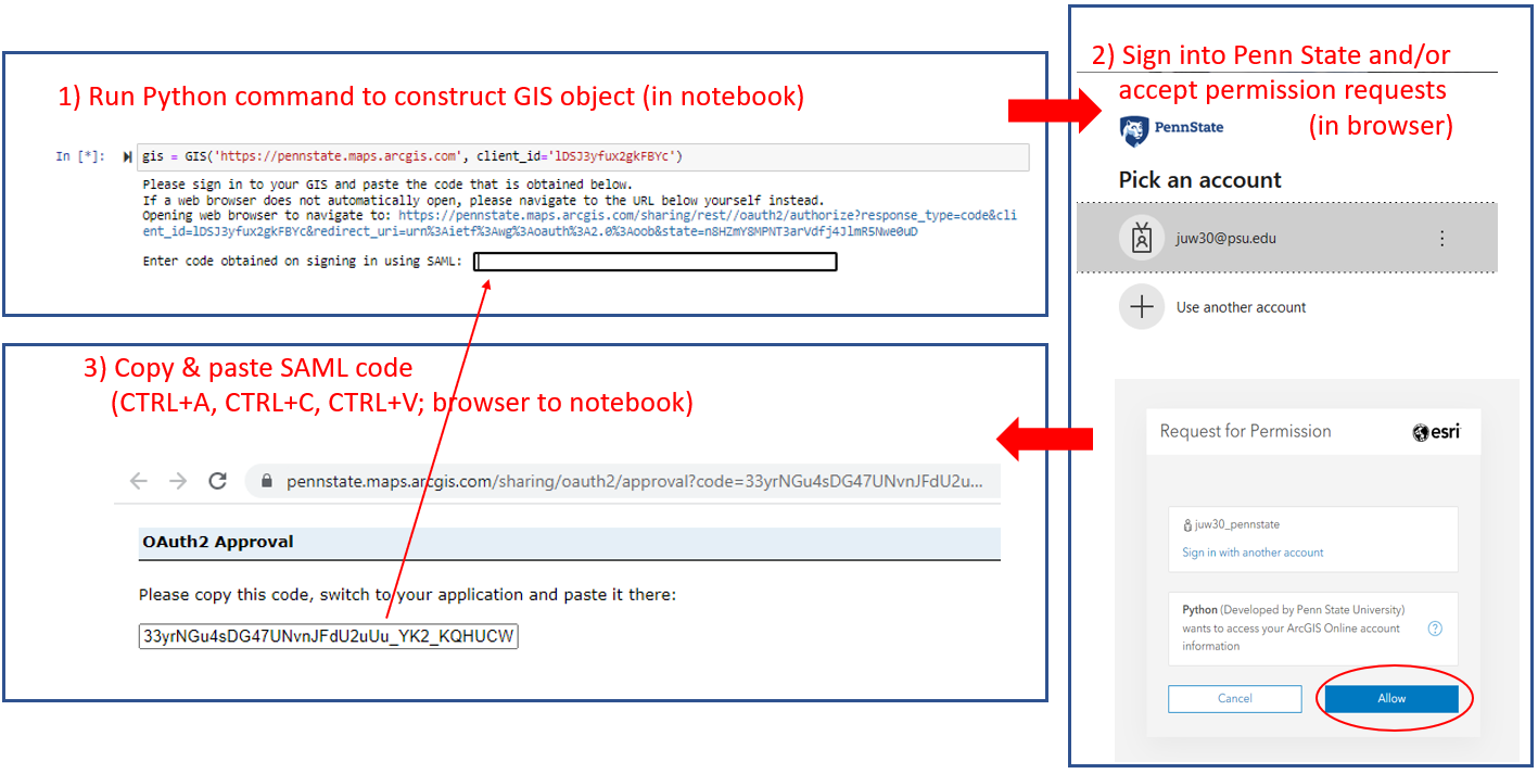
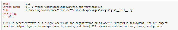
The GIS object in variable gis gives you access to a user manager (gis.users), a group manager (gis.groups) and a content manager (gis.content) object. The first two are useful for performing administrative tasks related to groups and user management. If you are interested in these topics, please check out the examples on the Accessing and Managing Users and Batch Creation of Groups pages. Here we simply use the get(...) method of the user manager to access information about a user, namely ourselves. Again, you will have to replace the <your username> tag with your PSU AGOL name to get some information display related to your account:
user = gis.users.get('<your username>')
user
The user object now stored in variable user contains much more information about the given user in addition to what is displayed as the output of the previous command. To see a list of available attributes, type in
user.
and then press the TAB key for the Jupyter autocompletion functionality. The following command prints out the email address associated with your account:
user.email
We will talk about the content manager object in a moment. But before that, let’s talk about maps and how easy it is to create a web map like visualization in a Jupyter Notebook with the ArcGIS API. A map can be created by calling the map(...) method of the GIS object. We can pass a string parameter to the method with the name of a place that should be shown on the map. The API will automatically try to geocode that name and then set up the parameters of the map to show the area around that place. Let’s use State College as an example:
map = gis.map('State College, PA')
map
The API contains a widget for maps so that these will appear as an interactive map in a Jupyter Notebook. As a result, you will be able to pan around and use the buttons at the top left to zoom the map. The map object has many properties and methods that can be used to access its parameters, affect the map display, provide additional interactivity, etc. For instance, the following command changes the zoom property to include a bit more area around State College. The map widget will automatically update accordingly.
map.zoom = 11
With the following command, we change the basemap tiles of our map to satellite imagery. Again the map widget automatically updates to reflect this change.
map.basemap = 'satellite'
As another example, let’s add two simple circle marker objects to the map, one for Walker Building on the PSU campus, the home of the Geography Department, and one for the Old Main building. The ArcGIS API provides a very handy geocode(...) function in the arcgis.geocoding module so that we won’t have to type in the coordinates of these buildings ourselves. The properties of the marker are defined in the pt_sym dictionary.
from arcgis.geocoding import geocode
pt_sym = {
"type": "esriSMS",
"style": "esriSMSCircle",
"color": [255,0,0,255],
}
walker = geocode('Walker Bldg, State College, PA')[0]
oldMain = geocode('Old Main Bldg, State College, PA')[0]
map.draw(walker, {'title':'Walker Bldg', 'content': walker['attributes']['LongLabel']}, symbol=pt_sym)
map.draw(oldMain, {'title':'Old Main Bldg', 'content': oldMain['attributes']['LongLabel']}, symbol=pt_sym)
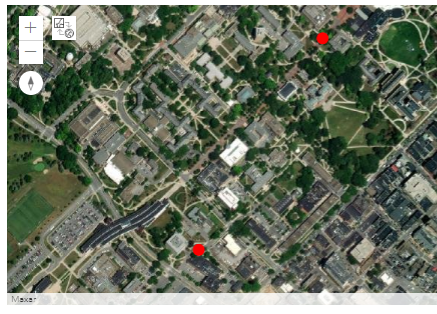
The map widget should now include the markers for the two buildings as shown in the image above (the markers may look different). A little explanation on what happens in the code: the geocode(...) function returns a list of candidate entities matching the given place name or address, with the candidate considered most likely appearing as the first one in the list. We here simply trust that the ArcGIS API has been able to determine the correct candidate and hence just take the first object from the respective lists via the “[0]” in the code. What we have now stored in variables walker and oldMain are dictionaries with many attributes to describe the entities. When adding the markers to the map, we provide the respective variables as the first parameter and the API will automatically access the location information in the dictionaries to figure out where the marker should be placed. The second parameter is a dictionary that specifies what should be shown in the popup that appears when you click on the marker. We use short names for the title of the popups and then use the ‘LongLabel’ property from the dictionaries, which contains the full address, for the content of the popups.
Let's have a look at a last map example demonstrating how one can use the API to manually draw a route from Walker building to Old Main and have the API calculate the length of that route. The first thing we do is import the lengths(...) function from the arcgis.geometry module and define a function that will be called once the route has been drawn to calculate the length of the resulting polyline object that is passed to the function in parameter g:
from arcgis.geometry import lengths
def calcLength(map,g):
length = lengths(g['spatialReference'], [g], "", "geodesic")
print('Length: '+ str(length[0]) + 'm.')
Once the length has been computed, the function will print out the result in meters. We now register this function as the function to be called when a drawing action on the map has terminated. In addition, we define the symbology for the drawing to be a dotted red line:
map.on_draw_end(calcLength)
line_sym = {
"type": "esriSLS",
"style": "esriSLSDot",
"color": [255,0,0,255],
"width": 3
}
With the next command we start the drawing with the ‘polyline’ tool. Before you execute the command, it's a good idea to make sure the map widget is zoomed in to show the area between the two markers but you will still be able to pan the map by dragging with the left mouse button pressed and to zoom with the mouse wheel during the drawing. You need to do short clicks with the left mouse button to set the points for the start point and end points of the line segments. To end the polyline, make a double click for the last point while making sure you don't move the mouse at the same time. After this, the calculated distance will appear under the map widget.
map.draw('polyline', symbol=line_sym)
You can always restart the drawing by executing the previous code line again. Using the command map.clear_graphics() allows for clearing all drawings from the map but you will have to recreate the markers after doing so.
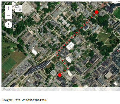
Now let’s get back to the content manager object of our GIS. The content manager object allows us to search and use all the content we have access to. That includes content we have uploaded and published ourselves but also content published within our organization and content that is completely public on AGOL. Content can be searched with the search(...) method of the content manager object. The method takes a query string as parameter and has additional parameters for setting the item type we are looking for and the maximum number of entries returned as a result for the query. For instance, try out the following command to get a list of available feature services that have PA in the title:
featureServicesPA = gis.content.search(query='title:PA', item_type='Feature Layer Collection', max_items = 50) featureServicesPA
This will display a list of different AGOL feature service items available to you. The list is probably rather short at the moment because not much has been published in the new pennstate organization yet, but there should at least be one entry with municipality polygons for PA. Each feature service from the returned list can, for instance, be added to your map or used for some spatial analysis. To add a feature service to your map as a new layer, you have to use the add_layer(...) method of the map object. For example, the following command takes the first feature service from our result list in variable featureServicesPA and adds it to our map widget:
map.add_layer(featureServicesPA[0], {'opacity': 0.8})
The first parameter specifies what should be added as a layer (the feature service with index 0 from our list in this case), while the second parameter is an optional dictionary with additional attributes (e.g., opacity, title, visibility, symbol, renderer) specifying how the layer should be symbolized and rendered. Feel free to try out a few other queries (e.g. using "*" for the query parameter to get a list of all available feature services) and adding a few other layers to the map by changing the index used in the previous command. If the map should get too cluttered, you can simply recreate the map widget with the map = gis.map(...) command from above.
The query string given to search(...) can contain other search criteria in addition to ‘title’. For instance, the following command lists all feature services that you are the owner of (replace <your agol username> with your actual Penn State AGOL/Pro user name):
gis.content.search(query='owner:<your agol username>', item_type='Feature Service')
Unless you have published feature services in your AGOL account, the list returned by this search will most likely be empty ([]). So how can we add new content to our GIS and publish it as a feature service? That’s what the add(...) method of the content manager object and the publish(...) method of content items are for. The following code uploads and publishes a shapefile of larger cities in the northeast of the United States.
To run it, you will need to first download the zipped shapefile and then slightly change the filename on your computer. Since AGOL organizations must have unique services names, edit the file name to something like ne_cities_[initials].zip or ne_cities_[your psu id].zip so the service name will be unique to the organization. Adapt the path used in the code below to refer to this .zip file on your disk.
neCities = gis.content.add({'type': 'Shapefile'}, r'C:\489\L3\ne_cities.zip')
neCitiesFS = neCities.publish()
The first parameter given to gis.content.add(...) is a dictionary that can be used to define properties of the data set that is being added, for instance tags, what type the data set is, etc. Variable neCitiesFS now refers to a published content item of type arcgis.gis.Item that we can add to a map with add_layer(...). There is a very slight chance that this layer will not load in the map. If this happens for you - continue and you should be able to do the buffer & intersection operations later in the walkthrough without issue. Let’s do this for a new map widget:
cityMap = gis.map('Pennsylvania')
cityMap.add_layer(neCitiesFS, {})
cityMap
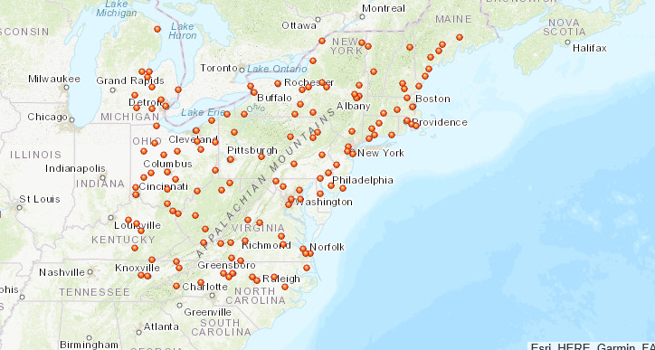
The image shows the new map widget that will now be visible in the notebook. If we rerun the query from above again...
gis.content.search(query='owner:<your agol username>', item_type='Feature Service')
...our newly published feature service should now show up in the result list as:
<Item title:"ne_cities" type:Feature Layer Collection owner:<your AGOL username>>
3.10.2 Accessing features and geoprocessing tools
The ArcGIS Python API also provides the functionality to access individual features in a feature layer, to manipulate layers, and to run analyses from a large collection of GIS tools including typical GIS geoprocessing tools. Most of this functionality is available in the different submodules of arcgis.features. To give you a few examples, let’s continue with the city feature service we still have in variable neCitiesFS from the previous section. A feature service can actually have several layers but, in this case, it only contains one layer with the point features for the cities. The following code example accesses this layer (neCitiesFE.layers[0]) and prints out the names of the attribute fields of the layer by looping through the ...properties.fields list of the layer:
for f in neCitiesFS.layers[0].properties.fields: print(f)
When you try this out, you should get a list of dictionaries, each describing a field of the layer in detail including name, type, and other information. For instance, this is the description of the STATEABB field:
{
"name": "STATEABB",
"type": "esriFieldTypeString",
"actualType": "nvarchar",
"alias": "STATEABB",
"sqlType": "sqlTypeNVarchar",
"length": 10,
"nullable": true,
"editable": true,
"domain": null,
"defaultValue": null
}
The query(...) method allows us to create a subset of the features in a layer using an SQL query string similar to what we use for selection by attribute in ArcGIS itself or with arcpy. The result is a feature set in ESRI terms. If you look at the output of the following command, you will see that this class stores a JSON representation of the features in the result set. Let’s use query(...) to create a feature set of all the cities that are located in Pennsylvania using the query string "STATEABB"='US-PA' for the where parameter of query(...):
paCities = neCitiesFS.layers[0].query(where='"STATEABB"=\'US-PA\'') print(paCities.features) paCities
Output:
[{"geometry": {"x": -8425181.625237303, "y": 5075313.651659228},
"attributes": {"FID": 50, "OBJECTID": "149", "UIDENT": 87507, "POPCLASS": 2, "NAME":
"Scranton", "CAPITAL": -1, "STATEABB": "US-PA", "COUNTRY": "USA"}}, {"geometry":
{"x": -8912583.489066456, "y": 5176670.443556941}, "attributes": {"FID": 53,
"OBJECTID": "156", "UIDENT": 88707, "POPCLASS": 3, "NAME": "Erie", "CAPITAL": -1,
"STATEABB": "US-PA", "COUNTRY": "USA"}}, ... ]
<FeatureSet> 10 features
Of course, the queries we can use with the query(...) function can be much more complex and logically connect different conditions. The attributes of the features in our result set are stored in a dictionary called attributes for each of the features. The following loop goes through the features in our result set and prints out their name (f.attributes['NAME']) and state (f.attributes['STATEABB']) to verify that we only have cities for Pennsylvania now:
for f in paCities: print(f.attributes['NAME'] + " - "+ f.attributes['STATEABB'])
Output: Scranton - US-PA Erie - US-PA Wilkes-Barre - US-PA ... Pittsburgh - US-PA
Now, to briefly illustrate some of the geoprocessing functions in the ArcGIS Python API, let’s look at the example of how one would determine the parts of the Appalachian Trail that are within 30 miles of a larger Pennsylvanian city. For this we first need to upload and publish another data set, namely one that’s representing the Appalachian Trail. We use a data set that we acquired from PASDA for this, and you can download the DCNR_apptrail file here. As with the cities layer earlier, there is a very small chance that this will not display for you - but you should be able to continue to perform the buffer and intersection operations. The following code uploads the file to AGOL (don’t forget to adapt the path and add your initials or ID to the name!), publishes it, and adds the resulting trail feature service to your cityMap from above:
appTrail = gis.content.add({'type': 'Shapefile'}, r'C:\489\L3\dcnr_apptrail_2003.zip')
appTrailFS = appTrail.publish()
cityMap.add_layer(appTrailFS, {})
Next, we create a 30 miles buffer around the cities in variable paCities that we can then intersect with the Appalachian Trail layer. The create_buffers(...) function that we will use for this is defined in the arcgis.features.use_proximity module together with other proximity based analysis functions. We provide the feature set we want to buffer as the first parameter, but, since the function cannot be applied to a feature set directly, we have to invoke the to_dict() method of the feature set first. The second parameter is a list of buffer distances allowing for creating multiple buffers at different distances. We only use one distance value, namely 30, here and also specify that the unit is supposed to be ‘Miles’. Finally, we add the resulting buffer feature set to the cityMap above.
from arcgis.features.use_proximity import create_buffers
bufferedCities = create_buffers(paCities.to_dict(), [30], units='Miles')
cityMap.add_layer(bufferedCities, {})
As the last step, we use the overlay_layers(...) function defined in the arcgis.features.manage_data module to create a new feature set by intersecting the buffers with the Appalachian Trail polylines. For this we have to provide the two input sets as parameters and specify that the overlay operation should be ‘Intersect’.
from arcgis.features.manage_data import overlay_layers trailPartsCloseToCity = overlay_layers(appTrailFS, bufferedCities, overlay_type='Intersect')
We show the result by creating a new map ...
resultMap = gis.map('Pennsylvania')
resultMap
... and just add the features from the resulting trailPartsCloseToCity feature set to this map:
resultMap.add_layer(trailPartsCloseToCity)
The result is shown in the figure below.
3.10.3 More examples and additional materials
This section gave you a brief introduction to ESRI's ArcGIS API for Python and showed you some of the most important methods and patterns that you will typically encounter when using the API. The API is much too rich to cover everything here, so, to get a better idea of the geoprocessing and other capabilities of the API, we recommend that you check and try out some of the sample notebooks that ESRI has published, such as:
A lot of valuable information can also be gained from the ESRI's API guide, and, of course, the API documentation.
3.11 Walkthrough: Species distribution modeling with Jupyter
You now have a basic understanding of the species distribution modeling task we want to solve in this lesson's walkthrough as well as the different Python packages that will play a role in preparing the data, running the model, and visualizing the result. Since all of this will take place within a Jupyter notebook, the remainder of this section will consist of the notebook itself exported to html and embedded into the Drupal pages for this lesson. Here is the link to the data you need for this walkthrough:
Link to L3 Walkthrough data, which you will need to download and extract to a new folder
Instead of just reading through the HTML version of the notebook content linked below, you should download the notebook, extract the contained .ipynb notebook file, place it in your user home or documents folder, open it with Jupyter and work through it step-by-step following the instructions given in the notebook itself, executing the code cells, and trying to understand the code sections and the output they produce.
Important note: Sections 3.1 and 5.2 of the notebook will use the Python-to-R interface (Section 3.7 of the lesson materials). On the R side, there are three packages involved: dismo, maptools, and rgdal.
While the environment we installed in Section 3.2 contains conda packages for dismo and maptools, there is at the moment no conda package available for rgdal because of technical issues the package maintainers have to resolve (see https://github.com/conda-forge/r-rgdal-feedstock/issues/18). We are therefore currently installing the rgdal package in the notebook code itself with the line "%R install.packages('rgdal')" close to the beginning. However, we in the past had a very few cases where this caused problems on some computers. Just in case you find yourself unable to run some of the R commands (starting with %R) in sections 3.1 and 5.2 of the notebook, we are here providing two files that can be used as a workaround. You will then have to place these files in your workspace folder for this walkthrough (just read the corresponding sections in the HTML export of the notebook linked below to see the output produced by the steps you cannot run yourself) and then follow the workaround instructions in the notebook that explain how to continue with the other sections with the help of these two files.
Here is the link to html export of the notebook if you want to have a look at it outside of Jupyter Notebook: HTML export of the walkthrough notebook
Reminder:
Complete all of the lesson tasks!
You have finished the Lesson 3 course materials. On the next pages, you will find a few practice exercises and the instructions for the Lesson 3 homework assignment. Double-check the list of requirements on the Lesson 3 Checklist page to make sure you have completed all of the activities listed there before beginning the next lesson.
3.12 Lesson 3 Practice Exercises
Again, we are going to close out the lesson with a few practice exercises that focus on the new Python concepts introduced in this lesson (regular expressions and higher order functions) as well as on working with tabular data with pandas as a preparation for this lesson's homework assignment. In the homework assignment, you are also going to use geopandas, the Esri ArcGIS for Python API, and GDAL/OGR again to get some more practice with these libraries, too. What was said in the introduction to the practice exercises of Lesson 2 holds here as well: don't worry if you have troubles finding the perfect solution on your own. Studying the solutions carefully is another way of learning and improving your skills. The solutions of the three practice exercises pages can again be found in the following subsections.
Practice Exercise 1: Regular Expressions (see Section 3.3)
Write a function that tests whether an entered string is a valid date using the format "YYYY-MM-DD". The function takes the string to test as a parameter and then returns True or False. The YYYY can be any 4-digit number, but the MM needs to be a valid 2-digit number for a month (with a leading 0 for January to September). The DD needs to be a number between 01 and 31 but you don’t have to check whether this is a valid number for the given month. Your function should use a single regular expression to solve this task.
Here are a few examples you can test your implementation with:
"1977-01-01" -> True "1977-00-01" -> False (00 not a valid month) "1977-23-01" -> False (23 not a valid month) "1977-12-31" -> True "1977-11-01asdf" -> False (you need to make sure there are no additional characters after the date) "asdf1977-11-01" -> False (you need to make sure there are no additional characters before the date) "9872-12-31" -> True "0000-12-33" -> False (33 is not a valid day) "0000-12-00" -> False (00 not a valid day) "9872-15-31" -> False (15 is not a valid month)
Practice Exercise 2: Higher Order Functions (see Section 3.4)
We mentioned that the higher-order function reduce(...) can be used to do things like testing whether all elements in a list of Booleans are True. This exercise has three parts:
- Given list l containing only Boolean values as elements (e.g. l = [ True, False, True ]), use reduce(…) to test whether all elements in l are True? What would you need to change to test if at least one element is True? (Hint: you will have to figure out what the right logical operator to use is and then look at how it’s called in the Python module operator; then figure out what the right initial value for the third parameter of reduce(...) is.)
- Now instead of a list of Booleans, you have a list of integer numbers (e.g. l =[-4, 2, 1, -6 ]). Use a combination of map(…) and reduce(…) to check whether or not all numbers in the list are positive numbers (> 0).
- Implement reduce(...) yourself and test it with the example from part 1. Your function myReduce(…) should have the three parameters f (function), l (list), and i (initial value). It should consist of a for-loop that goes through the elements of the list and it is not allowed to use any other higher order function (in particular not the actual reduce(...) function).
Practice Exercise 3: Pandas (see Section 3.8)
Below is an imaginary list of students and scores for three different assignments.
| Name | Assignment 1 | Assignment 2 | Assignment 3 | |
|---|---|---|---|---|
| 1 | Mike | 7 | 10 | 5.5 |
| 2 | Lisa | 6.5 | 9 | 8 |
| 3 | George | 4 | 3 | 7 |
| 4 | Maria | 7 | 9.5 | 4 |
| 5 | Frank | 5 | 5 | 5 |
Create a pandas data frame for this data (e.g. in a fresh Jupyter notebook). The column and row labels should be as in the table above.
Now, use pandas operations to add a new column to that data frame and assign it the average score over all assignments for each row.
Next, perform the following subsetting operations using pandas filtering with Boolean indexing:
- Get all students with an Assignment 1 score < 7 (show all columns)
- Get all students with Assignment 1 and Assignment 2 scores both > 6 (show all columns)
- Get all students with at least one score < 5 over all assignments (show all columns)
(Hint: an alternative to using the logical or (|) over all columns with scores is to call the .min(…) method of a data frame with the parameter "axis = 1" to get the minimum value over all columns for each row. This can be used here to first create a vector with the minimum score over all three assignments and then create a Boolean vector from it based on whether or not the value is <5. You can then use this vector for the Boolean indexing operation.)
- Get all students whose names start with 'M' and only show the name and average score columns
(Hint: there is also a method called .map(…) that you can use to apply a function or lambda expression to a pandas data frame (or individual column). The result is a new data frame with the results of applying the function/expression to each cell in the data frame. This can be used here to create a Boolean vector based on whether or not the name starts with ‘M’ (string method startswith(…)). This vector can then be used for the Boolean indexing operation. Then you just have to select the columns of interest with the last part of the statement).
- Finally, sort the table by name.
Lesson 3 Exercise 1 Solution
import re
datePattern = re.compile('\d\d\d\d-(0[1-9]|1[0-2])-(0[1-9]|[12]\d|3[01])$')
def isValidDate(s):
return datePattern.match(s) != None
Explanation: Since we are using match(…) to compare the compiled pattern in variable datePattern to the string in parameter s given to our function isValidDate(…), we don’t have to worry about additional characters before the start of the date because match(…) will always try to match the pattern to the start of the string. However, we use $ as the last character in our pattern to make sure there are no additional characters following the date. That means the pattern has the form
“…-…-…$”
where the dots have to be replaced with some regular expression notation for the year, month, and day parts. The year part is easy, since we allow for any 4-digit number here. So we can use \d\d\d\d here, or alternatively \d{4,4} (remember that \d stands for the predefined class of all digits).
For the month, we need to distinguish two cases: either it is a 0 followed by one of the digits 1-9 (but not another 0) or a 1 followed by one of the digits 0-2. We therefore write this part as a case distinction (…|…) with the left part 0[1-9] representing the first option and the second part 1[0-2] representing the second option.
For the day, we need to distinguish three cases: (1) a 0 followed by one of the digits 1-9, (2) a 1 or 2 followed by any digit, or (3) a 3 followed by a 0 or a 1. Therefore we use a case-distinction with three options (…|…|…) for this part. The first part 0[1-9] is for option (1), the second part [12]\d for option (2), and the third part 3[01] for the third option.
Lesson 3 Exercise 2 Solution
Part 1:
import operator from functools import reduce l = [True, False, True] r = reduce(operator.and_, l, True) print(r) # output will be False in this case
To check whether or not at least one element is True, the call has to be changed to:
r = reduce(operator.or_, l, False)
Part 2:
import operator from functools import reduce l = [-4, 2, 1, -6 ] r = reduce(operator.and_, map(lambda n: n > 0, l), True) print(r) # will print False in this case
We use map(…) with a lambda expression for checking whether or not an individual element from the list is >0. Then we apply the reduce(…) version from part 1 to the resulting list of Boolean values we get from map(…) to check whether or not all elements are True.
Part 3:
import operator l = [True, False, True] def myReduce(f, l, i): intermediateResult = i for element in l: intermediateResult = f(intermediateResult, element) return intermediateResult r = myReduce(operator.and_, l, True) print(r) # output will be False in this case
Maybe you were expecting that an implementation of reduce would be more complicated, but it’s actually quite simple. We set up a variable to always contain the intermediate result while working through the elements in the list and initialize it with the initial value provided in the third parameter i. When looping through the elements, we always apply the function given in parameter f to the intermediate result and the element itself and update the intermediate result variable with the result of this operation. At the end, we return the value of this variable as the result of the entire reduce operation.
Lesson 3 Exercise 3 Solution
import pandas as pd
# create the data frame from a list of tuples
data = pd.DataFrame( [('Mike',7,10,5.5),
('Lisa', 6.5, 9, 8),
('George', 4, 3, 7),
('Maria', 7, 9.5, 4),
('Frank', 5, 5, 5) ] )
# set column names
data.columns = ['Name', 'Assignment 1', 'Assignment 2', 'Assignment 3']
# set row names
data.index = range(1,len(data)+1)
# show table
print(data)
# add column with averages
data['Average'] = (data['Assignment 1'] + data['Assignment 2'] + data['Assignment 3']) / 3
# part a (all students with a1 score < 7)
print(data[ data['Assignment 1'] < 7])
# part b (all students with a1 and a2 score > 6)
print(data[ (data['Assignment 1'] > 6) & (data['Assignment 2'] > 6)])
# part c (at least one assignment < 5)
print( data[ data[ ['Assignment 1', 'Assignment 2', 'Assignment 3'] ].min(axis = 1) < 5 ] )
# part d (name starts with M, only Name and Average columns)
print(data [ data [ 'Name' ].map(lambda x: x.startswith('M')) ] [ ['Name','Average'] ])
# sort by Name
print(data.sort_values(by = ['Name']))
If any of these steps is unclear to you, please ask for further explanation on the forums.
3.13 Lesson 3 Assignment
In this homework assignment, we want you to practice working with pandas and the other Python packages introduced in this lesson some more, and you are supposed to submit your solution as a nice-looking Jupyter Notebook including well-formatted explanations of each step. While the assignment could be solved using pandas, geopandas, and the Esri Python API alone, we are asking you to use GDAL/OGR for one of the steps involved so that you get some further practice with that library as well. To solve the task, you will occasionally have to use the packages in ways that we did not show in the lesson materials. In addition, you will have to work with the Python datetime module for representing dates & times in Python code. That means you will also have to practice working with the respective documentations and complementing web resources a bit. However, we did include some pointers in the instructions below, so that you have an idea of where to look, and also provided some examples.
The situation is the following: You have been hired by a company active in the northeast of the United States to analyze and produce different forms of summaries for the traveling activities of their traveling salespersons. Unfortunately, the way the company has been keeping track of the related information leaves a lot to be desired. The information is spread out over numerous .csv files. Please download the .zip file containing all (imaginary) data you need for this assignment and extract it to a new folder. Then open the files in a text editor and read the explanations below.
Explanation of the files:
File employees.csv: Most data files of the company do not use the names of their salespersons directly but instead refer to them through an employee ID. This file maps employee name to employee ID number. It has two columns, the first contains the full names in the format first name, last name and the second contains the ID number. The double quotes around the names are needed in the csv file to signal that this is the content of a single cell containing a comma rather than two cells separated by a comma.
"Smith, Richard",1234421 "Moore, Lisa",1231233 "Jones, Frank",2132222 "Brown, Justine",2132225 "Samulson, Roger",3981232 "Madison, Margaret",1876541
Files travel_???.csv: each of these files describes a single trip by a salesperson. The number in the file name is not the employee ID but a trip number. There are 75 such files with numbers from 1001 to 1075. Each file contains just a single row; here is the content of one of the files, the one named travel_1001.csv:
2132222,2016-01-07 16:00:00,2016-01-26 12:00:00,Cleveland;Bangor;Erie;Philadelphia;New York;Albany;Cleveland;Syracuse
The four columns (separated by comma) have the following content:
- the ID of the employee who did this trip (here: 2132222),
- the start date and time of the trip (here: 2016-01-07 16:00:00),
- the end date and time of the trip (here: 2016-01-26 12:00:00),
- and the route consisting of the names of the cities visited on the trip as a string separated by semi-colons (here: Cleveland;Bangor;Erie;Philadelphia;New York;Albany;Cleveland;Syracuse). Please note that the entire list of cities visited is just a single column in the csv file!
File ne_cities.shp: You already know this shapefile from the lesson content. It contains larger cities in the northeast U.S.A. as WGS84 points. The only attribute relevant for this exercise in addition to the point geometry is the NAME field containing the city names.
There are a few more files in the folder. They are actually empty but you are not allowed to delete these from the folder. This is to make sure that you have to be as specific as possible when using regular expressions for file names in your solution.
Your Task
The Python code you are supposed to write should take three things as input:
- a list of employee names (e.g., ['Jones, Frank', 'Brown, Justine', 'Samulson, Roger'] ),
- a start date (e.g., '2016-06-26'),
- and an end date as input (e.g., '2017-05-11').
It should then produce two output files:
- A new .csv file that lists the trips made by employees from the given employee name list that took place between the given start and end dates with all information from the respective travel_???.csv files as well as the name of the employee and the duration of each trip in days. The rows should be ordered by employee name -> trip duration -> start date -> end date. The figure below shows the exemplary content of this output file.
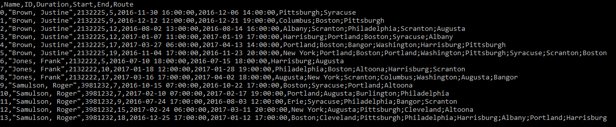 Example CSV Output File
 - A WGS1984 shapefile that shows the individual trips from the csv file created in (1) as polyline features. The attributes of the shapefile should be the name of the employee, the city list as a single string attribute, and the duration only. You will also have to zip this shapefile and upload & publish it as a feature service on ArcGIS Online.
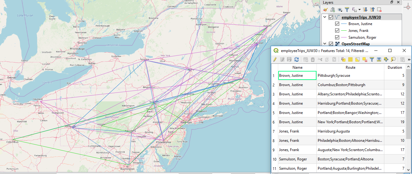 Example Output Shapefile Shown in QGIS
You should develop your solution as a Jupyter notebook with nicely formatted explanations of each step in your solution, similar to the L3 walkthrough notebook. Your notebook should at the end contain a map widget from the Esri Python API that displays the polyline feature service as a layer (similar to the lesson walkthrough notebook). You will submit this notebook file together with your write-up to the L3 assignment drop box on Canvas. The two images above have been produced using the example input values we gave above, so the name list 'Jones, Frank', 'Brown, Justine', and 'Samulson, Roger', the start date 2016-06-26, and the end date 2017-05-11. You can use this example for testing your solution.
Preparation
The assignment will require you to work with objects of the classes datetime and timedelta defined in the module datetime of the Python standard library to represent time stamps (combinations of date & time) and differences between them. The official documentation for the module is available at this Python documentation page. In addition, you can find two links to introductions to datetime below that may be a bit easier to digest. Please check these out and make sure you understand how to work with the datetime class, how to compare datetime objects to see whether one is earlier than the other and how to calculate a timedelta object for the difference between two datetime objects. Time zones won’t matter in this assignment.
- Python DateTime, TimeDelta, Strftime (Format) with Examples
- Working with datetime objects and timezones in Python
Below are a few examples illustrating how to create datetime objects representing concrete dates, how to calculate the time difference (datetime object timedelta) between two datetime objects, and how to compare two datetime objects using the < or > operators. These examples should be easy to understand, in particular when you have read through the documentation linked above. If you have any remaining questions on using datetime, please ask them on the course forums.
import datetime # create datetime objects for specific dates date1 = datetime.datetime(2019, 1, 31, 17, 55) # create datetime object for January 31, 2019, 17:55pm date2 = datetime.datetime(2019, 3, 12, 0, 0) # create datetime object for March 12, 2019, 0am print(date1) print(type(date1)) print(date2)Output:
2019-01-31 17:55:00 <class 'datetime.datetime'> 2019-03-12 00:00:00
# calculate the time difference between two datetime objects delta = date2 - date1 print(delta) print(type(delta)) print(delta.days) # difference in days print(delta.seconds) # difference in secondsOutput:
39 days, 6:05:00 <class 'datetime.timedelta'> 39 21900
# comparing datetime objects
if (date2 < date1):
print('before')
else:
print('after')
Output:
after
Steps in Detail:
Your notebook should roughly follow the steps below; in particular you should use the APIs mentioned for performing each of the steps:
- The input variables defined at the beginning of your notebook should include
- the list of employee names to include in the output
- the start date and end dates as datetime.datetime objects
- the folder that contains the input files
- the name of the output shapefile (include your initials or ID in the name to make the name unique for uploading it to AGOL)
- the name of the output csv file
- Use pandas (Section 3.8) to read the data from employees.csv into a data frame (see Hint 1).
- Use pandas to create a single data frame with the content from all 75 travel_???.csv files. The content from each file should form a row in the new data frame. The dates should be represented as datetime objects in the data frame (see Hints 1 and 2). Use regular expression and the functions from the re package for this step (Section 3.3) to only include files that start with "travel_", followed by a number, and ending in ".csv".
- Use pandas operations to join (see Section 3.8.5) the two data frames from steps (2) and (3) using the employee ID as key. Derive from this combined data frame a new data frame with
- only those rows that contain trips of employees from the input name list and with a start date after the given start date and an end date before the given end date (see Hint 3)
- an additional column that contains the duration of the trips in days (computed by subtracting start from end date)
- columns appearing in the order “Name”, “ID”, “Duration”, “Start”, “End”, and “Route” with these labels, and row labels being integer numbers 0,1,2,… (see image of example csv output file above)
- rows sorted by employees' names as the first criterion, followed by duration (meaning all trips for the same person are ordered from shortest to longest), start date, and end date as criteria.
- Write the data frame produced in the previous step to a new csv file using the specified output file name from (1) (see Hint 1 and image of example csv output file above).
- Use geopandas (Section 6.1 of the Juypter notebook from the lesson walkthrough) and its read_file(...) function to read the ne_cities.shp shapefile into a data frame. Reading a shapefile with the read_file(...) geopandas function is straightforward and you shouldn’t have any trouble finding some examples on the web. The result is a special geopandas data frame object that has a column called geometry which contains Shapely Point objects with WGS84 coordinates for the cities.
- Use GDAL/OGR (Section 3.9) to create a new shapefile with polyline features for each trip in the combined data frame from step (5) and attributes “Name” with the employee's name, “Route” with the city list for that trip, and “Duration” in days (see image of example output shapefile above). The polyline features need to be created from the city lists in the Route column and the point coordinates available in the geometry column of the ne_cities geopandas data frame produced in the previous step.
To create the new shapefile and populate it with features you can follow the general steps from creating the centroid buffer file in the last part of Section 3.9.1. The most tricky part will be to translate each trip into a WKT LineString that you then can create an OGR polyline feature from using the ogr.CreateGeometryFromWkt(...) function replacing the centroid and buffering part in the example from 3.9.1. Hint 4 shows how all the WKT LineStrings can be created to then be added as a new column to the combined data frame from step (5). This is done all in a single line with nested list comprehensions. If you feel very confident in your Python skills, you can try to write this code yourself (it doesn't necessarily have to be just a single line of code), else we recommend that you just use the code provided in the hint to do the translation. - Zip the shapefile produced in the previous step, then upload and publish it as a feature service on ArcGIS Online with the Esri API and include a map widget in your notebook showing the feature service as a layer (see Section 3.10 and the lesson walkthrough). You are allowed to reuse the code from the lesson walkthrough for this including the zipfile(...) function. Make sure that the name of the uploaded file is unique by incorporating your initials or ID).
Hint 1:
Pandas provides functions for reading and writing csv files (and quite a few other file formats). They are called read_csv(...) and to_csv(...). See this Pandas documentation site for more information and also the Python datetime documentation for datetime parsing specifics. When your input file contains dates that you want to become datetime objects, you should use the parse_dates and date_parser keyword arguments of read_csv(…) to let the method know which columns contain dates and how to interpret them (see the subsection on "Date Handling" on the page linked above). Here is an example of how this kind of command needs to look. The None for the header argument signals that the table in the csv file does not contain column names as the first row. The [...] for the parse_dates argument needs to be replaced by a list of column indices for the columns that contain dates in the csv file. The lambda function for the date_parser argument maps a date string we find in the input .csv file to a datetime object.
import pandas as pd import datetime df = pd.read_csv(r'C:\489\test.csv', sep=",", header=None, parse_dates=[...], date_parser= lambda x: datetime.datetime.strptime(x, '%Y-%m-%d %H:%M:%S'))
Hint 2:
The pandas concat(…) function can be used to combine several data frames with the same columns stored in a list to form a single data frame. This can be a good approach for this step. Let's say you have the individual data frames stored in a list variable called dataframes. You'd then simply call concat like this:
combinedDataFrame = pd.concat(dataframes)
This means your main task will be to create the list of pandas data frames, one for each travel_???.csv file before calling concat(...). For this, you will first need to use a regular expression to filter the list of all files in the input folder you get from calling os.listdir(inputFolder) to only the travel_???.csv files and then use read_csv(...) as described under Hint 1 to create a pandas DataFrame object from the csv file and add this to the data frame list.
Hint 3:
You can compare a datetime object (e.g. the start or end date) to a datetime column in a pandas data frame resulting in a Boolean vector that tells you whether the comparison is true or not for each row. Furthermore, you can use the pandas method isin(…) to check whether the string in the cells of a data frame or single column are contained in a given list of strings. The result is again a Boolean data frame/column. Together this allows you to select the desired rows via Boolean indexing as shown in Section 3.8.6. Here is a simple example showing how isin(...) is used to create a Boolean vector based on whether or not the name of each row is from a given list of names:
import pandas as pd names = ['Frank', 'James', 'Jane', 'Stevie'] # names we are interested in df = pd.DataFrame([['Martin', 5], # simple data frame with two columns ['James', 3], ['Sue', 1], ['Mark', 11], ['Stevie',3 ]] , columns=['Name', 'Grade']) booleanVector = df.Name.isin(names) print(booleanVector)
Output:
0 False 1 True 2 False 3 False 4 True Name: Name, dtype: bool
Hint 4:
The GDAL cookbook contains several examples of creating a polyline geometry from a WKT LineString that should be helpful to implement this step. In principle, the entire translation of the semi-colon-separated city list into a WKT LineString can be done with the following expression using two nested list comprehensions, but it is also ok if you break this down into several steps.
wkt = [ 'LineString (' + ','.join([ '{0} {1}'.format(cities[cities.NAME == city].geometry.x.iloc[0], cities[cities.NAME == city].geometry.y.iloc[0]) for city in r.split(';') ])+')' for r in fullInfoSorted.Route]
This code assumes that the geopandas data frame with the city data is stored in variable cities and that the combined trip data from step (5) is stored in variable fullInfoSorted such that fullInfoSorted.Route refers to the column with the route information consisting of city names separated by semicolons. In the outer list comprehension, we have variable r go through the cells (= rows) in the Route column. In the inner list comprehension
[ '{0} {1}'.format(cities[cities.NAME == city].geometry.x.iloc[0], cities[cities.NAME == city].geometry.y.iloc[0]) for city in r.split(';') ]
we then split the cell content at all semicolons with r.split(';') and have variable city go through all the cities in the given route. With the expression cities[cities.Name == city] we get the row for the given city from the cities data frame and, by appending .geometry.x.iloc[0] or .geometry.y.iloc[0], we get the corresponding x and y coordinates from the content of the geometry column of that row. The result of this inner list comprehension is a list of strings in which the x and y coordinates for each city are separated by a space, e.g. ['cx1 cy1', 'cx2 cy2', ... 'cxn cyx'] where cxi / cyi stands for the x/y coordinate of the i-th city in the trip. By using 'LineString (' + ','.join(...) + ')' in the outer list comprehension, we turn this list into a single string separated by comma, so 'cx1 cy1,cx2 cy2,...,cxn cyx' and add the prefix "LineString (" at the beginning and the closing ")" at the end producing the WKT string expression "LineString (cx1 cy1,cx2 cy2,...,cxn cyx)" for each trip. The resulting list of WKT LineStrings in variable wkt can now be added as a new column to the fullInfoSorted data frame as a basis for creating the GDAL features for the new shapefile by using ogr.CreateGeometryFromWkt(...) for each individual WKT LineString.
Grading Criteria
The criteria your notebook submission will be graded on will include how elegant and efficient your code is (e.g. try to make use of regular expressions and use list comprehension instead of for-loops where a simple list comprehension is sufficient) and how well your notebook documents and describes your solution in a visually appealing way.
Successful completion of the above requirements and the write-up discussed below is sufficient to earn 90% of the credit on this project. The remaining 10% is reserved for "over and above" efforts which could include, but are not limited to, the following:
- increase the flexibility of the notebook (e.g. allow for specifying a minimum and maximum duration for the trips that should be included),
- extend your solution to perform other analyses of the data (e.g. compute some statistics) using pandas as much as possible and writing the results to suitable output files,
- use GDAL or the ESRI Python API to incorporate some GIS analysis of the data or produce shapefiles that show the data in a different way (e.g. all cities visited by each of the employees from the list as individual point shapefiles).
Write-up
Produce a 400-word write-up on how the assignment went for you; reflect on and briefly discuss the issues and challenges you encountered and what you learned from the assignment. Please also briefly mention what you did for "over and above" points in the write-up.
Deliverable
Submit a single .zip file to the corresponding drop box on Canvas; the zip file should contain:
- Your Jupyter notebook file
- Your 400-word write-up
Final Project Proposal Assignment
At some point during this course, you've hopefully felt "the lightbulb go on" regarding how you might apply the lesson material to your own tasks in the GIS workplace. To conclude this course, just as we did in Geog 485, you will be expected to complete an individual project that uses Python automation to make some GIS task easier, faster, or more accurate.
The project goal is up to you, but it is preferably one that relates to your current field of work or a field in which you have a personal interest. We don't mind what packages or libraries you use – it can be an arcpy project, a Jupyter notebook, a QGIS program or plugin (to be discussed in Lesson 4), a standalone program, or some combination of the above.
What we are expecting is that you will use the advanced concepts that you have learned in the class where appropriate, so perhaps that means using list comprehension or multiprocessing or regular expressions (or all of them) depending on the problem that you're trying to solve. Feel free to use any of the packages that we've used already in the class (PyQt5, pandas, GDAL, etc.) or any others that interest you.
Since you're defining the requirements from the beginning, there is no "over and above" credit factored into this project grade. The number of lines of code you write is not as important as the problem you solve. However, we ask you to propose a project that meets or even slightly exceeds your relative level of experience with programming and that is significantly more complex than what you did as a term project for Geog 485.
You will have two weeks at the end of the term to dedicate completely toward the project. This is your chance to apply what you've learned about Advanced Python to a problem that really interests you. As with Geog 485, if you're implementing a solution for a work problem – that's fine – feel free to use synthetic (made up) data if that's necessary to ensure confidentiality.
One week into Lesson 4 you are required to submit a project proposal to the Final Project Proposal Drop Box in Canvas. This proposal must clearly explain:
- The task you intend to accomplish using Python
- How your proposed solution will make the task easier, faster, and/or more accurate. Also explain why your task could not simply be accomplished using the "out-of-the-box" tools from Esri, QGIS etc., or why your script gives a particular advantage over those tools
- What kind of tool this will be (arcpy script, Jupyter notebook, QGIS plugin, standalone Python program, …) and why you have decided to take this approach, as well as what other packages/libraries you expect to use for the project
- The deliverables you will submit for the project. Well-documented code is expected. If the script/tool/application requires data, describe how the instructors will be able to evaluate your script. Possible solutions are to zip a sample dataset for the instructors, demonstrate your script during a recorded video, or make the script flexible enough that it could be used with any dataset
The proposal will contribute toward 10% of your Final Project grade so please put some effort in describing your idea as clearly and in as much detail as possible. The proposal will also be used to help grade the rest of your project. Your proposal must be approved by the instructors before you move forward with coding the project. We may also offer some guidance on how to approach your particular task, and we'll provide thoughts on whether you are taking on too much or too little work to be successful.
As you work on your project, you're encouraged to seek help from all resources discussed in this class, including existing code samples and scripts on the Internet. If you re-use any sections of code that you found on the Internet, please thoroughly explain in your project writeup how you found it, tested it, and extracted only the parts you needed.
You will be graded based on the level of difficulty of your project, relative to your skills, the quality of the code, documentation and writeup, whether or not the code solves the problem you defined, and the elegance of your solution (is it efficient and well crafted; there are some tips on how to write elegant code here - Writing Elegant and Readable Code).
Project Ideas
If you're having trouble thinking up a project, you can derive a proposal from one of the suggestions here which are broadly the same as in Geog 485. But now we expect that you'll extend and expand on them significantly using what you know about various packages, libraries and delivery methods (Jupyter Notebooks, QGIS plugins and building your own GUI tools). So please see these only as core ideas to develop a project around, not as complete task specifications for a project.
You may have to spend a little bit of time acquiring or making up some test datasets to fit these project ideas. I also suggest that you read through the Lesson 4 material before selecting a project, just so you have a better idea of what types of things are possible with Python.
- Compare dataset statistics: Make a tool or script that takes two feature classes or other datasets as input, along with field names. The tool should check whether or not the field data is the same in both data sources and exists in both feature classes. If both these conditions are met, the tool should calculate statistics for that field for both feature classes and report the difference. Statistics could be sum, average, standard deviation, etc. and produce an output file.
- Compare existence of features in two datasets: Make a tool or script that reads two feature classes based on a key field (such as OBJECTID). The tool should figure out which features only appear in one of the feature classes and write them to a third feature class. As a variation on this, the tool could figure out which features appear in both feature classes and write them to a third feature class. You should allow the tool user to set a parameter to determine this – perhaps even with a custom interface.
- Calculate and compare areas: Make a tool or script that tallies the areas of all geometries in a feature class, or subsets of geometries based on a query and reports the difference. For example, this tool might compare "Acres of privately owned wetlands in 2008" and "Acres of privately owned wetlands in 2009." Make your tool available in a number of locations or accessible in a number of ways (e.g. as an arcpy / ArcGIS script, QGIS plugin and on github as well).
- Find and replace: Make a tool flexible enough to search for any term in any field in a feature class and replace it with another user-provided term. Ensure in your code that users cannot modify the critical fields' OBJECTIDs or SHAPEs. Also ensure that partial strings are supported, such that if the search term is found anywhere within a string, it will be replaced while leaving the rest of the string intact.
- Process rasters to meet an organizational need: Write a tool or script that takes a raw elevation dataset (such as a DEM), clips it to your study area, creates both hillshade and slope rasters, and projects them into your organization's most commonly used projection. Expose the study area feature class to the end user as a parameter and perhaps perform all of this analysis in a Jupyter notebook and display the results.
- Parse raw textual data and write to feature class: Find some data available on the Internet that has lat/lon locations but is in text-based format with no Esri feature class available (for example, weather station readings or GPS tracks). If you need to, you can copy the HTML out of the Web page and paste it in a .txt file to help you get started. Read the .txt file and write the data to a new feature class. We've covered this in the lesson so you'll really need to extend this idea to make it interesting.
- Do a performance comparison between arcpy and gdal tools (for example) or numpy arrays and R code to perform comparable tasks (e.g. calculating slope / aspect for a raster) or updating values in a shapefile / table.
- Map data using arcpy mapping and incorporate plotly graphs of statistics into the map book with custom layouts, color schema or graphs depending on the type of analysis a user specifies (either from an Arc toolbox or via a pyqt5 interface).
Lesson 4 Object-Oriented Programming in Python and QGIS Development
4.1 Overview and Checklist
This lesson is two weeks in length. The focus will be on diving into the object-oriented programming aspects of Python and you will finally learn how to define your own classes in Python as well as derive new classes as subclasses of already existing classes. We will also return to the topic of GUI development and apply what we learned on object-oriented programming to create a standalone application and (optionally) plugin for the open-source GIS software QGIS. To prepare for that, the lesson starts with a theoretical section on Python collections, followed by an introduction to QGIS and its Python API.
After the end of the first week, you are supposed to submit a proposal for a term project. Please refer to the Calendar for specific time frames and due dates. To finish this lesson, you must complete the activities listed below. You may find it useful to print this page first so that you can follow along with the directions.
| Step | Activity | Access/Directions |
|---|---|---|
| 1 | Engage with Lesson 4 Content | Begin with 4.2 Collections and Sorting |
| 2 | Term project proposal | Submit your term project proposal by the end of the first week of the lesson |
| 3 | Programming Assignment and Reflection |
Submit your code for the programming assignment and 400 words write-up with reflections |
| 4 | Quiz 4 | Complete the Lesson 4 Quiz |
| 5 | Questions/Comments | Remember to visit the Lesson 4 Discussion Forum to post/answer any questions or comments pertaining to Lesson 4 |
4.2 Collections and Sorting
In programming, you are often dealing with collections of items of the same data type, e.g. collections of integer numbers, collections of Point objects, etc. You are already familiar with the built-in collection types list, tuple, and dictionary, but there exist more data structures for storing collections of items. Which data structure is best suited for a specific task depends on what operations exactly you need to perform with the data structure and items in it. For instance, a dictionary is the right choice if you mainly need to access the stored items based on their key. In contrast, a list is a good choice if you have a static collection of items that you need to iterate over or that you want to access based on their index. In general, there often exist several collection data types that you can use for a given task but some of them will be more efficient and better choices than the others.
Here is a little introductory example:
Let’s say that, in your Python program, you have different assignments or jobs coming in that need to be performed in the order in which they arrive. Since performing an assignment can take some time, you need to store the assignments in some sort of waiting queue: the next assignment to be performed is always taken from the front of the queue, while the new assignments arriving are added at the end of the queue. This approach is often referred to as the first-in-first-out (FIFO) approach.
To implement the waiting queue in this program, we could use a normal list. New assignments are added to the end of the list with list method append(), while items can be removed at the beginning of the list by calling the list method pop(...) with parameter 0. The following code simulates the arriving of new assignments and removing of the next assignment to be performed, starting with a queue with three assignments in it. For simplicity we alternate between an assignment being removed and a new assignment arriving, meaning the queue will always contain two or three assignments. We also simply use strings with an increasing number at the end for the assignments, while in a real application these would be more complex objects with attributes describing the assignment.
waitingQueue = ["Assignment 1", "Assignment 2", "Assignment 3"]
for count in range(3,100001):
waitingQueue.pop(0) # remove assignment at the beginning of the list/queue
waitingQueue.append("Assignment " + str(count)) # add new assignment at the end of the list/queue
Run this program with basic code profiling as explained in Section 1.7.2.1. One thing you should see in the profiling results is that while the Python list implementation is able to perform append operations (adding at the end of the list) rather efficiently, it is not particularly well suited for removing (and also adding) elements at the beginning. There exist data structures that are much better suited for this task as the following version shows. It uses the collection class deque (standing for “double-ended queue”) that is defined in the collections module of the Python standard library, which contains several specialized collection data structures. Deque is optimized for adding and removing elements at the start and end of the collection.
import collections
waitingQueue = collections.deque(["Assignment 1", "Assignment 2", "Assignment 3"])
for count in range(3,100001):
waitingQueue.popleft() # remove assignment at the beginning of the deque
waitingQueue.append("Assignment " + str(count)) # add new assignment at the end of the deque
Please note that the deque method for removing the first element from the queue is called popleft(), while pop() removes the last element. The method append() adds an element at the end, while appendleft() adds an element at the start (we don’t need pop() and appendleft() in this example). The initial deque is created by giving the list of three assignments as a parameter to collections.deque(...).
If you profile this second version and compare the results with those of the first version using a list, you should see that deque is by far the better choice for implementing this kind of waiting queue. More precisely, adding elements at the end takes about the same time as for lists but removing elements at the front is approximately three times as fast (and as fast as adding at the end).
While we cannot go into the implementation details of lists and deque here (you may want to check out a book on algorithms and data structures in Python to learn how to implement such collections yourself), hopefully this example makes it clear that it’s a good idea to have some understanding of what collection data structure are available and which operations are fast with them and which are slow.
In the following, we are going to take a quick look at sets and priority queues (or heaps) as two examples of other specialized Python collections, and we talk about the common operation of sorting collections.
4.2.1 Sets
Sets are another built-in collection in Python in addition to lists, tuples, and dictionaries. The idea is that of a mathematical set, meaning that there is no order between the elements and an element can only be contained in a set once (in contrast to lists). Sets are mutable like lists or dictionaries.
The following code example shows how we can create a set using curly brackets {…} to delimit the elements (similar to a dictionary but without the
s = {3,4,1,3,4,1} # create set
print(s)
Output:
{1, 3, 4}
Since sets are unordered, it is not possible to access their elements via an index but we can use the “in” operator to test whether or not a set contains an element as well as use a for-loop to iterate through the elements:
x = 3
if x in s:
print("already contained")
for e in s:
print(e)
Output: already contained 1 3 4
One of the nice things about sets is that they provide the standard set theoretical operations union, intersection, etc. as shown in the following code example:
group1 = { "Jim", "Maria", "Frank", "Susan"}
group2 = { "Sam", "Steve", "Jim" }
print( group1 | group2 ) # or group1.union(group2)
print( group1 & group2 ) # or group1.intersection(group2)
print( group1 - group2 ) # or group1.difference(group2)
print( group1 ^ group2 ) # or group1.symmetric_difference(group2)
Output:
{'Frank', 'Sam', 'Steve', 'Susan', 'Maria', 'Jim'}
{'Jim'}
{'Susan', 'Frank', 'Maria'}
{'Frank', 'Sam', 'Steve', 'Susan', 'Maria'}
The difference between the last and second-to-last operation here is that group1 - group2 returns the elements of the set in group1 that are not also elements of group2, while the symmetric difference operation group1 ^ group2 returns a set with all elements that are only contained in one of the groups but not in both.
4.2.2 Sorting
One common operation on collections is sorting the elements in a collection. Python provides a function sorted(…) to sort the elements in a collection that allows for iterating over the elements (e.g. a list, tuple, or dictionary). The result is always a list. Here are two examples:
l1 = [9,3,5,1,-2]
print(sorted(l1))
l2 = ("Maria", "Frank", "Sam", "Mike")
print(sorted(l2))
Output: [-2, 1, 3, 6, 9] ['Frank', 'Maria', 'Mike', 'Sam']
If our collection is a list, we can also use the list method sort() instead of the function sorted(…), e.g. l1.sort() instead of sorted(l1) . Both work exactly the same.
sorted(…) and sort() by default sort the elements in ascending order based on the < comparison operator. This means numbers are sorted in increasing order and strings are sorted in lexicographical order. When we define our own classes (Section 4.6) and want to be able to sort objects of a class based on their properties, we have to define the < operator in a suitable way in the class definition.
The keyword argument ‘reverse’ can be used to sort the elements in descending order instead:
print( sorted(l2, reverse = True) )
Output: ['Sam', 'Mike', 'Maria', 'Frank']
In addition, we can use the keyword argument ‘key’ to provide a function that will be applied to the elements and they will then be sorted based on the values returned by this function. For instance, the following example uses a lambda expression for the ‘key’ parameter to sort the names from l2 based on their length (in descending order) rather than based on their lexicographical order:
print( sorted(l2, reverse = True, key = lambda x: len(x)) )
Output: ['Maria', 'Frank', 'Mike', 'Sam']
Sorting can be a somewhat time-consuming operation for larger collections. Therefore, if you mainly need to access the elements in a collection in a specific order based on their properties (e.g. always the element with the lowest value for a certain attribute), it is advantageous to use a specialized data structure that keeps the collection sorted whenever an element is added or removed. This can save a lot of time compared to frequently re-sorting the collection. An example of such a data structure is the so-called priority queue or heap. The heapq module of the Python standard library implements an algorithm for realizing a priority queue in a Python list and we are going to discuss it in the final part of this section.
4.2.3 Priority Queues and Heapq
The idea of a priority queue is that items in the collection are always kept ordered based on their < relation so that when we take the first item from the queue it will always be the one with lowest (or highest) value.
For instance, let’s get back to the example we started this section with of managing a queue of assignments or tasks that need to be performed. Let’s say that instead of performing the assignments in the order in which they arrive (first-in-first-out), the assignments have a priority value between 1 and 9 with 1 meaning highest and 9 meaning lowest priority. That means we need to make sure we keep the assignments in the queue ordered based on their priority so that taking the first assignment from the queue will be that with the highest priority.
The heapq module among other things provides a set of functions for adding elements to a list (function heappush(…)) and for removing the first item with highest priority (function heappop(…)). In the following code, we again use strings for representing our assignments and encode the priority in the strings themselves so that their lexicographical order corresponds to their priority, i.e. “Assignment 1” < “Assignment 2” < … < “Assignment 9”. The reason we defined the highest priority to be given by the number 1 and the lowest priority by the number 9 is that heapq implements a min heap in which heappop(…) always returns the lowest value element according to the < relation in contrast to a max heap in which heappop(…) would always return the highest value element. The code starts with an empty list in variable pQueue and then simulates the arrival of 100 assignments with random priority using heappush(…) to add a new assignment to the queue.
import heapq
import random
pQueue = []
for count in range(1,101):
priority = random.randint(1,9)
heapq.heappush(pQueue, 'Assignment ' + str(priority))
print(pQueue)
When you look at the output produced by the print statement in the last line, you may be disappointed because it doesn’t look like the list is really ordered based on the priority numbers of the assignments. However, the list also does not reflect the order in which the assignments have been added to the queue. The list is actually a “flattened” representation of a binary tree, the data structure that heapq is using to make the push and pop operations as efficient as possible, while making sure that heappop(…) always gives you the lowest value element from the queue.
Now add the following code that calls heappop(…) 100 times to remove all assignments from the queue and print out their names including their priority value:
for count in range(1,101):
assignment = heapq.heappop(pQueue)
print(assignment)
Output: Assignment 1 Assignment 1 … Assignment 2 … Assignment 9
As you can see, by using heappop(…) we indeed get the assignments in the right order from the queue. Of course, this is a simplified example in which we first fill the queue completely and then empty it again, but it works in the same way if we add and remove assignments in any arbitrary order. Using heapq for this task is much, much faster than any simple approach such as always searching through the entire list to find the element with the lowest value or, slightly better, always searching for the correct position when inserting a new assignment into the list to keep the list sorted. If you don't believe it, try to implement your own method and do some profiling to see how it compares to the priority queue based approach.
In the walkthrough of this lesson, we will employ this notion of a priority queue for keeping a number of bus track GPS observations sorted based on their timestamps. For this, we will have to define the < method for our observation points in a suitable way to work with heapq. This will allow us to process the observation points in chronological order.
This section gave you a bit of a taste of the idea of efficient data structures for collections, the algorithms behind them, and the trade-offs involved (a data structure that is very efficient for certain operations will be suboptimal for other operations). Computer science students spend a lot of time studying the implementation and properties of such data structures and the time and space complexities of the operations involved. We were only able to scratch the surface of this topic here, but, as indicated above, there are many books and other resources on this topic, including some specifically written for Python.
4.3 Open source desktop GIS software
While in lessons 1 and 2 we mainly focused on advanced Python programming approaches within the ESRI ArcGIS world, lesson 3 involved a step away from proprietary GIS software towards open source Python libraries and software tools, even though one of the main points we wanted to make in this lesson was that both worlds are not as separated as one might think. In this final lesson of the course, we will be leaving ArcGIS behind completely and take a closer look at the open source alternative QGIS, a free desktop GIS that most likely you have already heard of.
While the history of open source GIS software goes back more than 30 years, open source desktop GIS software has only very recently reached a level of maturity and intuitive usability that can be considered comparable to proprietary desktop GIS software. With desktop GIS software we mean standalone software that can be installed and run locally on a computer and that makes the most common GIS data manipulation and analysis functionalities (for at least both raster and vector data) accessible via an easy-to-use GUI, similar to the ArcGIS Desktop products. However, these days there do exist multiple such open source alternatives, including the ones we briefly list below:
Grass GIS
Grass (Geographic Resources Analysis Support System) is the ancestor of open source GIS but is still under active development, with a history of more than 30 years. Its development was started by the U.S. Army Construction Engineering Research Laboratories in 1982 but it is now maintained by the Open Source Geospatial Foundation (OSGeo) under GNU GPL license. Grass is largely written in C/C++ and provides a large collection of GIS tools grouped into modules. Other open source GIS systems, such as QGIS for example, integrate these GRASS modules to extend their functionality.
gvSIG Desktop
gvSIG Desktop is a much younger open source software by gvSIG Association written in Java. Its initial release was in 2004. Similar to Grass, it is published under the GNU GPL license. The most recent version (at the time of this writing) is 2.5.1 released in March 2020.
MapWindow GIS
MapWindow is an open source project that, in contrast to most of the others listed here, is only available on Windows. It is written in C# for the .NET platform, available under the Mozilla Public License, and maintained and updated by a team of volunteers. MapWindow is available in version 4. In 2015, a complete rewrite of the software was started that is currently available as MapWindow5 version 5.2.0.
OpenJump
OpenJump, originally called Jump GIS and designed by Vivid Solutions, is another Java based open source GIS software developed by a team of volunteers. Like most other GIS systems, it provides an interface for creating plugins to extend its functionality. The latest release, version 2.2.1, is from the May 2023. OpenJump is published under GNU GPL license.
SPRING
SPRING is a freeware GIS and one of the older GIS systems available. It is developed by the Brazilian National Institute for Space Research (INPE) since 1992. In particular, it provides advanced remote sensing data and image processing capabilities. SPRING requires you to register before being able to acquire the software and has a special license specifying how it can be used.
uDig
uDig is a Java-based GIS system that is embedded into the Eclipse platform. It is developed by Refractions Research and published under Eclipse Public License EPL. Currently, the newest available version is the release candidate for version 2.2.
QGIS
Lastly, we come to QGIS, the open source software that this lesson will mainly be about. Development of QGIS was started in 2002 by Gary Sherman under the name Quantum GIS. QGIS publishes updates in short intervals and a new milestone has been reached with the release of version 3.0 in February 2018. QGIS is by many considered to be the leading open-source desktop GIS software due to the broad range of functionality it provides, its easy-to-use and flexible interface, and the very active community. QGIS has been written in C++ and Python. It provides an interface for extending its capabilities via plugins written in Python that we will work with later on in this lesson. QGIS is developed by a team of volunteers and organizations, and supported by the Open Source Geospatial Foundation umbrella organization for open source GIS software. It is published under GNU GPL license.
From a programming perspective, the focus of this lesson will be on object-oriented programming in Python with the goal of gaining a better understanding of some concepts like objects and classes that we have already been using quite a lot in Geog485 and in the first lessons of this course. But now we will study this topic in more depth and you will learn how to write your own classes and use them effectively in your own programming projects to produce better-structured code that is also more readable and easier to maintain. You will apply what you learned theoretically in this lesson to write plugins for QGIS to extend its capabilities. Implementing these plugins will also include further GUI designing work with QT as a continuation of what you learned in lesson 2. However, before we further talk about object-oriented programming, we provide a brief overview on QGIS in the next section.4.4 QGIS: A Brief Overview
QGIS follows a very rigorous release schedule in which new versions are released every three months and each 4th release is a so-called long-term release (LTR) that will be maintained for a full year (see the release schedule). Not too long ago, QGIS made a big step forward with the release of version 3.0 in February 2018. This was the first version based on Python 3 (not Python 2 anymore) and whose GUI was based on QT5 (not QT4 anymore). In this section, you will be downloading and installing QGIS on your computer and then familiarizing yourself with its graphical interface which has quite a lot in common with ArcGIS but also has some components that work a bit differently, such as the map composer part of the software.
In case you have already worked with QGIS in the past, it is still important that you make sure you have version 3 (or higher) of QGIS installed on your computer using the approach described in the following because of the switch to Python 3 and QT5 mentioned above and because the development we are going to do will require some further components to be installed. While there are some changes in the interface from version 2.18 to version 3, you can probably go through the familiarization part rather quickly if you have worked with QGIS 2 (or a previous version of QGIS 3) before.
4.4.1 Downloading and installing QGIS
In this section, we will provide instructions for installing QGIS via the OSGeo4W distribution manager and for setting up your system to be prepared for the QGIS programming work, we are going to do in this lesson. The OSGeo4W/QGIS installation includes its own Python 3 environment and you will have make sure that you use this Python installation for running the qgis based examples from the later sections. One way to achieve this is by executing the scripts via commands in the OSGeo4W shell, after executing some commands that make sure that all environment variables are set up correctly. This will also be explained below.
OSGeo4W and QGIS installation
To install the OSGeo4W environment with QGIS 3.x, please follow the steps below:
- Go to the qgis website
- Click "Download now"
- Pick the Windows "OSGeo4W Network Installer" close to the top (not the green button for the standalone installer!)
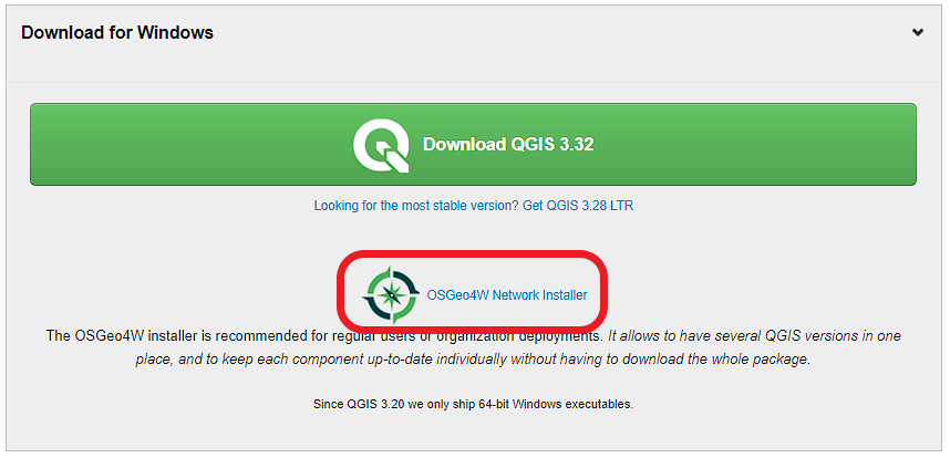 Figure 4.1 Downloading the OSGeo4W installer
 - Click on the link that says "Download OSGeo4W Installer and start it" to downloaded a file called osgeo4w-setup.exe . Then run that file to start the installation.
- Select the "Express Desktop Install" option (Unless you already have OSGeo4W/QGIS installed, then use the Advanced option to ensure you get the latest versions of all packages/tools or pick a different installation folder. If you get errors attempting to run QGIS, you may have to delete your c:\OSGEO4W folder and re-run the installation.)
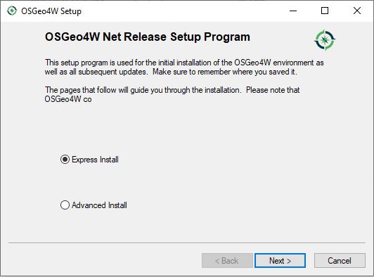 Figure 4.2 Selecting the Express Desktop Install option
 - If asked, select a site from which to install (does not matter which)
- When asked which packages to install, select the options shown in the screenshot below. Apart from that you can accept the default settings on the next pages.
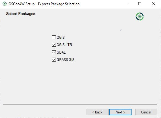 Figure 4.2b Selecting the packages to install
 - Accept the different licenses and run the installation (ignore warnings about corrupted packages if you get them and just click 'Next' if you get warnings about missing dependencies)
Where to find what?
After the installation has finished, you should have a folder called OSGeo4W in the root folder of your C: drive (unless you picked a different folder for the installation). Here we list the main programs from this installation folder that you will need in this lesson:
- C:\OSGeo4W\OSGeo4W.bat - This opens the OSGeo4W shell that can be used for executing python scripts from the command line.
- C:\OSGeo4W\bin\qgis-ltr-bin.exe - This is the main QGIS executable that you need to run for starting QGIS 3.
- C:\OSGeo4W\apps\Qt5\bin\designer.exe - This is the QT Designer executable that you can use for creating Qt5 GUIs in this lesson. If you simply double-click the .exe file in the Windows File Explorer, you will most likely get an DLL related error message because some environment variables won't be set correctly. But you should be able to run the program by opening the OSGeo4W shell and typing the command designer there.
- python-qgis-ltr - As explained further below, you can use this command in the OSGeo4W shell for setting the path and environment variables for running qgis and PyQT5 based Python 3 code as well as executing scripts directly.
Running OSGeo4W shell and commands for qgis and PyQt5 development
When you run OSGeo4W.bat, the OSGeo4W shell will show up looking similar to the normal Windows command line but providing some additional commands that can be listed by typing in "o-help".
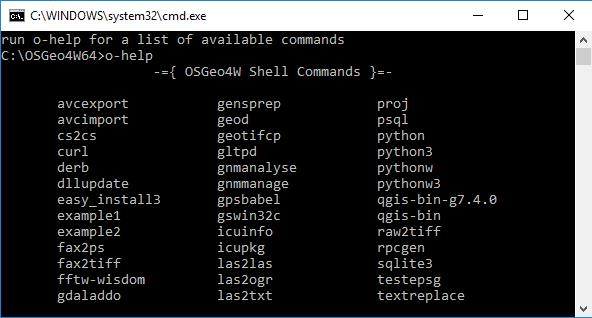
When using the OSGeo4W shell in this lesson, it is best to always execute the command
python-qgis-ltr
first to make sure all environment variables are set up correctly for running qgis and PyQt5 based Python code. The command will start a Python interpreter (recongnizable by the >>> prompt) that you can immediately leave again by typing the command quit() . You can also directly run Python scripts with python-qgis-ltr by writing
python-qgis-ltr xyz.py
rather than just
python xyz.py
You can also use the command pyrcc5 in the OSGeo4W shell for compiling QT5 resource files that we will need later on in this lesson.
Installing geopy package and pandas
Most of the Python packages we will need in this lesson (like PyQt5) are already installed in the Python environment that comes with OSGeo4W/QGIS, but a few additional pieces are necessary. There is one package that we will use for performing distance calculations between WGS84 points in the two walkthroughs of the lesson. The package is called geopy and it needs to be installed first. To do this, please open the OSGeo4W shell and change to Python 3 by running the python-qgis-ltr command followed by quit() as described above, and then run the following pip installation command:
python -m pip install geopy
The package is small, so the installation should only take a couple of seconds. The output you are getting may look slightly different than what is shown in the image below but should indicate that geopy has been installed successfully.
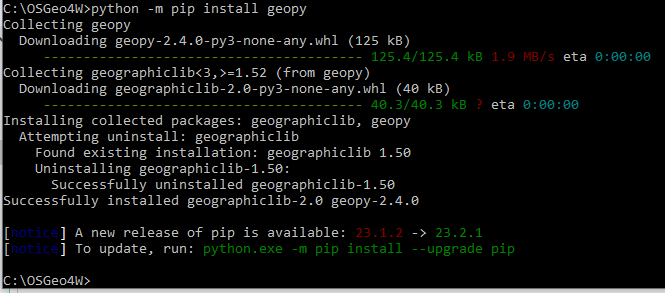
In the practice exercise for this lesson, we will also use pandas. In earlier versions of QGIS/OSGeo4W, pandas wasn't installed by default. To make sure, simply run the following command for installing pandas; most likely it's going to tell you that pandas is already installed:
python -m pip install pandas
Installing the required QGIS plugins
We will need a few QGIS plugins in this lesson, so let's install those as well. Some of these are for the optional part at the end but they are small and installation should be quick, so let's install all of them now. Please follow the instructions below for this:
- Start QGIS
- Go to Plugins -> Manage and Install Plugins in the main menu bar
- Under "Settings", make sure the box next to "Show also experimental plugins" is checked.
- Under "Not installed" look for the following three plugins and install them:
- QuickMapServices (allows for quickly adding basemaps like OSM to a project)
- Plugin Builder 3 (for creating templates for new plugins)
- Plugin Reloader (for reloading a plugin after modifying the code)
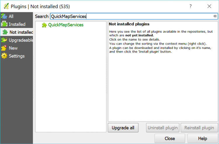
If you now click on "Installed", all three plugins should appear in the list of installed plugins with a checkmark on the left, which indicates that the plugin is activated.
4.4.2 Familiarizing yourself with QGIS
Important note: This lesson has a lot of content and this is one of its less important sections. We included it so that, if you have not worked with QGIS before, you get an idea of where to find what and how things work in QGIS in general. However, since we will mainly be using the QGIS programming API rather than doing things in QGIS itself, we recommend that you go through this section quickly and then maybe come back at the end of the lesson if you have an interest in learning more about QGIS and its interface.
When you open QGIS 3 for the first time, it will look similar to the image below. The main elements are the main menu bar at the top, a number of horizontal toolbars with buttons for different operations below the menu bar, a smaller vertical toolbar on the left side with buttons for adding or creating layers, and then three main windows: a panel with a file browser, a panel that lists the layers in your project (currently empty), and then the main window for displaying the current project. At the very bottom, you can find a status bar displaying information related to the project window such as the scale and coordinate reference system used. Overall, this all looks somewhat similar to ArcGIS Desktop or Pro. All toolbars and panels can be freely moved around, undocked and docked back again, and there are many additional panels and toolbars that can be enabled/disabled either from the main menu under View -> Panels/Toolbars or by doing a right-click on one of the panel title bars or toolbar areas at the top and left.
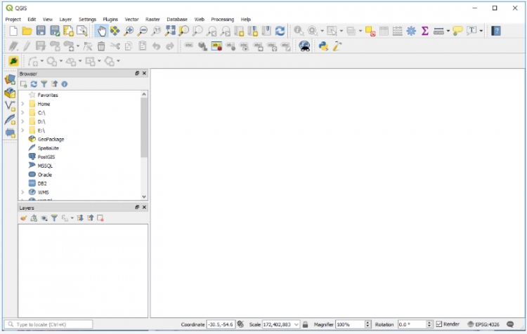
There are several ways to add a data set to a project:
- By navigating to a file in the file browser panel and then double-clicking it.
- By dragging a file from the Windows File Explorer onto the project window or layers panel.
- By clicking the “Open Data Source Manager”
 button, which will open up a dialog with a list of different types of sources on the left including local files, datasets from different databases, and also data sets provided as web services (WMS, WFS, ArcGIS Map Server or Feature Server, etc.).
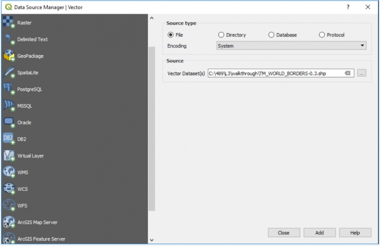
Feel free to try out adding different data sets to the project. Similar to ArcGIS, the coordinate reference system used for the project and project window will be that of the first source added, but of course this can be changed, e.g. by going Project -> Project Properties…. in the menu bar or by left-clicking the CRS field in the status bar. Dragging the layers and the buttons at the top of the Layers panel can be used to arrange the layers in a certain order and group or filter them. We here add the world borders layer from Lesson 3 to the project. The layer now shows up in the project window and the Layers panel. Right-clicking the layer in the Layers panel will provide a number of options for that layer. Double-clicking the layer will directly open the “Layer Properties” dialog with a lot of options to change rendering or other properties of the layer.
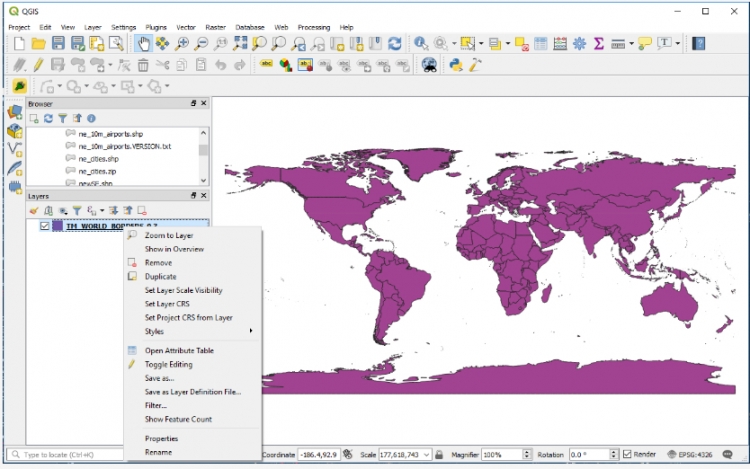
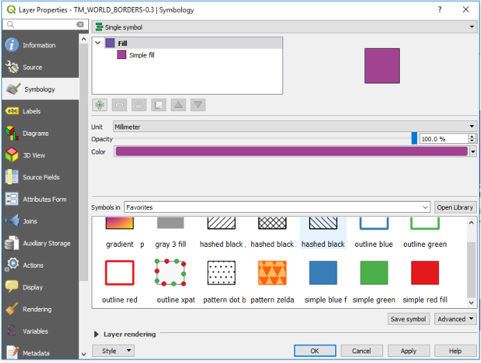
The properties you will most commonly work with are the Symbology and Labels properties. When coming from ArcGIS, working with these dialogs requires a bit of getting used to. Give it a try by attempting to show the world borders layer with a Graduated scheme based on the “AREA” attribute of the layer using a Natural Breaks classification with 8 classes and with labels based on the “NAME” attribute. The result should look somewhat similar to the image below. If you have any problems achieving this, please post on the Lesson 4 discussion forum.
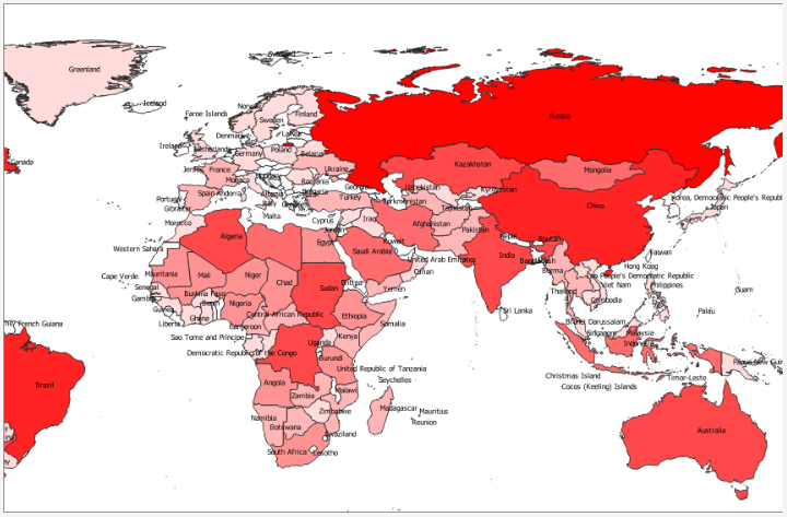
If you want to select features from a layer based on attribute, the Query Builder dialog can be opened by doing a right-click -> Filter … on the layer in the Layers panel. The dialog itself works roughly similar to the corresponding component of ArcGIS. You can check out the attribute table of the layer by doing a right-click -> Open Attribute Table. Working with the attribute table again is roughly similar to ArcGIS. If you want to export a layer as a new data set, you do a right-click -> Export -> Save Features as… . This, for instance, allows for saving only the currently selected features and/or saving the layer in a different format or using a different CRS.
Looking at the main menu bar, we find the main tools for working with Vector and Raster data under the respective submenus. They include typical geoprocessing, data manipulation, and analysis tools. Additional tools can be accessed by opening the Processing Toolbox panel under Processing -> Toolbox. Moreover, QGIS has a plugin interface that allows for writing extensions to QGIS. Plugins can be managed and new plugins can be installed under Plugins -> Manage and Install Plugins, and they can add new entries to menu bar and tool bars. QGIS plugins are written in Python, and you will learn how to do so later on in this lesson. QGIS also has a Python Console (Plugins -> Python Console) that allows for entering and executing Python code that uses the QGIS Python API.
A QGIS project is saved as a .qgz file using Project -> Save or Project -> Save As…. From this menu, you can also open a new project, export the project map in different formats, etc.
One thing that works a bit differently than in ArcGIS is the layout composer component for creating map views of your project including additional elements such as a legend, scale bar, etc. By going Project -> New Print Layout, you can create a new map layout document. This opens up a new window with its own interface that allows you to arrange maps and other elements like images and text in the same way as in a vector graphics or publishing tool. The created layout can just be a single page or span multiple pages and contain different maps. Elements are added to the page with the buttons from the toolbar on the left. A list of all elements is shown in the panel on the top right. The properties of the currently selected element can be accessed and changed with the panel on the bottom right. The simple layout in the image below was created by adding our current map with the add map  button, adding a text element with the add text button
  , and then adding a legend for the current map with the add legend
  button.
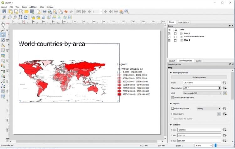
Layouts can be exported as images or PDF files and previously created layouts can be accessed via the Layout Manager under Project -> Layout Manager… or directly be accessed from Project -> Layouts -> … .
This short overview should be enough to get you started but, of course, only covers the basics. This lesson will focus on the QGIS Python API and using it to write programs or plugins for QGIS, rather than on working with the QGIS interface directly. Nevertheless, if you want to learn more about QGIS at some point, the following tutorials covering certain tasks in more detail can be used as a starting point.
More tutorials are available at this QGIS Tutorials and Tips page.
4.5 The QGIS Scripting Interface and Python API
QGIS has a Python programming interface that allows for extending its functionality and for writing scripts that automate QGIS based workflows either inside QGIS or as standalone applications. The Python package that provides this interface is simply called qgis but often referred to as pyQGIS. Its functionality overlaps with what is available in packages that you already know such as arcpy, GDAL/ORG, and the Esri Python API. In the following, we provide a brief introduction to the API so that you are able to perform standard operations like loading and writing vector data, manipulating features and their attributes, and performing selection and geoprocessing operations.
4.5.1 Interacting with Layers Open in QGIS
Let’s start this introduction by writing some code directly in the QGIS Python console and talking about how you can access the layers currently open in QGIS and add new layers to the currently open project. If you don’t have QGIS running at the moment, please start it up and open the Python console from the Plugins menu in the main menu bar.
When you open the Python console in QGIS, the Python qgis package and its submodules are automatically imported as well as other relevant modules including the main PyQt5 modules. In addition, a variable called iface is set up to provide an object of the class QgisInterface1 to interact with the running QGIS environment. The code below shows how you can use that object to retrieve a list of the layers in the currently open map project and the currently active layer. Before you type in and run the code in the console, please add a few layers to an empty project including the TM_WORLD_BORDERS-0.3.shp shapefile that we already used in Section 3.9.1 on GDAL/ORG. We will recreate some of the steps from that section with QGIS here so that you also get a bit of a comparison between the two APIs. The currently active layer is the one selected in the Layers window; please select the world borders layer by clicking on it before you execute the code.
layers = iface.mapCanvas().layers()
for layer in layers:
print(layer)
print(layer.name())
print(layer.id())
print('------')
# If you copy/paste the code - run the part above
# before you run the part below
# otherwise you'll get a syntax error.
activeLayer = iface.activeLayer()
print('active layer: ' + activeLayer.name())
Output (numbers will vary): ...<qgis._core.QgsVectorLayer object at 0x000000666CF22D38> TM_WORLD_BORDERS-0.3 TM_WORLD_BORDERS_0_3_2e5a7cd5_591a_4d45_a4aa_cbba2e639e75 ------ ... active layer: TM_WORLD_BORDERS-0.3
The layers() method of the QgsMapCanvas object we get from calling iface.mapCanvas() returns the currently open layers as a list of objects of the different subclasses of QgsMapLayer. Invoking the name() method of these layer objects gives us the name under which the layer is listed in the Layers window. layer.id() gives us the ID that QGIS has assigned to the layer which in contrast to the name is unique. The iface.activeLayer() method gives us the currently selected layer.
The type() function of a layer can be used to test the type of the layer:
if activeLayer.type() == QgsMapLayer.VectorLayer:
print('This is a vector layer!')
Depending on the type of the layer, there are other methods that we can call to get more information about the layer. For instance, for a vector layer we can use wkbType() to get the geometry type of the layer:
if activeLayer.type() == QgsMapLayer.VectorLayer:
if activeLayer.wkbType() == QgsWkbTypes.MultiPolygon:
print('This layer contains multi-polygons!')
The output you get from the previous command should confirm that the active world borders layer contains multi-polygons, meaning features that can have multiple polygonal parts.
QGIS defines a function dir(…) that can be used to list the methods that can be invoked for a given object. Try out the following two applications of this function:
dir(iface) dir(activeLayer)
To add or remove a layer, we need to work with the QgsProject object for the project currently open in QGIS. We retrieve it like this:
currentProject = QgsProject.instance() print(currentProject.fileName())
The output from the print statement in the second row will probably be the empty string unless you have saved the project. Feel free to do so and rerun the line and you should get the actual file name.
Here is how we can remove the active layer (or any other layer object) from the layer registry of the project (you may have to resize/refresh the map canvas afterwards for the layer to disappear there):
currentProject.removeMapLayer(activeLayer.id())
The following command shows how we can add the world borders shapefile again (or any other feature class we have on disk). Make sure you adapt the path based on where you have the shapefile stored. We first have to create the vector layer object providing the file name and optionally the name to be used for the layer. Then we add that layer object to the project via the addMapLayer(…) method:
layer = QgsVectorLayer(r'C:\489\TM_WORLD_BORDERS-0.3.shp', 'World borders') currentProject.addMapLayer(layer)
Lastly, here is an example that shows you how you can change the symbology of a layer from your code:
renderer = QgsGraduatedSymbolRenderer()
renderer.setClassAttribute('POP2005')
layer.setRenderer(renderer)
layer.renderer().updateClasses(layer, QgsGraduatedSymbolRenderer.Jenks, 5)
layer.renderer().updateColorRamp(QgsGradientColorRamp(Qt.white, Qt.red))
iface.layerTreeView().refreshLayerSymbology(layer.id())
iface.mapCanvas().refreshAllLayers()
Here we create an object of the QgsGraduatedSymbolRenderer class that we want to use to draw the country polygons from our layer using a graduated color approach based on the population attribute ‘POP2005’. The name of the field to use is set via the renderer’s setClassAttribute() method in line 2. Then we make the renderer object the renderer for our world borders layer in line 3. In the next two lines, we tell the renderer (now accessed via the layer method renderer()) to use a Jenks Natural Breaks classification with 5 classes and a gradient color ramp that interpolates between the colors white and red. Please note that the colors used as parameters here are predefined instances of the Qt5 class QColor. Changing the symbology does not automatically refresh the map canvas or layer list. Therefore, in the last two lines, we explicitly tell the running QGIS environment to refresh the symbology of the world borders layer in the Layers tree view (line 6) and to refresh the map canvas (line 7). The result should look similar to the figure below (with all other layers removed).
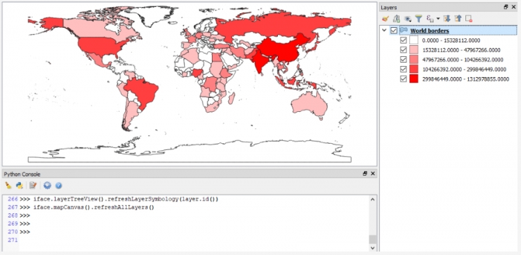
You will get to see another example of interacting with the layers open in QGIS and setting the symbology (for point and line layers in this case) in Section 4.12 where we take the code from this lesson's walkthrough and turn it into a QGIS plugin.
[1] The qgis Python module is a wrapper around the underlying C++ library. The documentation pages linked in this section are those of the C++ version but the names of classes and available functions and methods are the same.
4.5.2 Accessing the Features of a Layer
Let’s keep working with the world borders layer open in QGIS for a bit, looking at how we can access the individual features in a layer and select features by attribute. The following piece of code shows you how we can loop through all the features with the help of the layer’s getFeatures() method:
for feature in layer.getFeatures():
print(feature)
print(feature.id())
print(feature['NAME'])
print('-----')
Output: <qgis._core.QgsFeature object at 0x...> 0 Antigua and Barbuda ----- <qgis._core.QgsFeature object at 0x...> 1 Algeria ----- <qgis._core.QgsFeature object at 0x...> 2 Azerbaijan ----- <qgis._core.QgsFeature object at 0x...> 3 Albania ----- ...
Features are represented as objects of the class QgsFeature in QGIS. So, for each iteration of the for-loop in the previous code example, variable feature will contain a QgsFeature object. Features are numbered with a unique ID that you can obtain by calling the method id() as we are doing in this example. Attributes like the NAME attribute of the world borders polygons can be accessed using the attribute name as the key as also demonstrated above.
Like in most GIS software, a layer can have an active selection. When the layer is open in QGIS, the selected features are highlighted. The layer method selectAll() allows for selecting all features in a layer and removeSelection() can be used to clear the selection. Give this a try by running the following two commands in the QGIS Python console and watch how all countries become selected and then deselected again.
layer.selectAll() layer.removeSelection()
The method selectByExpression() allows for selecting features based on their properties with a SQL query string that has the same format as in ArcGIS. Use the following command to select all features from the layer that have a value larger than 300,000 in the AREA column of the attribute table. The result should look as in the figure below.
layer.selectByExpression('"AREA" > 300000')
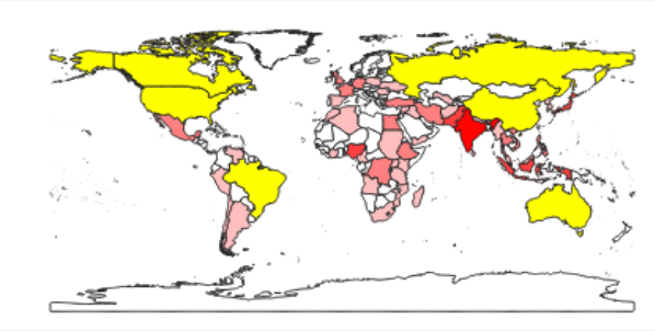
While there can only be one active selection for a layer, you can create as many subgroups of features from a layer as you want by calling getFeatures(…) with a parameter that is an object of the class QgsFeatureRequest and that has been given a filter expression via its setFilterExpression(…) method. The filter expression can be again an SQL query string. The following code creates a subgroup that will only contain the polygon for Canada. When you run it, this will not change the active selection that you see for that layer in QGIS but variable selectionName now provides access to the subgroup with just that one polygon. We get that first (and only) polygon by calling the __next__() method of selectionName and then print out some information about this particular polygon feature.
selectionName = layer.getFeatures(QgsFeatureRequest().setFilterExpression('"NAME" = \'Canada\''))
feature = selectionName.__next__()
print(feature['NAME'] + "-" + str(feature.id()))
print(feature.geometry())
print(feature.geometry().asWkt())
Output: Canada – 23 <qgis._core.QgsGeometry object at 0x...> MultiPolygon (((-65.61361699999997654 43.42027300000000878,...)))
The first print statement in this example works in the same way as you have seen before to get the name attribute and id of the feature. The method geometry() gives us the geometric object for this feature as an instance of the QgsGeometry class and calling the method asWkt() gives us a WKT string representation of the multi-polygon geometry. You can also use a for-loop to iterate through the features in a subgroup created in this way. The method rewind() can be used to reset the iterator to the beginning so that when you call __next__() again, it will again give you the first feature from the subgroup.
When you have the geometry object and know what type of geometry it is, you can use the methods asPoint(), asPolygon(), asPolyline(), asMultiPolygon(), etc. to get the geometry as a Python data structure, e.g. in the case of multi-polygons as a list of lists of lists with each inner list containing tuples of the point coordinates for one polygonal component.
print(feature.geometry().asMultiPolygon())
[[[(-65.6136, 43.4203), (-65.6197,43.4181), … ]]]
Here is another example to demonstrate that we can work with several different subgroups of features at the same time. This time we request all features from the layer that have a POP2005 value larger than 50,000,000.
selectionPopulation = layer.getFeatures(QgsFeatureRequest().setFilterExpression('"POP2005" > 50000000'))
If we ever want to use a subgroup like this to create the active selection for the layer from it, we can use the layer method selectByIds(…) for this. The method requires a list of feature IDs and will then change the active selection to these features. In the following example, we use a simple list comprehension to create the ID list from the subgroup in our variable selectionPopulation:
layer.selectByIds([f.id() for f in selectionPopulation])
When running this command you should notice that the selection of the features in QGIS changes to look like in the figure below.
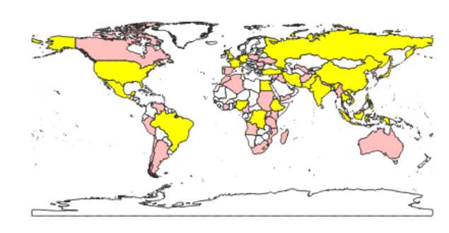
Let’s save the currently selected features as a new file. We use the GeoPackage format (GPKG) for this, which is more modern than the shapefile format, but you can easily change the command below to produce a shapefile instead; simply change the file extension to “.shp” and replace “GPKG” with “ESRI Shapefile”. The function we will use for writing the layer to disk is called writeAsVectorFormat(…) and it is defined in the class QgsVectorFileWriter. Please note that this function has been declared "deprecated", meaning it may be removed in future versions and it is recommended that you do not use it anymore. In versions up to QGIS 3.16 (the current LTR version that most likely you are using right now), you are supposed to use writeAsVectorFormatV2(...) instead; however, there have been issues reported with that function and it is already replaced by writeAsVectorFormatV3(...) in versions >3.16 of QGIS. Therefore, we have decided to stick with writeAsVectorFormat(…) while things are still in flux. The parameters we give to writeAsVectorFormat(…) are the layer we want to save, the name of the output file, the character encoding to use, the spatial reference to use (we simply use the one that our layer is in), the format (“GPKG”), and True for signaling that only the selected features should be saved in the new data set. Adapt the path for the output file as you see fit and then run the command:
QgsVectorFileWriter.writeAsVectorFormat(layer, r'C:\489\highPopulationCountries.gpkg', 'utf-8', layer.crs(),'GPKG', True)
If you add the new file produced by this command to your QGIS project, it should only contain the polygons for the countries we selected based on their population values.
For changing the attribute values of a feature, we need to work with the “data provider” object of the layer. We can access it via the layer’s dataProvider() method:
dataProvider = layer.dataProvider()
Let’s say we want to change the POP2005 value for Canada to 1 (don’t ask what happened!). For this, we also need the index of the POP2005 column which we can get by calling the data provider’s fieldNameIndex() method:
populationColumnIndex = dataProvider.fieldNameIndex('POP2005')
To change the attribute value we call the method changeAttributeValues(…) of the data provider object providing a dictionary as parameter that maps feature IDs to dictionaries which in turn map column indices to new values. The inner dictionary that maps column indices to values is defined in a separate variable newValueDictionary.
newValueDictionary = { populationColumnIndex : 1 }
dataProvider.changeAttributeValues( { feature.id(): newValueDictionary } )
In this simple example, the outer dictionary contains only a single key-value pair with the ID of the feature for Canada as key and another dictionary as value. The inner dictionary also only contains a single key-value pair consisting of the index of the population column and its new value 1. Both dictionaries can have multiple entries to simultaneously change multiple values of multiple features. After running this command, check out the attributes of Canada, either via the QGIS Identify tool or in the attribute table of the layer. You will see that the population value in the layer now has been changed to 1 (the same holds for the underlying shapefile). Let’s set the value back to what it was with the following command:
dataProvider.changeAttributeValues( { feature.id(): { populationColumnIndex : 32270507 } } )
4.5.3 Creating Features and Geometric Operations
For the final part of this section, let’s switch from the Python console in QGIS to writing a standalone script that uses qgis. You can use your editor of choice to write the script and then execute the .py file from the OSGeo4W shell (see again Section 4.4.1) with all environment variables set correctly for a qgis and QT5 based program.
We are going to repeat the task from Section 3.9.1 of creating buffers around the centroids of the countries within a rectangular (in terms of WGS 84 coordinates) area around southern Africa. We will produce two new vector GeoPackage files: a point based one with the centroids and a polygon based one for the buffers. Both data sets will only contain the country name as their only attribute.
We start by importing the modules we will need and creating a QApplication() (handled by qgis.core.QgsApplication) for our program that qgis can run in (even though the program does not involve any GUI).
Important note: When you later write you own qgis programs (e.g. in the L4 homework assignment), make sure that you always "import qgis" first before using any other qgis related import statements such as "import qgis.core". We are not sure why this is needed, but the other imports will most likely fail tend to fail without "import qgis" coming first.
import os, sys import qgis import qgis.core
To use qgis in our software, we have to initialize it and we need to tell it where the actual QGIS installation is located. To do this, we use the function getenv(…) of the os module to get the value of the environmental variable “QGIS_PREFIX_PATH” which will be correctly defined when we run the program from the OSGeo4W shell. Then we create an instance of the QgsApplication class and call its initQgis() method.
qgis_prefix = os.getenv("QGIS_PREFIX_PATH")
qgis.core.QgsApplication.setPrefixPath(qgis_prefix, True)
qgs = qgis.core.QgsApplication([], False)
qgs.initQgis()
Now we can implement the main functionality of our program. First, we load the world borders shapefile into a layer (you may have to adapt the path!).
layer = qgis.core.QgsVectorLayer(r'C:\489\TM_WORLD_BORDERS-0.3.shp')
Then we create the two new layers for the centroids and buffers. These layers will be created as new in-memory layers and later written to GeoPackage files. We provide three parameters to QgsVectorLayer(…): (1) a string that specifies the geometry type, coordinate system, and fields for the new layer; (2) a name for the layer; and (3) the string “memory” which tells the function that it should create a new layer in memory from scratch (rather than reading a data set from somewhere else as we did earlier).
centroidLayer = qgis.core.QgsVectorLayer("Point?crs=" + layer.crs().authid() + "&field=NAME:string(255)", "temporary_points", "memory")
bufferLayer = qgis.core.QgsVectorLayer("Polygon?crs=" + layer.crs().authid() + "&field=NAME:string(255)", "temporary_buffers", "memory")
The strings produced for the first parameters will look like this: “Point?crs=EPSG:4326&field=NAME:string(255)” and “Polygon?crs=EPSG:4326&field=NAME:string(255)”. Note how we are getting the EPSG string from the world border layer so that the new layers use the same coordinate system, and how an attribute field is described using the syntax “field=<name of the field>:<type of the field>". When you want your layer to have more fields, these have to be separated by additional & symbols like in a URL.
Next, we set up variables for the data providers of both layers that we will need to create new features for them. The new features will be collected in two lists, centroidFeatures and bufferFeatures.
centroidProvider = centroidLayer.dataProvider() bufferProvider = bufferLayer.dataProvider() centroidFeatures = [] bufferFeatures = []
Then, we create the polygon geometry for our selection area from a WKT string as in Section 3.9.1:
areaPolygon = qgis.core.QgsGeometry.fromWkt('POLYGON ( (6.3 -14, 52 -14, 52 -40, 6.3 -40, 6.3 -14) )')
In the main loop of our program, we go through all the features in the world borders layer, use the geometry method intersects(…) to test whether the country polygon intersects with the area polygon, and, if yes, create the centroid and buffer features for the two layers from the input feature.
for feature in layer.getFeatures():
if feature.geometry().intersects(areaPolygon):
centroid = qgis.core.QgsFeature()
centroid.setAttributes([feature['NAME']])
centroid.setGeometry(feature.geometry().centroid())
centroidFeatures.append(centroid)
buffer = qgis.core.QgsFeature()
buffer.setAttributes([feature['NAME']])
buffer.setGeometry(feature.geometry().centroid().buffer(2.0,100))
bufferFeatures.append(buffer)
Note how in both cases (centroids and buffers), we first create a new QgsFeature object, then use setAttributes(…) to set the NAME attribute to the name of the country, and then use setGeometry(…) to set the geometry of the new feature either to the centroid derived by calling the centroid() method or to the buffered centroid created by calling the buffer(…) method of the centroid point. As a last step, the new features are added to the respective lists. Finally, all features in the two lists are added to the layers after the for-loop has been completed. This happens with the following two commands:
centroidProvider.addFeatures(centroidFeatures) bufferProvider.addFeatures(bufferFeatures)
Lastly, we write the content of the two in-memory layers to GeoPackage files on disk. This works in the same way as in previous examples. Again, you might want to adapt the output paths.
qgis.core.QgsVectorFileWriter.writeAsVectorFormat(centroidLayer, r'C:\489\centroids.gpkg', "utf-8", layer.crs(), "GPKG") qgis.core.QgsVectorFileWriter.writeAsVectorFormat(bufferLayer, r'C:\489\buffers.gpkg', "utf-8", layer.crs(), "GPKG")
Since we are now done with using QGIS functionalities (and actually the entire program), we clean up by calling the exitQgis() method of the QgsApplication, freeing up resources that we don’t need anymore.
qgs.exitQgis()
If you run the program from the OSGeo4W shell and then open the two produced output files in QGIS, the result should look as shown in the image below.
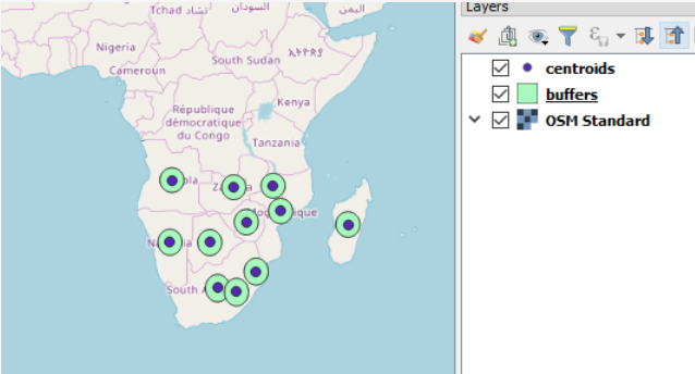
4.5.4 (Geo)processing
QGIS has a toolbox system and visual workflow building component somewhat similar to ArcGIS and its Model Builder. It is called the QGIS processing framework and comes in the form of a plugin called Processing that is installed by default. You can access it via the Processing menu in the main menu bar. All algorithms from the processing framework are available in Python via a QGIS module called processing. They can be combined to solve larger analysis tasks in Python and can also be used in combination with the other qgis methods discussed in the previous sections.
We can get a list of all processing algorithms currently registered with QGIS with the command QgsApplication.processingRegistry().algorithms(). Each processing object in the returned list has an identifying name that you can get via its id() method. The following command, which you can try out in the QGIS Python console, uses this approach to print the names of all algorithms that contain the word “clip”:
[x.id() for x in QgsApplication.processingRegistry().algorithms() if "clip" in x.id()]
Output: ['gdal:cliprasterbyextent', 'gdal:cliprasterbymasklayer','gdal:clipvectorbyextent', 'gdal:clipvectorbypolygon', 'native:clip', 'saga:clippointswithpolygons', 'saga:cliprasterwithpolygon', 'saga:polygonclipping']
As you can see, there are processing versions of algorithms coming from different sources, e.g. natively built into QGIS vs. algorithms based on GDAL. The function algorithmHelp(…) allows you to get some documentation on an algorithm and its parameters. Try it out with the following command:
processing.algorithmHelp("native:clip")
To run a processing algorithm, you have to use the run(…) function and provide two parameters: the id of the algorithm and a dictionary that contains the parameters for the algorithm as key-value pairs. run(…) returns a dictionary with all output parameters of the algorithm. The following example illustrates how processing algorithms can be used to solve the task of clipping a points of interest shapefile to the area of El Salvador, reusing the two data sets from homework assignment 2 (Section 2.10). This example is intended to be run as a standalone program again and most of the code is required to set up the QGIS environment needed, including initializing the Processing environment.
The start of the script looks like in the example from the previous section:
import os,sys
import qgis
import qgis.core
qgis_prefix = os.getenv("QGIS_PREFIX_PATH")
qgis.core.QgsApplication.setPrefixPath(qgis_prefix, True)
qgs = qgis.core.QgsApplication([], False)
qgs.initQgis()
After, creating the QGIS environment, we can now initialize the processing framework. To be able to import the processing module we have to make sure that the plugins folder is part of the system path; we do this directly from our code. After importing processing, we have to initialize the Processing environment and we also add the native QGIS algorithms to the processing algorithm registry.
# Be sure to change the path to point to where your plugins folder is located # it may not be the same as this one. sys.path.append(r"C:\OSGeo4W\apps\qgis-ltr\python\plugins") import processing from processing.core.Processing import Processing Processing.initialize() qgis.core.QgsApplication.processingRegistry().addProvider(qgis.analysis.QgsNativeAlgorithms())
Next, we create input variables for all files involved, including the output files we will produce, one with the selected country and one with only the POIs in that country. We also set up input variables for the name of the country and the field that contains the country names.
poiFile = r'C:\489\L2\assignment\OSMpoints.shp' countryFile = r'C:\489\L2\assignment\countries.shp' pointOutputFile = r'C:\489\L2\assignment\pointsInCountry.shp' countryOutputFile = r'C:\489\L2\assignment\singleCountry.shp' nameField = "NAME" countryName = "El Salvador"
Now comes the part in which we actually run algorithms from the processing framework. First, we use the qgis:extractbyattribute algorithm to create a new shapefile with only those features from the country data set that satisfy a particular attribute query. In the dictionary with the input parameters for the algorithm, we specify the name of the input file (“INPUT”), the name of the query field (“FIELD”), the comparison operator for the query (0 here stands for “equal”), and the value to which we are comparing (“VALUE”). Since the output will be written to a new shapefile, we don’t really need the output dictionary that we get back from calling run(…) but the print statement shows how this dictionary in this case contains the name of the output file under the key “OUTPUT”.
output = processing.run("qgis:extractbyattribute", { "INPUT": countryFile, "FIELD": nameField, "OPERATOR": 0, "VALUE": countryName, "OUTPUT": countryOutputFile })
print(output['OUTPUT'])
To perform the clip operation with the new shapefile from the previous step, we use the “native:clip” algorithm. The input paramters are the input file (“INPUT”), the clip file (“OVERLAY”), and the output file (“OUTPUT”). Again, we are just printing out the content stored under the “OUTPUT” key in the returned dictionary. Finally, we exit the QGIS environment.
output = processing.run("native:clip", { "INPUT": poiFile, "OVERLAY": countryOutputFile, "OUTPUT": pointOutputFile })
print(output['OUTPUT'])
qgs.exitQgis()
Below is how the resulting two layers should look when shown in QGIS in combination with the original country layer.
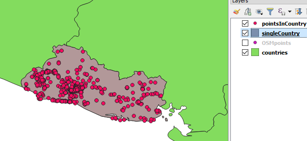
In this section, we showed you how to perform common GIS operations with the QGIS Python API. Once again we have to say that we are only scratching the surface here; the API is much more complex and powerful, and there is hardly anything you cannot do with it. What we have shown you will be sufficient to understand the code from the two walkthroughs of this lesson, but, if you want more, below are some links to further examples. Keep in mind though that since QGIS 3 is not that old yet, some of the examples on the web have been written for QGIS 2.x. While many things still work in the same way in QGIS 3, you may run into situations in which an example won’t work and needs to be adapted to be compatible with QGIS 3.
4.6 Object-Oriented Programming in Python
GEOG 485 already described some of the fundamental ideas of object-oriented programming and you have been using objects of classes defined in different Python packages like arcpy quite a bit. For instance, you have been creating new objects of the arcpy Point or Array classes by writing something like
p = arcpy.Point() points = arcpy.Array()
You have also been accessing properties of the objects created, e.g. by writing
p.X
... to get the x coordinate of the Point object stored in variable p. And you have been invoking methods of objects, for instance the add(…) method to add a point to the Array stored in variable points:
points.add(p)
What we did not cover in GEOG485 is how to define your own classes in Python, derive new classes from already existing ones to create class hierarchies, and use these ideas to build larger software applications with a high degree of readability, maintainability, and reusability. All these things will be covered in this and the next section and put into practice throughout the rest of this lesson.
4.6.1 Classes, Objects, and Methods
Let’s recapitulate a bit: the underlying perspective of object-oriented programming is that the domain modeled in a program consists of objects belonging to different classes. If your software models some part of the real world, you may have classes for things like buildings, vehicles, trees, etc. and then the objects (also called instances) created from these classes during run-time represent concrete individual buildings, vehicles, or trees with their specific properties. The classes in your software can also describe non real-world and often very abstract things like a feature layer or a random number generator.
Class definitions specify general properties that all objects of that class have in common, together with the things that one can do with these objects. Therefore, they can be considered blueprints for the objects. Each object at any moment during run-time is in a particular state that consists of the concrete values it has for the properties defined in its class. So, for instance, the definition of a very basic class Car may specify that all cars have the properties owner, color, currentSpeed, and lightsOn. During run-time we might then create an object for “Tom’s car” in variable carOfTom with the following values making up its state:
carOfTom.owner = "Tom" carOfTom.color = "blue" carOfTom.currentSpeed = 48 (mph) carOfTom.lightsOn = False
While all objects of the same class have the same properties (also called attributes or fields), their values for these properties may vary and, hence, they can be in different states. The actions that one can perform with a car or things that can happen to a car are described in the form of methods in the class definition. For instance, the class Car may specify that the current speed of cars can be changed to a new value and that lights can be turned on and off. The respective methods may be called changeCurrentSpeed(…), turnLightsOn(), and turnLightsOff(). Methods are like functions but they are explicitly invoked on an object of the class they are defined in. In Python this is done by using the name of the variable that contains the object, followed by a dot, followed by the method name:
carOfTom.changeCurrentSpeed(34) # change state of Tom’s car to current speed being 34mph carOfTom.turnLightsOn() # change state of Tom’s car to lights being turned on
The purpose of methods can be to update the state of the object by changing one or several of its properties as in the previous two examples. It can also be to get information about the state of the car, e.g. are the lights turned on? But it can also be something more complicated, e.g. performing a certain driving maneuver or fuel calculation.
In object-oriented programming, a program is perceived as a collection of objects that interact by calling each other’s methods. Object-oriented programming adheres to three main design principles:
- Encapsulation: Definitions related to the properties and methods of any class appear in a specification that is encapsulated independently from the rest of the software code and properties are only accessible via a well-defined interface, e.g. via the defined methods.
- Inheritance: Classes can be organized hierarchically with new classes being derived from previously defined classes inheriting all the characteristics of the parent class but potentially adding specialized properties or specialized behavior. For instance, our class Car could be derived from a more general class Vehicle adding properties and methods that are specific for cars.
- Polymorphism: Inherited classes can change the behavior of methods by overwriting them and the code executed when such a method is invoked for an object then depends on the class of that object.
We will talk more about inheritance and polymorphism in section 4.8. All three principles aim at improving reusability and maintainability of software code. These days, most software is created by mainly combining parts that already exist because that saves time and costs and increases reliability when the re-used components have already been thoroughly tested. The idea of classes as encapsulated units within a program increases reusability because these units are then not dependent on other code and can be moved over to a different project much more easily.
For now, let’s look at how our simple class Car can be defined in Python.
class Car():
def __init__(self):
self.owner = 'UNKNOWN'
self.color = 'UNKNOWN'
self.currentSpeed = 0
self.lightsOn = False
def changeCurrentSpeed(self,newSpeed):
self.currentSpeed = newSpeed
def turnLightsOn(self):
self.lightsOn = True
def turnLightsOff(self):
self.lightsOn = False
def printInfo(self):
print('Car with owner = {0}, color = {1}, currentSpeed = {2}, lightsOn = {3}'.format(self.owner, self.color, self.currentSpeed, self.lightsOn))
Here is an explanation of the different parts of this class definition: each class definition in Python starts with the keyword ‘class’ followed by the name of the class (‘Car’) followed by parentheses that may contain names of classes that this class inherits from, but that’s something we will only see later on. The rest of the class definition is indented to the right relative to this line.
The rest of the class definition consists of definitions of the methods of the class which all look like function definitions but have the keyword ‘self’ as the first parameter, which is an indication that this is a method. The method __init__(…) is a special method called the constructor of the class. It will be called when we create a new object of that class like this:
carOfTom = Car() # uses the __init__() method of Car to create a new Car object
In the body of the constructor, we create the properties of the class Car. Each line starting with “self.<name of property> = ...“ creates a so-called instance variable for this car object and assigns it an initial value, e.g. zero for the speed. The instance variables describing the state of an object are another type of variable in addition to global and local variables that you already know. They are part of the object and exist as long as that object exists. They can be accessed from within the class definition as “self.<name of the instance variable>” which happens later in the definitions of the other methods, namely in lines 10, 13, 16 and 19. If you want to access an instance variable from outside the class definition, you have to use <name of variable containing the object>.<name of the instance variable>, so, for instance:
print(carOfTom.lightsOn) # will produce the output False because right now this instance variable still has its default value
The rest of the class definition consists of the methods for performing certain actions with a Car object. You can see that the already mentioned methods for changing the state of the Car object are very simple. They just assign a new value to the respective instance variable, a new speed value that is provided as a parameter in the case of changeCurrentSpeed(…) and a fixed Boolean value in the cases of turnLightsOn() and turnLightsOff(). In addition, we added a method printInfo() that prints out a string with the values of all instance variables to provide us with all information about a car’s current state. Let us now create a new instance of our Car class and then use some of its methods:
carOfSue = Car() carOfSue.owner = 'Sue' carOfSue.color = 'white' carOfSue.changeCurrentSpeed(41) carOfSue.turnLightsOn() carOfSue.printInfo()
Output: Car with owner = Sue, color = white, currentSpeed = 41, lightsOn = True
Since we did not define any methods to change the owner or color of the car, we are directly accessing these instance variables and assigning new values to them in lines 2 and 3. While this is okay in simple examples like this, it is recommended that you provide so-called getter and setter methods (also called accessor and mutator methods) for all instance variables that you want the user of the class to be able to read (“get”) or change (“set”). The methods allow the class to perform certain checks to make sure that the object always remains in an allowed state. How about you go ahead and for practice create a second car object for your own car (or any car you can think of) in a new variable and then print out its information?
A method can call any other method defined in the same class by using the notation “self.<name of the method>(...)”. For example, we can add the following method randomSpeed() to the definition of class Car:
def setRandomSpeed(self):
self.changeCurrentSpeed(random.randint(0,76))
The new method requires the “random” module to be imported at the beginning of the script. The method generates a random number and then uses the previously defined method changeCurrentSpeed(…) to actually change the corresponding instance variable. In this simple example, one could have simply changed the instance variable directly but in more complex cases changes to the state can require more code so that this approach here actually avoids having to repeat that code. Give it a try and add some lines to call this new method for one of the car objects and then print out the info again.
4.6.2 Constructors with parameters and defining the == and < operators
It can be a bit cumbersome to use methods or assignments to set all the instance variables to the desired initial values after a new object has been created. Instead, one would rather like to pass initial values to the constructor and get back an object with these values for the instance variables. It is possible to do so in Python by adding additional parameters to the constructor. Go ahead and change the definition of the constructor in class Car to the following version:
def __init__(self, owner = 'UNKNOWN', color = 'UNKNOWN', currentSpeed = 0, lightsOn = False):
self.owner = owner
self.color = color
self.currentSpeed = currentSpeed
self.lightsOn = lightsOn
Please note that we here used identical names for the instance variables and corresponding parameters of the constructor used for providing the initial values. However, these are still distinguishable because instance variables always have the prefix “self.”. In this new version of the constructor we are using keyword arguments for each of the properties to provide maximal flexibility to the user of the class. The user can now use any combination of providing their own initial values or using the default values for these properties. Here is how to re-create Sue’s car by providing values for all the properties:
carOfSue = Car(owner='Sue', color='white', currentSpeed = 41, lightsOn = True) carOfSue.printInfo()
Output: Car with owner = Sue, color = white, currentSpeed = 41, lightsOn = True
Here is a version in which we only specify the owner and the speed. Surely you can guess what the output will look like.
carOfSue = Car(owner='Sue', currentSpeed = 41) carOfSue.printInfo()
In addition to __init__(…) for the constructor, there is another special method called __str__(). This method is called by Python when you either explicitly convert an object from that class to a string using the Python str(…) function or implicitly, e.g. when printing out the object with print(…). Try out the following two commands for Sue’s car and see what output you get:
print(str(carOfSue)) print(carOfSue)
Now add the following method to the definition of class Car:
def __str__(self):
return 'Car with owner = {0}, color = {1}, currentSpeed = {2}, lightsOn = {3}'.format(self.owner, self.color, self.currentSpeed, self.lightsOn)
Now repeat the two commands from above and look at the difference. The output should now be the following line repeated twice:
Car with owner = Sue, color = UNKNOWN, currentSpeed = 41, lightsOn = False
For implementing the method, we simply used the same string that we were printing out from the printInfo() method. In principal, this method is not really needed anymore now and could be removed from the class definition.
Objects can be used like any other value in Python code. Actually, everything in Python is an object, even primitive data types like numbers and Boolean values. That means we can …
- use objects as parameters of functions and methods (you will see an example of this with the function stopCar(…) defined below),
- return objects as the return value of a function or method,
- store objects inside sequences or containers, for instance in lists like this: carList = [ carOfTom, carOfSue, Car(owner = 'Mike'],
- store objects in instance variables of other objects.
To illustrate this last point, we can add another class to our car example, one for representing car manufacturers:
class Manufacturer():
def __init__(self, name):
self.name = name
Usually such a class would be much more complex, containing additional properties for describing a concrete car manufacturer. But we keep things very simple here and say that the only property is the name of the manufacturer. We now modify the beginning of the definition of class Car so that another instance variable is created called self.manufacturer. This is used for storing an object of class Manufacturer inside each Car object for representing the manufacturer of that particular car. For parameters that are objects of classes, it is common to use the special value None as the default value when the parameter is not provided.
class Car():
def __init__(self, manufacturer = None, owner = 'UNKNOWN', color = 'UNKNOWN', currentSpeed = 0, lightsOn = False):
self.manufacturer = manufacturer
self.owner = owner
self.color = color
self.currentSpeed = currentSpeed
self.lightsOn = lightsOn
The rest of the class definition can stay the same although we would typically change the __str__(...) method to include this new instance variable. The following code shows how to create a new Car object by first creating a Manufacturer object with name 'Chrysler'. This object could also come from a predefined list or dictionary of car manufacturer objects if we want to be able to use the same Manufacturer object for several cars. Then we use this object for the manufacturer keyword argument of the Car constructor. As a result, this object gets assigned to the manufacturer instance variable of the car as reflected by the output from the final print statement.
m = Manufacturer('Chrysler')
carOfFrank = Car(manufacturer = m, owner = 'Frank', currentSpeed = 70)
print(carOfFrank.manufacturer.name)
Output: Chrysler
Note how in the last line of the example above, we chain things together via dots starting from the variable containing the car object (carOfFrank), followed by the name of an instance variable (manufacturer) of class Car, followed by the name of an instance variable of class Manufacturer (name): carOfFrank.manufacturer.name . This is also something you have probably seen before, for instance as “describeObject.SpatialReference.Name” when accessing the name of the spatial reference object that is stored inside an arcpy Describe object.
We briefly discussed in Section 4.2 when talking about collections that when defining our own classes we may have to provide definitions of comparison operators like == and < for them to work as we wish when placed into a collection. So a question for instance would be, when should two car objects be considered to be equal? We could take the standpoint that they are equal if the values of all instance variables are equal. Or it could make sense for a particular application to define that two Car objects are equal if the name of the owner and the manufacturer are equal. If our instance variables would include the license plate number that would obviously make for a much better criterion. Similarly, let us say we want to keep our Car objects in a priority queue sorted by their current speed values. In that case, we need to define the < comparison operator so that car A < car B holds if the value of the currentSpeed variable of A is smaller than that of B.
The meaning of the == operator is defined via a special method called __eq__(…) for “equal”, while that of the < operator is defined in a special method called __lt__(…) for “less than”. The following code example extends the most recent version of our class Car with a definition of the __eq__(…) method based on the idea that cars should be treated as equal if owner and manufacturer are equal. It then uses a Python list with a single car object and another car object with the same owner and manufacturer but different speed to illustrate that the new definition works as intended for the list operations “in” and index(…).
class Car():
… # just add the method below to the previous definition of the class
def __eq__(self, otherCar):
return self.owner == otherCar.owner and self.manufacturer == otherCar.manufacturer
m = 'Chrysler'
carList = [ Car(owner='Sue', currentSpeed = 41, manufacturer = m) ]
car = Car(owner='Sue', currentSpeed = 0, manufacturer = m)
if car in carList:
print('Already contained in the list')
print(carList.index(car))
Output: Already contained in the list 0
Note that __eq__(…) takes another Car object as parameter and then simply compares the values of the owner and manufacturer instance variables of the Car object the method was called for with the corresponding values of that other Car object. The output shows that Python considers the car to be already located in the list as the first element, even though these are actually two different car objects with different speed values. This is because these operations use the new definition of the == operator for objects of our class Car that we provided with the method __eq__(...).
You now know the basics of writing own classes in Python and how to instantiate them and use the created objects. To wrap up this section, let’s come back to a topic that we already discussed in Section 1.4 of Lesson 1. Do you remember the difference between mutable and immutable objects when given as a parameter to functions? Mutable objects like lists used as parameters can be changed within the function. All objects that we create from classes are also mutable, so you can in principle write code like this:
def stopCar(car): car.currentSpeed = 0 stopCar(carOfFrank) print(carOfFrank)
When stopCar(...) is called, the parameter car will refer to the same car object that variable carOfFrank is referring to. Therefore, all changes made to that object inside the function referring to variable car will be reflected by the final print statement for carOfFrank showing a speed of 0. What we have not discussed so far is that there is a second situation where this is important, namely when making an assignment. You may think that when you write something like
anotherCar = carOfFrank
a new variable will be created and a copy of the car object in variable carOfFrank will be assigned to that variable so that you can make changes to the instance variables of that object without changing the object in carOfFrank. However, that is only how it works for immutable values. Instead, after the assignment, both variables will refer to the same Car object in memory. Therefore, when you add the following commands
anotherCar.color = 'green' anotherCar.changeCurrentSpeed(12) print(carOfFrank)
The output will be:
Car with owner = Frank, color = green, currentSpeed = 12, lightsOn = False
It works in the same way for all mutable objects, so also for lists for example. If you want to create an independent copy of a mutable object, the module copy from the Python standard library contains the functions copy(…) and deepcopy(…) to explicitly create copies. The difference between the two functions is explained in the documentation and only plays a role when the object to be copied contains other objects, e.g. if you want to make a copy of a list of Car objects.
4.7 Inheritance, Class Hierarchies and Polymorphism
We already mentioned building class hierarchies via inheritance and polymorphism as two main principles of object-oriented programming in addition to encapsulation. To introduce you to these concepts, let us start with another exercise in object-oriented modeling and writing classes in Python. Imagine that you are supposed to write a very basic GIS or vector drawing program that only deals with geometric features of three types: circles, and axis-aligned rectangles and squares. You need the ability to store and manage an arbitrary number of objects of these three kinds and be able to perform simple operations with these objects like computing their area and perimeter and moving the objects to a different position. How would you write the classes for these three kinds of geometric objects?
Let us start with the class Circle: a circle in a two-dimensional coordinate system is typically defined by three values, the x and y coordinates of the center of the circle and its radius. So these should become the properties (= instance variables) of our Circle class and for computing the area and perimeter, we will provide two methods that return the respective values. The method for moving the circle will take the values by how much the circle should be moved along the x and y axes as parameters but not return anything.
import math
class Circle():
def __init__(self, x = 0.0, y = 0.0, radius = 1.0):
self.x = x
self.y = y
self.radius = radius
def computeArea(self):
return math.pi * self.radius ** 2
def computePerimeter (self):
return 2 * math.pi * self.radius
def move(self, deltaX, deltaY):
self.x += deltaX
self.y += deltaY
def __str__(self):
return 'Circle with coordinates {0}, {1} and radius {2}'.format(self.x, self.y, self.radius)
In the constructor, we have keyword arguments with default values for the three properties of a circle and we assign the values provided via these three parameters to the corresponding instance variables of our class. We import the math module of the Python standard library so that we can use the constant math.pi for the computations of the area and perimeter of a circle object based on the instance variables. Finally, we add the __str__() method to produce a string that describes a circle object with its properties. It should by now be clear how to create objects of this class and, for instance, apply the computeArea() and move(…) methods.
circle1 = Circle(10,4,3) print(circle1) print(circle1.computeArea()) circle1.move(3,-1) print(circle1)
Output: Circle with coordinates 10, 4 and radius 3 28.274333882308138 Circle with coordinates 13, 3 and radius 3
How about a similar class for axis-aligned rectangles? Such rectangles can be described by the x and y coordinates of one of their corners together with width and height values, so four instance variables taking numeric values in total. Here is the resulting class and a brief example of how to use it:
class Rectangle():
def __init__(self, x = 0.0, y = 0.0, width = 1.0, height = 1.0):
self.x = x
self.y = y
self.width = width
self.height = height
def computeArea(self):
return self.width * self.height
def computePerimeter (self):
return 2 * (self.width + self.height)
def move(self, deltaX, deltaY):
self.x += deltaX
self.y += deltaY
def __str__(self):
return 'Rectangle with coordinates {0}, {1}, width {2} and height {3}'.format(self.x, self.y, self.width, self.height )
rectangle1 = Rectangle(10,10,3,2)
print(rectangle1)
print(rectangle1.computeArea())
rectangle1.move(2,2)
print(rectangle1)
Output: Rectangle with coordinates 10, 10, width 3 and height 2 6 Rectangle with coordinates 12, 12, width 3 and height 2
There are a few things that can be observed when comparing the two classes Circle and Rectangle we just created: the constructors obviously vary because circles and rectangles need different properties to describe them and, as a result, the calls when creating new objects for the two classes also look different. All the other methods have exactly the same signature, meaning the same parameters and the same kind of return value; just the way they are implemented differs. That means the different calls for performing certain actions with the objects (computing the area, moving the object, printing information about the object) also look exactly the same; it doesn’t matter whether the variable contains an object of class Circle or of class Rectangle. If you compare the two versions of the move(…) method, you will see that these even do not differ in their implementation, they are exactly the same!
This all is a clear indication that we are dealing with two classes of objects that could be seen as different specializations of a more general class for geometric objects. Wouldn’t it be great if we could now write the rest of our toy GIS program managing a set of geometric objects without caring whether an object is a Circle or a Rectangle in the rest of our code? And, moreover, be able to easily add classes for other geometric primitives without making any changes to all the other code, and in their class definitions only describe the things in which they differ from the already defined geometry classes? This is indeed possible by arranging our geometry classes in a class hierarchy starting with an abstract class for geometric objects at the top and deriving child classes for Circle and Rectangle from this class with both adding their specialized properties and behavior. Let’s call the top-level class Geometry. The resulting very simple class hierarchy is shown in the figure below.
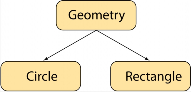
Inheritance allows the programmer to define a class with general properties and behavior and derive one or more specialized subclasses from it that inherit these properties and behavior but also can modify them to add more specialized properties and realize more specialized behavior. We use the terms derived class and base class to refer to the two classes involved when one class is derived from another.
4.7.1 Implementing the class hierarchy
Let’s change our example so that both Circle and Rectangle are derived from such a general class called Geometry. This class will be an abstract class in the sense that it is not intended to be used for creating objects from. Its purpose is to introduce properties and templates for methods that all geometric classes in our project have in common.
class Geometry():
def __init__(self, x = 0.0, y = 0.0):
self.x = x
self.y = y
def computeArea(self):
pass
def computePerimeter(self):
pass
def move(self, deltaX, deltaY):
self.x += deltaX
self.y += deltaY
def __str__(self):
return 'Abstract class Geometry should not be instantiated and derived classes should override this method!'
The constructor of class Geometry looks pretty normal, it just initializes the instance variables that all our geometry objects have in common, namely x and y coordinates to describe their location in our 2D coordinate system. This is followed by the definitions of the methods computeArea(), computePerimeter(), move(…), and __str__() that all geometry objects should support. For move(…), we can already provide an implementation because it is entirely based on the x and y instance variables and works in the same way for all geometry objects. That means the derived classes for Circle and Rectangle will not need to provide their own implementation. In contrast, you cannot compute an area or perimeter in a meaningful way just from the position of the object. Therefore, we used the keyword pass to indicate that we are leaving the body of the computeArea() and computePerimeter() methods intentionally empty. These methods will have to be overridden in the definitions of the derived classes with implementations of their specialized behavior. We could have done the same for __str__() but instead we return a warning message that this class should not have been instantiated.
It is worth mentioning that, in many object-oriented programming languages, the concepts of an abstract class (= a class that cannot be instantiated) and an abstract method (= a method that must be overridden in every subclass that can be instantiated) are built into the language. That means there exist special keywords to declare a class or method to be abstract and then it is impossible to create an object of that class or a subclass of it that does not provide an implementation for the abstract methods. In Python, this has been added on top of the language via a module in the standard library called abc (for abstract base classes). Although we won’t be using it in this course, it is a good idea to check it out and use it if you get involved in larger Python projects. This Abstract Classes page is a good source for learning more.
Here is our new definition for class Circle that is now derived from class Geometry. We also use a few commands at the end to create and use a new Circle object of this class to make sure everything is indeed working as before:
import math
class Circle(Geometry):
def __init__(self, x = 0.0, y = 0.0, radius = 1.0):
super(Circle,self).__init__(x,y)
self.radius = radius
def computeArea(self):
return math.pi * self.radius ** 2
def computePerimeter (self):
return 2 * math.pi * self.radius
def __str__(self):
return 'Circle with coordinates {0}, {1} and radius {2}'.format(self.x, self.y, self.radius)
circle1 = Circle(10, 10, 10)
print(circle1.computeArea())
print(circle1.computePerimeter())
circle1.move(2,2)
print(circle1)
Here are the things we needed to do in the code:
- In line 3, we had to change the header of the class definition to include the name of the base class we are deriving Circle from (‘Geometry’) within the parentheses.
- The constructor of Circle takes the same three parameters as before. However, it only initializes the new instance variable radius in line 7. For initializing the other two variables it calls the constructor of its base class, so the class Geometry, in line 6 with the command “super(Circle,self).__init__(x,y)”. This is saying “call the constructor of the base class of class Circle and pass the values of x and y as parameters to it”. It is typically a good idea to call the constructor of the base class as the first command in the constructor of the derived class so that all general initializations are taken care off.
- Then we provide definitions of computeArea() and computePerimeter() that are specific for circles. These definitions override the “empty” definitions of the Geometry base class. This means whenever we invoke computeArea() or computePerimeter() for an object of class Circle, the code from these specialized definitions will be executed.
- Note that we do not provide any definition for method move(…) in this class definition. That means when move(…) will be invoked for a Circle object, the code from the corresponding definition in its base class Geometry will be executed.
- We do override the __str__() method to produce the same kind of string with information about all instance variables that we had in the previous definition. Note that this function accesses both the instance variables defined in the parent class Geometry as well as the additional one added in the definition of Circle.
The new definition of class Rectangle, now derived from Geometry, looks very much the same as that of Circle if you replace “Circle” with “Rectangle”. Only the implementations of the overridden methods look different, using the versions specific for rectangles.
class Rectangle(Geometry):
def __init__(self, x = 0.0, y = 0.0, width = 1.0, height = 1.0):
super(Rectangle, self).__init__(x,y)
self.width = width
self.height = height
def computeArea(self):
return self.width * self.height
def computePerimeter (self):
return 2 * (self.width + self.height)
def __str__(self):
return 'Rectangle with coordinates {0}, {1}, width {2} and height {3}'.format(self.x, self.y, self.width, self.height )
rectangle1 = Rectangle(15,20,4,5)
print(rectangle1.computeArea())
print(rectangle1.computePerimeter())
rectangle1.move(2,2)
print(rectangle1)
4.7.2 Adding another class to the hierarchy
Overall, the new definitions of Circle and Rectangle have gotten shorter and redundant code like the implementation of move(…) only appears once, namely in the most general class Geometry. Let’s add another class to the hierarchy, a class for axis-aligned Square objects. Of course, you could argue that our class Rectangle is already sufficient to represent such squares. That is correct but we want to illustrate how it would look if you specialize a class already derived from Geometry further and one could well imagine a more complex version of our toy GIS example in which squares would add some other form of specialization. The resulting class hierarchy will then look like in the image below. The new class Square is a derived class of class Rectangle (so Rectangle is its base class) but it is also indirectly derived from class Geometry. Therefore, we say both Geometry and Rectangle are superclasses of Square and Square is a subclass of both these classes. Please note that the way we have been introducing these terms here, the terms base and derived class desribe the relationship between two nodes directly connected by a single arrow in the hierarchy graph, while superclass and subclass are more general and describe the relationship between two classes that are connected via any number of directed arrows in the graph.
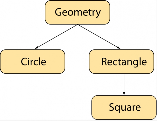
Here is the code for class Square:
class Square(Rectangle):
def __init__(self, x = 0.0, y = 0.0, sideLength = 1.0):
super(Square,self).__init__(x, y, sideLength, sideLength)
def __str__(self):
return 'Square with coordinates {0}, {1} and sideLength {2}'.format(self.x, self.y, self.width )
square1 = Square(5, 5, 8)
print(square1.computeArea())
print(square1.computePerimeter())
square1.move(2,2)
print(square1)
Right, the definition of Square is really short; we only define a new constructor that only takes x and y coordinates and a single sideLength value rather than width and height values. In the constructor we call the constructor of the base class Rectangle and provide sideLength for both the width and height parameters of that constructor. There are no new instance variables to initialize, so this is all that needs to happen in the constructor. Then the only other thing we have to do is override the __str__() method to produce some square-specific output message using self.width for the side length information for the square. (Of course, we could have just as well used self.height here.) The implementations of methods computeArea() and computePerimeter() are inherited from class Rectangle and the implementation of move(…) indirectly from class Geometry.
Now that we have this class hierarchy consisting of one abstract and three instantiable classes, the following code example illustrates the power of polymorphism. Imagine that in our toy GIS we have created a layer consisting of objects of the different geometry types. If we now want to implement a function computeTotalArea(…) that computes the combined area of all the objects in a layer, this can be done like this:
layer = [ circle1, rectangle1, square1, Circle(3,3,9), Square(30, 20, 5) ] def computeTotalArea(geometryLayer): area = 0 for geom in geometryLayer: area += geom.computeArea() return area print(computeTotalArea(layer))
Output: 677.6282702997526
In line 1, you see how we can create a list of objects of the different classes from our hierarchy to represent the layer. We included objects that we already created previously in variables circle1, rectangle1, and square1 but also added another Circle and another Square object that we are creating directly within the square brackets […]. The function computeTotalArea(…) then simply takes the layer list, loops through its elements, and calls computeArea() for each object in the list. The returned area values are added up and returned as the total area.
The code for this is really compact and elegant without any need for if-else to realize some case-distinction based on the geometry type of the given object in variable geom. Let’s further say we would like to add another class to our hierarchy, a class Polygon that – since polygons are neither specialized versions of circles or rectangles – should be derived from the root class Geometry. Since polygons are much more complex than the basic shapes we have been dealing with so far (e.g. when it comes to computing their area), we will not provide a class definition here. But, once we have written the class, we can include polygons in the layer list from the previous example …
layer = [ Polygon(…), circle1, rectangle1, square1, Circle(3,3,9), Square(30, 20, 5) ]
… and the code for computing the total area will immediately work without further changes. All changes required for making this addition are nicely contained within the class definition of Polygon because of the way inheritance and polymorphism are supported in Python.
4.8 Class Attributes and Static Class Functions
In this section we are going to look at two additional concepts that can be part of a class definition, namely class variables/attributes and static class functions. We will start with class attributes even though it is the less important one of these two concepts and won't play a role in the rest of this lesson. Static class functions, on the other hand, will be used in the walkthrough code of this lesson and also will be part of the homework assignment.
We learned in this lesson that for each instance variable defined in a class, each object of that class possesses its own copy so that different objects can have different values for a particular attribute. However, sometimes it can also be useful to have attributes that are defined only once for the class and not for each individual object of the class. For instance, if we want to count how many instances of a class (and its subclasses) have been created while the program is being executed, it would not make sense to use an instance variable with a copy in each object of the class for this. A variable existing at the class level is much better suited for implementing this counter and such variables are called class variables or class attributes. Of course, we could use a global variable for counting the instances but the approach using a class attribute is more elegant as we will see in a moment.
The best way to implement this instance counter idea is to have the code for incrementing the counter variable in the constructor of the class because that means we don’t have to add any other code and it’s guaranteed that the counter will be increased whenever the constructor is invoked to create a new instance. The definition of a class attribute in Python looks like a normal variable assignment but appears inside a class definition outside of any method, typically before the definition of the constructor. Here is what the definition of a class attribute counter for our Geometry class could look like. We are adding the attribute to the root class of our hierarchy so that we can use it to count how many geometric objects have been created in total.
class Geometry():
counter = 0
def __init__(self, x = 0.0, y = 0.0):
self.x = x
self.y = y
Geometry.counter += 1
…
The class attribute is defined in line 2 and the initial value of zero is assigned to it when the class is loaded so before the first object of this class is created. We already included a modified version of the constructor that increases the value of counter by one. Since each constructor defined in our class hierarchy calls the constructor of its base class, the counter class attribute will be increased for every geometry object created. Please note that the main difference between class attributes and instance variables in the class definition is that class attributes don’t use the prefix “self.” but the name of the class instead, so Geometry.counter in this case. Go ahead and modify your class Geometry in this way, while keeping all the rest of the code unchanged.
While instance variables can only be accessed for an object, e.g. using <variable containing the object>.<name of the instance variable>
print(Geometry.counter)
… to get the value currently stored in this new class attribute. Since we have not created any geometry objects since making this change, the output should be 0.
Let’s now create two geometry objects of different types, for instance, a circle and a square:
Circle(10,10,10) Square(5,5,8)
Now run the previous print statement again and you will see that the value of the class variable is now 2. Class variables like this are suitable for storing all information related to the class, so essentially everything that does not describe the state of individual objects of the class.
Class definitions can also contain definitions of functions that are not methods, meaning they are not invoked for a specific object of that class and they do not access the state of a particular object. We will refer to such functions as static class functions. Like class attributes they will be referred to from code by using the name of the class as prefix. Class functions allow for implementing some functionality that is in some way related to the class but not the state of a particular object. They are also useful for providing auxiliary functions for the methods of the class. It is important to note that since static class functions are associated with the class but not an individual object of the class, you cannot directly refer to the instance variables in the body of a static class function like you can in the definitions of methods. However, you can refer to class attributes as you will see in a moment.
A static class function definition can be distinguished from the definition of a method by the lack of the “self” as the first parameter of the function; so it looks like a normal function definition but is located inside a class definition. To give a very simple example of a static class function, let’s add a function called printClassInfo() to class Geometry that simply produces a nice output message for our counter class attribute:
class Geometry():
…
def printClassInfo():
print( "So far, {0} geometric objects have been created".format(Geometry.counter) )
We have included the header of the class definition to illustrate how the definition of the function is embedded into the class definition. You can place the function definition at the end of the class definition, but it doesn’t really matter where you place it, you just have to make sure not to paste the code into the definition of one of the methods. To call the function you simply write:
Geometry.printClassInfo()
The exact output depends on how many objects have been created but it will be the current value of the counter class variable inserted into the text string from the function body.
Go ahead and save your completed geometry script since we'll be using it later in this lesson.
In the program that we will develop in the walkthroughs of this lesson, we will use static class functions that work somewhat similarly to the constructor in that they can create and return new objects of the class but only if certain conditions are met. We will use this idea to create event objects for certain events detected in bus GPS track data. The static functions defined in the different bus event classes (called detect()) will be called with the GPS data and only return an object of the respective event class if the conditions for this kind of bus event are fulfilled. Here is a sketch of a class definition that illustrates this idea:
class SomeEvent():
...
# static class function that creates and returns an object of this class only if certain conditions are satisfied
def detect(data):
... # perform some tests with data provided as parameter
if ...: # if conditions are satisfied, use constructor of SomeEvent to create an object and return that object
return SomeEvent(...)
else: # else the function returns None
return None
# calling the static class function from outside the class definition,
# the returned SomeEvent object will be stored in variable event
event = SomeEvent.detect(...)
if event: # test whether an object has been returned
... # do something with the new SomeEvent object
4.9 Inheritance in GUI Programming
Inheritance also plays an important role in GUI programming. For instance, the widget classes of a GUI library are typically organized in a class hierarchy with some basic class like QWidget towards the top and more specialized widgets like buttons and dialog boxes derived from it. Other parts of the GUI library like the event system are also typically organized hierarchically. Have a quick look at this QT class chart and see how, for instance, the QPushButton is a subclass of QWidget with an intermediate class QButton in between from which also other types of buttons like QCheckbox and QRadioButton are derived. This chart is for version 3 of QT; the chart for version 5 has unfortunately somehow disappeared but the relation between these classes is still the same in QT5.
Let’s think back to the GUI programming sections from Lesson 2: there, we often created widgets, stored them in a variable, and then made changes to the widgets like changing their properties and adding child widgets from the main part of the code. For instance, in the miles-to-kilometers conversion tool from Section 2.5.2.3, we created a QWidget for the main window and then changed its properties and added the child widgets for the other GUI elements like this:
rootWindow = QWidget()
rootWindow.setWindowTitle("Miles to kilometers")
rootWindow.resize(500, 200)
gridLayout = QGridLayout(rootWindow)
labelMiles = QLabel('Distance in miles:')
gridLayout.addWidget(labelMiles, 0, 0)
… and so on. We mainly took this approach because at that point we hadn’t covered the fundamentals of object-oriented programming and inheritance yet and our examples were still rather simple. Typically, what one would rather do is use inheritance to create a new widget class derived from an existing widget class. This new class then implements some specialized behavior compared to its base class and encapsulates everything related to this kind of widget in a single class definition. For instance, for the conversion tool, it makes sense to define a new class that is derived from QWidget like this:
from PyQt5.QtWidgets import QApplication, QWidget, QLabel, QGridLayout, QLineEdit, QPushButton
class ConverterWidget(QWidget):
def __init__(self):
super(ConverterWidget,self).__init__()
self.setWindowTitle("Miles to kilometers")
self.resize(500, 200)
self.gridLayout = QGridLayout(self)
self.labelMiles = QLabel('Distance in miles:')
self.gridLayout.addWidget(self.labelMiles, 0, 0)
self.labelKm = QLabel('Distance in kilometers:')
self.gridLayout.addWidget(self.labelKm, 2, 0)
self.entryMiles = QLineEdit()
self.gridLayout.addWidget(self.entryMiles, 0, 1)
self.entryKm = QLineEdit()
self.gridLayout.addWidget(self.entryKm, 2, 1)
self.convertButton = QPushButton('Convert')
self.gridLayout.addWidget(self.convertButton, 1, 1)
self.convertButton.clicked.connect(self.convert)
def convert(self):
miles = float(self.entryMiles.text())
self.entryKm.setText(str(miles * 1.60934))
app = QApplication([])
converter = ConverterWidget()
converter.show()
app.exec_()
In line 3, we say that our new class ConverterWidget should be derived from the PyQT5 class QWidget, meaning it will inherit all instance variables and methods (like setWindowTitle(…) and resize(…)) from QWidget. In the constructor of our class, we first call the constructor of the base class (line 6) and then set up the GUI of our widget similar to how we did this before from the main part of the code. However, now we store the different child widgets in instance variables (e.g., self.gridLayout) and invoke methods as self.setWindowTitle(…), for instance, because these are now inherited methods of this new class. The convert() event handler function has become a method of our new class and we connect it to the “clicked” signal of the button in line 28 using the prefix “self.” because it is a method of the class we are defining here. The main code of the program following the class definition has become very simple now: we just create an instance of our new class ConverterWidget in variable converter in line 35 and then call its show() method (inherited from QWidget) to make the widget show up on the screen.
As a result of defining a new widget class via inheritance, we now have everything related to our conversion widget nicely encapsulated in the class definition, which also helps in keeping the main code of our script as simple and clean as possible. If we need a conversion widget as part of another project, all we would need to move over to this project is the class definition of ConverterWidget. Another advantage that is not immediately obvious in this toy example is the following: think of situations in which you might need several instances of the widget. In the original version you would have to repeat the code for producing the converter widget. Here you can simply create another instance of the ConverterWidget class by repeating the command from line 35 and store the created widget in a different variable.
4.9.1 Another example involving painting on PyQ5 widgets
Understanding this idea of building reusable GUI components via inheritance is so important that we should look at another example. While doing so, we will also learn how you can actually programmatically draw on a widget to display your own content. What we are going to do is take the classes from our Geometry hierarchy from the previous section and create a widget that actually draws the instances of the classes we have stored in a list to the screen. To make this a bit more interesting, we also want all the objects of the different geometry types to have a “color” attribute that determines in which color the object should be drawn. Before we look at what changes need to be made to the different geometry classes, here is a quick introduction to drawing with PyQt5.
Every widget in QT5 has a method called paintEvent(…) that is called when the widget needs to be drawn (for instance, when its drawn for the first time or when the size of the widget has changed). The only parameter passed to this method is an event object that can be used to get the current dimensions of the content area that we can draw on by calling its rect() method. That means when we want to use a widget for drawing something on it, we derive a new class from the respective widget class and override the paintEvent(…) method with our own implementation that takes care of the drawing. To do the actual drawing, we need to create an object of the class QPainter and then use the drawing methods it provides. Here is a simple example; the details will be explained below:
import sys
from PyQt5 import QtGui, QtWidgets
from PyQt5.QtCore import Qt, QPoint
class MyWidget(QtWidgets.QWidget):
def paintEvent(self, event):
qp = QtGui.QPainter()
qp.begin(self)
qp.setPen(QtGui.QColor(200,0,0))
qp.drawText(20,20, "Text at fixed coordinates")
qp.drawText(event.rect(), Qt.AlignCenter, "Text centered in the drawing area")
qp.setPen(QtGui.QPen(Qt.darkGreen, 4))
qp.drawEllipse(QPoint(50,60),30,30)
qp.setPen(QtGui.QPen(Qt.blue, 2, join = Qt.MiterJoin))
qp.drawRect(20,60,50,80)
qp.end()
app = QtWidgets.QApplication(sys.argv)
window = MyWidget()
window.show()
sys.exit(app.exec_())
When you run this small script, you should see the following window on your screen:
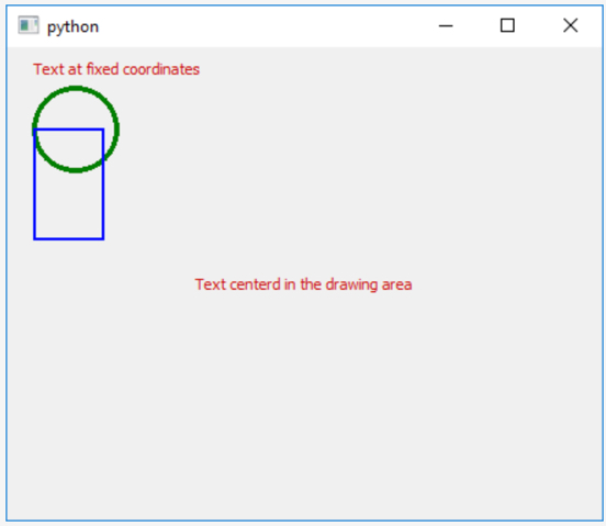
Let’s look at the coarse structure first: we are defining a new class derived from QWidget and only overriding the paintEvent(…) method, meaning in all other aspects this widget will behave like an instance of QWidget. In the main code, we simply create an instance of our new widget class and make it show up on the screen. Now, let’s look at the body of method paintEvent(…): The first thing to note here is that all drawing needs to be preceded by the creation of the QPainter object (line 8) and the call of its begin(…) method using “self” as the parameter standing for the widget object itself because that is what we want to draw on (line 9). To conclude the drawing, we need to call the end() method of the QPainter object (line 19).
Next, let us look at the methods of the QPainter object we are invoking that all start with “draw…”. These are the methods provided by QPainter to draw different kinds of entities like text, circles or ellipses, rectangles, images, etc. We here use the method drawText(…) twice to produce the two different lines of text (lines 12 and 13). The difference between the two calls is that in the first one we use absolute coordinates, so the text will be drawn at pixel coordinates 20, 20 counting from the top left corner of the widget’s content area. The second call takes a rectangle (class QRectF) as the first parameter and then draws the text within this rectangle based on the additional text options given as the second parameter which here says that the text should be centered within the rectangle. This is an example where a class provides several methods with the same name but different parameters, something that is called overloading. If you check out the documentation of QPainter, you will see that most methods come in different versions. Now go ahead and resize the window a bit and see how the text produced by the first call always remains at the same absolute position, while that from the second call always stays centered within the available area.
In line 15, we use the method drawEllipse(…) to produce the circle. There is no special circle drawing method, so we use this one and then provide the same number for the two radii. To draw the rectangle, we use the method drawRect(…) in the version that takes the coordinates of the corner plus width and height values as parameters.
The remaining calls of methods of the QPainter object are there to affect the way the objects are drawn, e.g. their color. Colors inPyQt5 are represented by instances of the class QColor. In line 11, we create a new QColor object by providing values between 0 and 255 for the color’s red, green, and blue values. Since the red value is 200 and both green and blue are zero, the overall color will be the kind of red that the text appears in. QT5 also has a number of predefined colors that we are using in lines 14 (Qt.darkGreen) and 16 (Qt.blue).
QPainter uses objects of class QPen and QBrush to draw the boundary and inside of a shape. In line 11, it is stated that a pen with red color should be used for the following drawing operations. As a result, both text lines appear in red. In line 14, we create a new QPen object to be used by the QPainter and specify that the color should be dark green, and the line width should be 4. This is used for drawing the circle. In line 16, we do the same with color blue and line width 2, and, in addition, we say that sharp corners should be used for the connection between to adjacent line segments of the shape’s border. This is used for drawing the rectangle. We won’t go further into the details of the different pen and brush properties here but the documentation of the QPen and QBrush classes provides some more examples and explanations. In addition, you will see more use cases in the walkthrough in the next section.
4.9.2 Adapting the geometry example
We are now going to revist the geometry example we saved in Section 4.8.
To prepare our geometry classes to be drawn on the screen, we first need to modify their definitions by
- introducing the new “color” instance variable for storing a QColor object,
- defining a method called “paint” for drawing the respective object on a screen. This method will have one parameter called “painter” for passing an object of the QPainter class that can be used for drawing onto the widget.
As an exercise, think about where in the class hierarchy you would need to make changes to address points (1) and (2). Once you have thought about this for a bit, read on.
The new attribute “color” is something that all our geometry classes have in common. Therefore, the best place to introduce it is in the root class Geometry. In all subclasses (Circle, Rectangle, Square), you then only have to adapt the constructor to include an additional keyword parameter for the color. Regarding point (2): As we saw above, drawing a circle or a rectangle requires different methods of the QPainter object to be called with different kinds of parameters specific to the particular geometry type. Therefore, we define the method paint(…) in class Geometry but then override it in the subclasses Circle and Rectangle. For class Square, the way it is based on class Rectangle allows us to directly use the implementation of paint(…) from the Rectangle class, so we do not have to override the method in the definition of Square. Here are the changes made to the four classes.
Class Geometry: as discussed, in class Geometry we introduce the “color” variable, so we need to change the constructor a bit. In addition, we add the method paint(…) but without an implementation. The rest of the definition remains unchanged:
class Geometry:
def __init__(self, x = 0.0, y = 0.0, color = Qt.black):
self.x = x
self.y = y
self.color = color
...
def paint(self, painter):
pass
Classes Circle and Rectangle: for the classes Circle and Rectangle, we adapt the constructors to also include a keyword argument for “color”. The color is directly passed on to the constructor of the base class, while the rest of the constructor remains unchanged. We then provide a definition for method paint(…) that sets up the Pen object to use the right color and then uses the corresponding QPainter method for drawing the object (drawEllipse(…) for class Circle and drawRect(…) for class Rectangle) providing the different instance variables as parameters. The rest of the respective class definitions stay the same:
class Circle (Geometry):
def __init__(self, x = 0.0, y = 0.0, radius = 1.0, color = Qt.black):
super(Circle,self).__init__(x,y,color)
self.radius = radius
...
def paint(self, painter):
painter.setPen(QtGui.QPen(self.color, 2))
painter.drawEllipse(QPoint(self.x, self.y), self.radius, self.radius)
class Rectangle(Geometry):
def __init__(self, x = 0.0, y = 0.0, width = 1.0, height = 1.0, color = Qt.black):
super(Rectangle,self).__init__(x,y, color)
self.width = width
self.height = height
...
def paint(self, painter):
painter.setPen(QtGui.QPen(self.color, 2, join = Qt.MiterJoin))
painter.drawRect(self.x, self.y, self.width, self.height)
Class Square: sor the Square class, we just adapt the constructor to include the color, the rest remains unchanged:
class Square(Rectangle):
def __init__(self, x = 0.0, y = 0.0, sideLength = 1.0, color = Qt.black):
super(Square,self).__init__(x, y, sideLength, sideLength, color)
Now that we have the geometry classes prepared, let us again derive a specialized class GeometryDrawingWidget from QWidget that stores a list of geometry objects and in the paintEvent(…) method sets up a QPainter object for drawing on its content area and then invokes the paint(…) methods for all objects from the list. This is bascially the same thing we did towards the end of Section 4.7.2 but now happens inside the new widget class. The list of objects is supposed to be given as a parameter to the constructor of GeometryDrawingWidget:
import math, sys
from PyQt5 import QtGui, QtWidgets
from PyQt5.QtCore import Qt, QPoint
class GeometryDrawingWidget(QtWidgets.QWidget):
def __init__(self, objects):
super(GeometryDrawingWidget,self).__init__()
self.objectsToDraw = objects
def paintEvent(self, event):
qp = QtGui.QPainter()
qp.begin(self)
for obj in self.objectsToDraw:
obj.paint(qp)
qp.end()
Finally, we create another new class called MyMainWindow that is derived from QMainWindow for the main window containing the drawing widget. The constructor takes the list of objects to be drawn and then creates a new instance of GeometryDrawingWidget passing the object list as a parameter and makes it its central widget in line 6:
class MyMainWindow(QtWidgets.QMainWindow):
def __init__(self, objects):
super(MyMainWindow, self).__init__()
self.resize(300,300)
self.setCentralWidget(GeometryDrawingWidget(objects))
In the main code of the script, we then simply create an instance of MyMainWindow with a predefined list of geometry objects and then call its show() method to make the window appear on the screen:
app = QtWidgets.QApplication(sys.argv) objects = [ Circle(93,83,45, Qt.darkGreen), Rectangle(10,10,80,50, QtGui.QColor(200, 0, 250)), Square(30,70,38, Qt.blue)] mainWindow = MyMainWindow (objects) mainWindow.show() sys.exit(app.exec_())
When you run the program, the produced window should look like in the figure below. While this is not really visible, every time you resize the window, the paintEvent(…) method of GeometryDrawingWidget will be called and the content consisting of the three geometric objects will be redrawn. While in this simple widget, we only use fixed absolute coordinates so that the drawn content is independent of the size of the widget, one could easily implement some logic that would scale the drawing based on the available space.
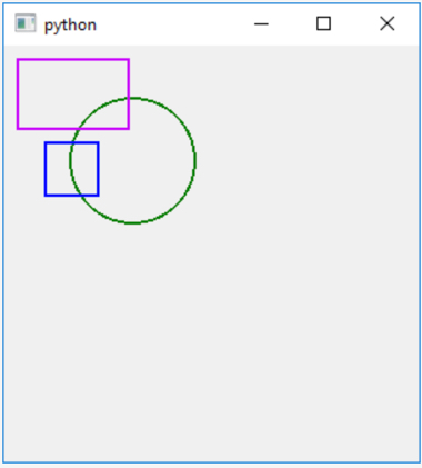
4.10 Walkthrough I: A Bus Track Analyzer for GPS Data of Dublin Buses
It is time to apply what we learned about writing classes, inheritance, and polymorphism in a larger project. In this walkthrough we are going to build an application that processes GPS tracks of buses to detect certain events like a bus being stopped for more than a minute, two buses encountering each other along their routes, etc. Such an application might be used by a public transportation manager to optimize schedules or be warned about irregularities occurring in a real-time tracking data stream. In the walkthrough code, we will be defining classes for real-world objects from the domain like a class Bus, a class Depot, etc. and for abstract concepts like a GPS point with timestamp information and for the events we are looking for. The classes for the different event types we are interested in will be organized into a hierarchy like the geometry classes in section 4.9.
The data we will be using for this project comes from Ireland’s open data portal. The Dublin City Council has published bus GPS data across Dublin City for November 2012 and January 2013 in the form of daily .csv files that list GPS points for active bus vehicles in chronological order with timestamps measured in microseconds since January 1st, 1970. This is a common way of measuring time called Unix or Posix time. GPS measurements for an active vehicle appear in intervals of approximately 20 seconds in the data. The locations are given in WGS84 (EPSG:4326) latitude and longitude coordinates.
We extracted the bus data for 1.5 hours in the late evening of January 30 and morning of January 31, 2013 and cleaned it up a bit, filtering out some outliers and vehicles for which there were only a very small number of GPS points. We manually created a second input file with bounding box coordinates for a few bus depots in Dublin that we will need for detecting certain events and then combined the two input files with some other resources that we will need for this project and the actual source code consisting of several Python .py files. Please download the resulting .zip file and extract it into a new folder.
Have a quick look at the file dublin_bus_data.csv containing the bus GPS points. We are mainly interested in column 1 that contains the time information, column 6 that contains the ID of the bus vehicle, and columns 9 and 10 that contain the latitude and longitude coordinates. We will also use column 2 that contains the number of the line this bus belongs to, but only for information display.
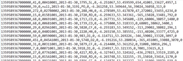
The file dublin_depots.csv contains the bus depot information with columns for the depot name and latitude-longitude pairs for the bottom left and top right corners of the bounding box as a rough approximation of the depot’s actual location and area.
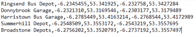
In this walkthrough, we will focus on writing the code for the main classes needed for reading in the data, processing the data and detecting the events, and producing output vector data sets with the bus tracks and detected events. In addition, we will create a QT widget that displays the status of the different buses while the data is being processed. In the following optional part (Sections 4.11 and 4.12), we will further develop this project into a QGIS plugin that includes this widget and shows developing bus trajectories and detected events live as developing layers on the QGIS map canvas.
4.10.1 File and Class Structure of the Project
Since this project involves quite a bit of code, we have tried to cleanly organize it into different class definitions and multiple files. We don’t expect you to type in the code yourself in this walkthrough but rather study the files carefully and use the explanations provided in this text to make sure you understand how everything plays together. Here is an overview on what each of the involved files contains:
core_classes.py – This file contains most of the basic classes for our project that are not derived from other classes.
- class Timepoint: a Timepoint in this project will represent a point in space and time and is therefore defined by latitude and longitude properties which are both instance variables of type float and a time property that is an instance of the class datetime from the datetime module of the Python standard library (that you worked with in homework assignment 3). We will use Timepoints to represent the bus observations from the GPS data as well as events happening at a particular location at a particular time.
- class Bus: the class Bus represents a single vehicle appearing in the GPS data and its GPS points extracted from the input data. It is defined by its vehicle ID, the line it belongs to, and a list of chronologically-ordered Timepoints representing the GPS observation points read from the input data.
- class BusTracker: this class represents the current status of an individual bus vehicle during the analysis and event detection process. A BusTracker object will be maintained for each bus vehicle. It links to the corresponding object of class Bus and, in addition, is used to keep track of whether the vehicle’s status is currently “driving”, “stopped”, or “in depot”, of its current speed estimate, of the last Timepoint that has already been processed for this bus, and of some other information.
- class Observation: in the analysis stage of our program, we will maintain a priority queue (Section 4.2.3) in which we store the next observations for each bus. These observations need to be processed in order of their time of occurrence. The objects we are storing in this queue will be of class Observation that combines the BusTracker for the bus this observation is about, the Timepoint of this observation, and the index of that Timepoint in the list of Timepoints of the bus. Please note that the class has to define its own __lt__(...) method for the < comparison operator to achieve that the Obervation objects in the priority queue will be ordered based on their time attribute of the Timepoint object they contain.
- class Depot: the class Depot is used to represent a single bus depot, simply defined by its name and bounding box which is represented as a 4-tuple of floats as in the original input data in file dublin_depots.csv.
bus_events.py - This file defines the hierarchy of bus events starting with the abstract root class BusEvent from which we derive three more specialized (but still abstract) classes SingleBusEvent, MultipleBusesEvent, and BusDepotEvent. The classes for the events that we are actually trying to detect in the data are derived from these three intermediate classes. The overall bus event hierarchy is depicted in the figure below. We are keeping things somewhat simple here. One could certainly imagine other kinds of events that could be of interest and easily added to this hierarchy.
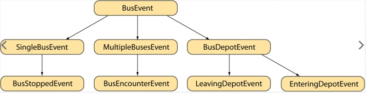
- class BusEvent: each bus event has an associated Timepoint. Therefore, the instance variable for this Timepoint object is already introduced in the abstract root class BusEvent. In addition, each bus event should have a method description() to produce a string with a brief description of the event suitable to be stored in an attribute table of a feature class, and a class function (Section 4.8) called detect(…) that takes an object of class Observation and checks whether the respective event occurs at this observation point and if so, creates and returns one or multiple event objects of that event class. We define templates for both these functions in BusEvent but they need to be overwritten by the derived subclasses.
- class SingleBusEvent: this class is intended as a superclass for all events involving just a single bus, so those that are entirely based on properties of the bus and its GPS data. The class adds an instance variable to refer to the Bus object this event is about.
- class MultipleBusesEvent: this class is the superclass for all bus events that involve two or more buses (like bus encounter events). It adds an instance variable for storing a list of Bus objects, namely those involved in the particular event.
- class BusDepotEvent: all event classes that involve a single bus and a bus depot are supposed to be derived from this intermediate class. It adds instance variables for the involved bus (class Bus) and involved depot (class Depot).
- class BusStoppedEvent: this is the first instantiable class in our hierarchy and it is derived from the SingleBusEvent class because it is only about the properties of an individual bus: when the given Timepoint on the bus doesn’t move more than 3 meters for at least a minute, we consider the bus to be stopped, generate an event of this class, and update the status of the BusTracker for this bus accordingly. This all happens in the function detect(…) that is overwritten in the definition of class BusStoppedEvent. This class adds another instance variable called duration for keeping track of how long the bus remained stopped.
- class BusEncounterEvent: this event derived from class MultipleBusesEvent represents situations in which two buses encounter each other along their routes. The detect(…) function overwritten in the class definition creates an event of this class if the given bus is observed within 20 meters of the last accounted position of another bus while both buses are “driving” (so not stopped and not currently in a depot).
- class LeavingDepotEvent: this class is derived from BusDepotEvent and an event of this class will be generated (again by the overwritten function detect(…)) if the bus still has the status “in depot” but for the given observation now is located outside any depot. The status of the corresponding BusTracker will be changed from “in depot” to “driving”.
- class EnteringDepotEvent: this is the counter part to LeavingDepotEvent for when a bus that still has the status “driving” now for the current observation is located inside one of the depots.
bus_track_analyzer.py – This file contains just a single class definition, the definition of class BusTrackAnalyzer that is our main class for performing the analysis and event detection over the data read in from the two input files. Its constructor takes two input parameters: a dictionary that maps a bus vehicle ID to the corresponding object of class Bus (created from the data from the GPS input file) and a list of Depot objects (created from the data in the depot input file). While its code could also have become the main program for this project, it is advantageous to have this all encapsulated into a class definition with methods for performing a single step of the analysis, resetting the analysis to start from the beginning, and for producing output vector data sets of the bus tracks created and the events detected so far. This way we can use this analyzer differently in different contexts and have full control over when and in which order the individual analysis steps and other actions will be performed. When we turn the project into a QGIS plugin in Section 4.12, we will make use of this by linking the methods of this class to a media player like control GUI with buttons for starting, pausing, and resetting the analysis. We will explain how this main class of the project works in more detail in a moment.
bus_tracker_widget.py – This file also defines just a single class, BusTrackerWidget, which is for visualizing the current status of the buses during the analysis and, therefore, is a bit of an optional component in this project to practice what you learned about drawing on a widget some more in this lesson. A BusTrackerWidget object is directly linked to a BusTrackAnalyzer object that is given to it as a parameter to the constructor. Whenever the content is supposed to be drawn, it accesses the analyzer object and, in particular, the list of BusTracker objects maintained there and depicts the status of the different buses as shown in the image below with each line representing one of the buses:
The class uses the three images from the files status_driving.png, status_indepot.png, and status_stopped.png to show the current status as an icon in the leftmost column of each row. This is followed by a colored circle depicting the vehicles current estimated speed using red for speeds below 15 mph, orange below 25 mph, yellow below 40 mph, and green for speeds larger than 40 mph. Then it displays the bus ID and line information followed by a short text description providing more details on the status like the exact speed estimate or the name of the depot the bus is currently located in. The widget also shows the time of the last processed observation in green at the top. We will discuss how this class has been implemented in more detail later in this section.
main.py – Lastly, this file contains the main program for this project in which we put everything together. Since most of the analysis functionality is implemented in class BusTrackAnalyzer and the detect(…) functions of the different bus event classes, this main program is comparatively compact. It reads in the data from the two input files, creates a BusTrackAnalyzer for the resulting Bus and Depot objects, and sets up a QWidget for a window that hosts an instance of the BusTrackerWidget class. When the main button in this QWidget is pressed, the run method is executed and processes the data step-by-step by iteratively calling the nextStep() method of the analyzer object until all observations have been processed. The method also makes sure that the BusTrackerWidget is repainted after each step so that we can see what is happening during the analysis. Finally, it saves the detected events and bus tracks as vector data sets on the disk.
4.10.2 Implementation Details
Now that you have a broad overview of the classes and files involved, let’s look at the code in more detail. The code is too long to explain every line and there are parts that should be easy to understand with the knowledge you have now and the comments included in the source code, so we will only be picking out the main points. Nevertheless, please make sure to study carefully the class definitions and how they work together, and if something is unclear, please ask on the forums.
4.10.2.1 Reading the Input Data
To study the interplay between the classes and implementation details, let us approach things in the order in which things happen when the main program in main.py is executed. After the main input variables like the paths for the two input files and a dictionary for the indices of the columns in the GPS input file have been defined in lines 15 to 21 of main.py, the first thing that happens is that the data is read in and used to produce objects of classes Bus and Depot for each bus vehicle and depot mentioned in the two input files.
The reading of the input data happens in lines 24 and 25 of main.py.
depotData = Depot.readFromCSV(depotFile) busData = Bus.readFromCSV(busFile, busFileColumnIndices)
Both classes Bus and Depot provide class functions called readFromCSV(...) that given a filename read in the data from the respective input file and produce corresponding objects. For class Depot this happens in lines 112 to 120 of core_classes.py and the return value is a simple list of Depot objects created in line 119 with given name string and 4-tuple of numbers for the bounding box.
def readFromCSV(fileName):
"""reads comma-separated text file with each row representing a depot and returns list of created Depot objects.
The order of columns in the file is expected to match the order of parameters and bounding box elements of the Depot class."""
depots = []
with open(os.path.join(os.path.dirname(__file__), fileName), "r") as depotFile:
csvReader = csv.reader(depotFile, delimiter=',')
for row in csvReader: # go through rows in input file
depots.append(Depot(row[0], (float(row[1]),float(row[2]),float(row[3]),float(row[4])))) # add new Depot object for current row to Depot list
return depots
For class Bus, this happens in lines 20 to 49 of core_classes.py and is slightly more involved. It works somewhat similarly to the code from the rhino/race car project in lesson 4 of GEOG485 in that it uses a dictionary to create Timepoint lists for each individual bus vehicle occurring in the data.
def readFromCSV(fileName, columnIndices):
"""reads comma-separated text file with each row representing a GPS point for a bus with timestamp and returns dictionary mapping
bus id to created Bus objects. The column indices for the important info ('lat', 'lon', 'time', 'busID', 'line') need to be
provided in dictionary columnIndices."""
buses = {}
with open(os.path.join(os.path.dirname(__file__), fileName), "r") as trackFile:
csvReader = csv.reader(trackFile, delimiter=',')
for row in csvReader:
# read required info from current row
busId = row[columnIndices['busId']]
lat = row[columnIndices['lat']]
lon = row[columnIndices['lon']]
time = row[columnIndices['time']]
line = row[columnIndices['line']]
# create datetime object from time; we here assume that time in the csv file is given in microseconds since January 1, 1970
dt = datetime.datetime(1970, 1, 1) + datetime.timedelta(microseconds=int(time))
# create and add new Bus object if this is the first point for this bus id, else take Bus object from the dictionary
if not busId in buses:
bus = Bus(busId, line)
buses[busId] = bus
else:
bus = buses[busId]
# create Timepoint object for this row and add it to the bus's Timepoint list
bus.timepoints.append(Timepoint(dt,float(lat),float(lon)))
return buses # return dictionary with Bus objects created
For each row in the csv file processed by the main for-loop in lines 28 to 47, we extract the content of the cells we are interested in, create a new datetime object based on the timestamp in that row, and then, if no bus with that ID is already contained in the dictionary we are maintaining in variable buses, meaning that this is the first GPS point for this bus ID in the file, we create a new Bus object and put it into the dictionary using the bus ID as the key. Else we keep working with the Bus object we have already stored under that ID in the dictionary. In both cases, we then add a new Timepoint object for the data in that row to the list of Timepoints kept in the Bus object (line 47). The dictionary of Bus objects is returned as the return value of the function. Having all Timepoints for a bus nicely stored as a list inside the corresponding Bus object will make it easy for us to look ahead and back in time to determine things like current estimated speed and whether the bus is stopped or driving at a particular point in time.
4.10.2.2 Setting up the BusTrackAnalyzer
Next, we create the BusTrackAnalyzer object to be used for the event detection in line 28 of main.py providing the bus dictionary and depot list as parameters to the constructor together with a list of class names for the bus event classes that we want the analyzer to detect. This list is defined in line 17 of main.py.
eventClasses = [ LeavingDepotEvent, EnteringDepotEvent, BusStoppedEvent, BusEncounterEvent ] # list of event classes to detect ... # create main BusTrackAnalyzer object analyzer = BusTrackAnalyzer(busData, depotData, eventClasses)
If you look at lines 12 to 21 of bus_track_analyzer.py, you will see that the constructor takes these parameters and stores them in its own instance variables for performing analysis steps later on (lines 16, 17 and 19).
def __init__(self, busData, depotData, eventClasses):
self.allBusTrackers = [] # list of BusTracker objects for all buses currently being processed
self.allEvents = [] # used for storing all Event objects created during an analysis run
self.lastProcessedTimepoint = None # Timepoint of the last Observation that has been processed
self._busData = busData # dictionary mapping bus Id strings to Bus objects with GPS data
self._depotData = depotData # list of Depot objects used for Event detection
self._observationQueue = [] # priority queue of next Observation objects to be processed for each bus
self._eventClasses = eventClasses # list of instantiable subclasses of BusEvent that should be detected
self.reset() # initialize variables for new analysis run
In addition, the constructor sets up some more instance variables that will be needed when the analysis is run: a list of bus trackers (one for each bus) in variable allBusTrackers, a list of events detected in variable allEvents, a variable lastProcessedTimepoint for the Timepoint of the last observation processed, and a list in variable _observationQueue that will serve as the priority queue of Observation objects to be processed next. Then in the last line, we call the method reset() of BusTrackAnalyzer defined in lines 23 to 40 whose purpose is to reset the value of these instance variables to what they need to be before the first analysis step is performed, allowing the analysis to be reset and repeated at any time.
def reset(self):
"""reset current analysis run and reinitialize everything for a new run"""
self.allBusTrackers = []
self.allEvents = []
self.lastProcessedTimepoint = None
self._observationQueue = []
for busId, bus in self._busData.items(): # go through all buses in the data
busTracker = BusTracker(bus) # create new BusTracker object for bus
# set initial BusTracker status to "IN DEPOT" if bus is inside bounding box of one of the depots
isInDepot, depot = Depot.inDepot(bus.timepoints[0].lat, bus.timepoints[0].lon, self._depotData)
if isInDepot:
busTracker.status = BusTracker.STATUS_INDEPOT
busTracker.depot = depot
self.allBusTrackers.append(busTracker) # add new BusTracker to list of all BusTrackers
heapq.heappush(self._observationQueue, Observation(busTracker, 0)) # create Observation for first Timepoint of this bus
# and add to Observation priority queue
The main thing the method does is go through the dictionary with all the Bus objects and, for each, create a new BusTracker object that will be placed in the allBusTrackers list, set the initial status of that BusTracker to STATUS_INDEPOT if the first Timepoint for that bus is inside one of the depots (else the status will be the default value STATUS_DRIVING), and create an Observation object with that BusTracker for the first Timepoint from the Timepoint list of the corresponding bus that will be put into the observation priority queue via the call of the heapq.headpush(…) function (line 40). The image below illustrates how the main instance variables of the BusTrackAnalyzer object may look after this initialization for an imaginary input data set.
The buses with IDs 5, 2145, and 270 are the ones with earliest GPS observations in our imaginary data but there can be more busses that we are not showing in the diagram. We are also not showing all instance variables for each object, just the most important ones. Furthermore, Timepoint objects are shown as simple date + time values in the diagram not as objects of class Timepoint. The arrows indicate which objects the different instance variables contain starting with the _observationQueue, allBusTrackers, and allEvents instance variables of the single BusTrackAnalyzer object that we have.
The Bus objects at the top that contain the GPS data read from the input file will not change anymore and we are not showing here that these are actually maintained in a dictionary. The list of BusTracker objects (one for each Bus object) will also not change anymore but the properties of the individual BusTracker objects in it will change during the analysis. The observation queue list is the one that will change the most during the analysis because it will always contain the Observation objects to be processed ordered by the time point information. The event list is still empty because we have not detected any events yet.
4.10.2.3 Running the Analysis
The method nextStep() defined in lines 47 to 71 of bus_track_analyzer.py is where the main work of running a single step in the analysis, meaning processing a single observation, happens. In addition, the class provides a method isFinished() for checking if the analysis has been completed, meaning there are no more observations to be processed in the observation priority queue. Let us first look at how we are calling nextStep() from our main program:
def run(self):
"""performs only a single analysis step of the BusTrackAnalyzer but starts a timer after each step to call the function again after a
brief delay until the analzzer has finished. Then saves events and bus tracks to GeoPackage output files."""
mainWidget.button.setEnabled(False) # disable button so that it can't be run again
if not analyzer.isFinished(): # if the analyzer hasn't finished yet, perform next step, update widget, and start timer
# to call this function again
analyzer.nextStep()
mainWidget.busTrackerWidget.updateContent()
timer = QTimer()
timer.singleShot(delay, self.run)
else: # when the analyzer has finished write events and bus tracks to new GeoPackage files
analyzer.saveBusTrackPolylineFile("dublin_bus_tracks.gpkg", "GPKG")
analyzer.saveEventPointFile("dublin_bus_events.gpkg", "GPKG")
# reset analyzer and enable button again
analyzer.reset()
mainWidget.button.setEnabled(True)
The method run() in lines 47 to 63 of main.py is called when the “Run” button of our main window for the program is clicked. This connection is done in line 45 of main.py:
self.button.clicked.connect(self.run)
The idea of this method is that unless the analysis has already been completed, it calls nextStep() of the analyzer object to perform the next step (line 53) and then in lines 55 and 56 it starts a QT timer that will invoke run() again once the timer expires. That means run() will be called and executed again and again until all observations have been processed but with small delays between the steps whose length is controlled by variable delay defined in line 21. This gives us some control over how quickly the analysis is run allowing us to observe the changes in the BusTrackerWidget in more detail by increasing the delay value. To make this approach safe, the method first disables the Run button so that the timer is the only way the function can be invoked again.
Now let’s look at the code of nextStep() in more detail (lines 47 to 71 of bus_track_analyzer.py):
def nextStep(self):
"""performs next step by processing Observation at the front of the Observations priority queue"""
observation = heapq.heappop(self._observationQueue) # get Observation that is at front of queue
# go through list of BusEvent subclasses and invoke their detect() method; then collect the events produced
# and add them to the allEvents lists
for evClass in self._eventClasses:
eventsProduced = evClass.detect(observation, self._depotData, self.allBusTrackers) # invoke event detection method
self.allEvents.extend(eventsProduced) # add resulting events to event list
# update BusTracker of Observation that was just processed
observation.busTracker.lastProcessedIndex += 1
observation.busTracker.updateSpeed()
if observation.busTracker.status == BusTracker.STATUS_STOPPED: # if duration of a stopped event has just expired, change status to "DRIVING"
if observation.timepoint.time > observation.busTracker.statusEvent.timepoint.time + observation.busTracker.statusEvent.duration:
observation.busTracker.status = BusTracker.STATUS_DRIVING
observation.busTracker.statusEvent = None
# if this was not the last GPS Timepoint of this bus, create new Observation for the next point and add it to the Observation queue
if observation.timepointIndex < len(observation.busTracker.bus.timepoints) - 1: # not last point
heapq.heappush(self._observationQueue, Observation(observation.busTracker, observation.timepointIndex + 1) )
# update analyzer status
self.lastProcessedTimepoint = observation.timepoint
The code is actually simpler than one might think because the actual event detection is done in the bus event classes. The method does the following things in this order:
- Take next observation from queue: it takes the Observation object at the front of the _observationQueue priority queue out of the queue (line 49). This is the observation with the earliest timestamp that still needs to be processed. Remember that the Observation object consists of a BusTracker object and the observation Timepoint and its index.
- Call detect() function for all event classes: the method then goes through the list of event classes that contains the names of the four event classes making up the bottom level in our bus event hierarchy (see Figure 4.23 from Section 4.10.1) and for each calls the corresponding detect(…) class function (line 54) passing the Observation object as well as the list of depots and the list of all BusTracker objects as parameters, so that the event detection has all the information needed to decide whether an event of this kind is occurring for this observation. The event objects produced and returned as a list from calling detect(…) are then added to the list in allEvent (line 55).
- Update BusTracker: next, the BusTracker object for the current observation is updated to reflect that this Timepoint has been processed and we call its updateSpeed(…) method to compute a new speed estimate based on the current, previous, and next Timepoints for that bus. The code for this method can be found in lines 67 to 81 of core_classes.py and it uses the geopy function great_circle(…) to compute the distance between two WGS84 points. Since our bus event hierarchy does not include an event for when a stopped bus starts to move again, we need some place to change its BusTracker status to STATUS_DRIVING when this happens. This is done in lines 61 to 64 of this method.
- Put next Observation for this bus into queue: unless this observation was for the last Timepoint from the list of Timepoints for that bus, we now generate a new Observation object with the same BusTracker but for the next Timepoint from the Timepoints list and put this Observation into the priority queue (line 68). Since the queue is always kept sorted by observation time, it is guaranteed that all bus observation will be processed in the correct chronological order.
- Update analyzer status: finally, the lastProcessedTimepoint variable of the analyzer itself is updated to always provide the Timepoint of the last Observation processed (line 71).
To illustrate this process, let’s imagine we run the first analysis step for the initial situation from Section 4.10.2.2 with a bus that is not in one of the depots but is nevertheless stopped at the moment. The first Obervation object taken from the queue in step (1) then contains the BusTracker for the bus with ID 2145 and the Timepoint 2013/1/30 23:45:00.
In step(2), we first invoke the detect(…) function of the LeavingDepotEvent class because that is the first class appearing in the list. The code for this function can be found in lines 122 to 140 of bus_events.py.
def detect(observation, depots, activeBusTrackers):
"""process observation and checks whether this event occurs at the given observation. If yes, one or more instances of
this Event class are created and returned as a list."""
producedEvents = [] # initialize list of newly created events to be returned by this function
if observation.busTracker.status == BusTracker.STATUS_INDEPOT:
isInDepot, depot = Depot.inDepot(observation.timepoint.lat, observation.timepoint.lon, depots) # test whether bus is still in a depot
if not isInDepot: # bus not in depot anymore, so leaving depot event will be created and added to result list
event = LeavingDepotEvent(observation.timepoint, observation.busTracker.bus, observation.busTracker.depot)
producedEvents.append(event)
observation.busTracker.status = BusTracker.STATUS_DRIVING # update BusTracker object to reflect detected new status
observation.busTracker.statusEvent = None
observation.busTracker.depot = None
print("Event produced:", str(event))
else:
pass # nothing to do if bus is not in depot
return producedEvents
The first thing tested there is whether or not the current status of the BusTracker is STATUS_INDEPOT which is not the case. Hence, we immediately return from that function with an empty list as the return value. If instead the condition would have been true, the code of this function would have checked whether or not the bus is currenctly still in a depot by calling the Depot.inDepot(...) function (line 128). If that would not be the case, an event object of this class would be created by calling the LeavingDepotEvent(...) constructor (line 130) and the status information in the corresponding BusTracker object would be updated accordingly (lines 132-135). The created LeavingDepotEvent object would be added to the list in variable producedEvents (line 131) that is returned when the end of the function is reached.
Next, this step is repeated with the detect(…) function from EnteringDepotEvent defined in lines 152 to 170 of bus_events.py. The condition that the bus should currently be driving is satisfied, so the code next checks whether or not the current position of the bus given by observation.timepoint.lat and observation.timepoint.lon (line 158) is inside one of the depots by calling the function inDepot(…) defined as part of the class definition of class Depot in lines 104 to 110 of core_classes.py. This is not the case, so again an empty event list is returned.
Next, detect(…) of the class BusStoppedEvent is called. This is most likely the most difficult to understand version of the detect(…) functions and it can be found in lines 35 to 65 of bus_events.py:
def detect(observation, depots, activeBusTrackers):
"""process observation and checks whether this event occurs at the given observation. If yes, one or more instances of
this Event class are created and returned as a list."""
producedEvents = [] # initialize list of newly created events to be returned by this function
if observation.busTracker.status == BusTracker.STATUS_DRIVING:
# look ahead until bus has moved at least 3 meters or the end of the Timepoint list is reached
timeNotMoving = datetime.timedelta(seconds=0) # for keeping track of time the bus hasn't moved more than 3 meters
distance = 0 # for keeping track of distance to original location
c = 1 # counter variable for looking ahead
while distance < 3 and observation.timepointIndex + c < len(observation.busTracker.bus.timepoints):
nextTimepoint = observation.busTracker.bus.timepoints[observation.timepointIndex + c] # next Timepoint while looking ahead
distance = great_circle( (nextTimepoint.lat, nextTimepoint.lon), (observation.timepoint.lat, observation.timepoint.lon) ).m # distance to next Timepoint
if distance < 3: # if still below 3 meters, update timeNotMoving
timeNotMoving = nextTimepoint.time - observation.timepoint.time
c += 1
# check whether bus didn't move for at least 60 seconds and if so generate event
if timeNotMoving.total_seconds() >= 60:
event = BusStoppedEvent(observation.timepoint, observation.busTracker.bus, timeNotMoving) # create stopped event
producedEvents.append(event) # add new event to result list
observation.busTracker.status = BusTracker.STATUS_STOPPED # update BusTracker object to reflect detected stopped status
observation.busTracker.statusEvent = event
print("Event produced: ", str(event))
else:
pass # no stop event will be created while bus status is "IN DEPOT" or "DRIVING"
return producedEvents
The condition is again that the current BusTracker status is “driving” which is satisfied. The code will then run a while-loop that looks at the next Timepoints in the list of Timepoints for this bus until the distance to the current position gets larger than 3 meters. In this case, this only happens for the fifth Timepoint following the current Timepoint. The code then looks at the time difference between these two Timepoints (line 55) and if its more than 60 second, like in this case, creates a new object of class BusStoppedEvent (line 56) using the current Timepoint, Bus object from the BusTracker, and time difference to set the instance variables of the newly created event object. This event object is put into the event list that will be returned by the detect(…) function (line 57). Finally, the status of the BusTracker object involved will be changed to “stopped” (line 58) and we also store the event object inside the BusTracker to be able to change the status back to “driving” when the duration of the event is over (line 59). When we return from the detect(…) function, the produced BusStoppedEvent will be added to the allEvents list of the analyzer (line 55 of bus_track_analyzer.py).
Finally, detect(…) of BusEncounterEvent will be called, the last event class from the list. If you look at lines 83 to 102 of bus_events.py, you will see that a requirement for this event is that the bus is currently “driving”. Since we just changed the status of the BusTracker to “stopped” this is not the case and no events will be generated and returned from this function call. Just to emphasize this again, the details of how the different detect(...) functions work are less important here; the important thing to understand is that we are using the detect(...) functions defined in each of the bottom level bus event classes to test whether or not one (or even multiple) event(s) of that type occurred and if so generate an event object of that class with information describing that event by calling the constructor of the class (e.g., BusStoppedEvent(...)). Each created event object is added to the list that the detect(...) function returns to the calling nextStep(...) function. In the lesson's homework assignment you will have to use a similar approach but within a much less complicated project.
Now steps (3) –(6) are performed with the result that the lastProcessedIndex of the BusTracker is increased by one (to 1), a new estimated speed is computed for it, a new observation is created for bus 2145 and added to the queue, now for time point 2013/1/30 23:45:03. Since the first observation for bus 270 only has a timestamp of 23:45:05, the new Observation is inserted into the queue in second place after the first Observation for the bus with busId 5. Finally, the lastProcessedTimepoint of the analyzer is changed to 2013/1/30 23:45:00. The resulting constellation after this first run of nextStep() is shown in the image below.
We have intentionally placed some print statements inside the bus event classes from bus_events.py whenever a new event of that class is detected and a corresponding object is created. Normally you wouldn’t do that but here we want to keep track of the events produced when running the main program. So test out the program by executing main.py (e.g., from the OSGeo4W shell after running the commands for setting the environment variables as described in Section 4.4.1) and just look at the output produced in the console, while still ignoring the graphical output in the window for a moment.
The produced output will start like this but list quite a few more bus events detected during the analysis:
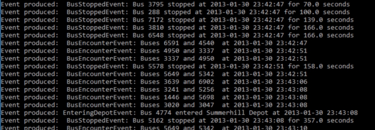
4.10.2.4 Producing the output GPGK files
Remember that we said that the code from main.py will also produce output vector data sets of the bus tracks and events in the end. This happens in lines 57 to 63 of main.py which are only executed when analyzer.isFinished() returns True, so when the analysis has processed all observations:
else: # when the analyzer has finished write events and bus tracks to new GeoPackage files
analyzer.saveBusTrackPolylineFile("dublin_bus_tracks.gpkg", "GPKG")
analyzer.saveEventPointFile("dublin_bus_events.gpkg", "GPKG")
# reset analyzer and enable button again
analyzer.reset()
mainWidget.button.setEnabled(True)
This code assumes that the QGIS environment has already been set up which happens in lines 69 to 73 of main.py; this code should look familiar from Section 4.5.3. The code for creating the output files can be found in the two methods saveBusTrackPolylineFile(…) and saveEventPointFile(…) of BusTrackAnalyzer in lines 73 to 114 of bus_track_analyzer.py.
def saveBusTrackPolylineFile(self, filename, fileFormat):
"""save event list as a WGS84 point vector dataset using qgis under the provided filename and using the given format. It is
expected that qgis has been initalized before calling this method"""
# create layer for polylines in EPSG:4326 and an integer field BUS_ID for storing the bus id for each track
layer = qgis.core.QgsVectorLayer('LineString?crs=EPSG:4326&field=BUS_ID:integer', 'tracks' , 'memory')
prov = layer.dataProvider()
# create polyline features
features = []
for busId, bus in self._busData.items():
# use list comprehension to produce list of QgsPoinXY objects from bus's Timepoints
points = [ qgis.core.QgsPointXY(tp.lon,tp.lat) for tp in bus.timepoints ]
feat = qgis.core.QgsFeature()
lineGeometry = qgis.core.QgsGeometry.fromPolylineXY(points)
feat.setGeometry(lineGeometry)
feat.setAttributes([int(busId)])
features.append(feat)
# add features to layer and write layer to file
prov.addFeatures(features)
qgis.core.QgsVectorFileWriter.writeAsVectorFormat( layer, filename, "utf-8", layer.crs(), fileFormat)
saveBusTrackPolylineFile(…) creates a list of QgsPointXY objects from the Timepoints of each Bus object (line 105) and then creates a Polyline geometry from it (line 107) which is further turned into a feature with an attribute for the ID of the bus, and then added to the created layer in line 113. Finally, the layer is written to a new file using the name and format given as parameter to the function. We here use the GeoPackage format “GPKG” but this can easily be changed in main.py to produce, for instance, a shapefile instead.
def saveEventPointFile(self, filename, fileFormat):
"""save event list as a WGS84 point vector dataset using qgis under the provided filename and using the given format. It is
expected that qgis has been initalized before calling this method"""
# create layer for points in EPSG:4326 and with two string fields called TYPE and INFO
layer = qgis.core.QgsVectorLayer('Point?crs=EPSG:4326&field=TYPE:string(50)&field=INFO:string(255)', 'events' , 'memory')
prov = layer.dataProvider()
# create point features for all events from self.allEvents and use their Event class name
# and string provided by description() method for the TYPE and INFO attribute columns
features = []
for event in self.allEvents:
p = qgis.core.QgsPointXY(event.timepoint.lon, event.timepoint.lat)
feat = qgis.core.QgsFeature()
feat.setGeometry(qgis.core.QgsGeometry.fromPointXY(p))
feat.setAttributes([type(event).__name__, event.description()])
features.append(feat)
# add features to layer and write layer to file
prov.addFeatures(features)
qgis.core.QgsVectorFileWriter.writeAsVectorFormat( layer, filename, "utf-8", layer.crs(), fileFormat)
saveEventPointFile(…) works in the same way but produces QgsPointXY point features with the attribute fields TYPE and INFO for each event in the allEvents list. The TYPE field will contain the name of the event class this event is from, and the INFO field will contain the short description produced by calling the description() method of the event. Notice this just needs a single line (line 87) because of our event class hierarchy and polymorphism. When opening the two produced files in QGIS, adding a basemap, and adapting the symbology a bit, the result looks like this:
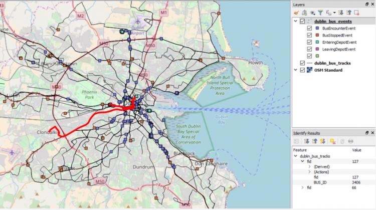
We hope the way this program works got clear from this explanation with (a) the BusTrackAnalyzer being the central class for running the event detection in a step-wise fashion, (b) the Observation objects maintained in a priority queue being used to process the GPS observation in chronological order, (c) the BusTracker objects being used to keep track of the current status of a bus during the analysis, and (d) the different bus event classes all providing their own function to detect whether or not an event of that type has occurred. The program is definitely quite complex but this is the last lesson so it is getting time to see some larger projects and learn to read the source code. As the final step, let's look at the BusTrackerWidget class that provides a visualization of event detection while the analysis process is running.
4.10.2.5 The Bus Tracker Widget for visualizing the analysis process
As we explained before, we also wanted to set up a QT widget that shows the status of each bus tracker while the data is being processed and we implemented the class BusTrackerWidget in bus_tracker_widget.py derived from QWidget for this purpose. In lines 30 to 44 of main.py we are creating the main window for this program and in line 41 we add an instance of BusTrackerWidget to the QScrollArea in the center of that window:
class MainWidget(QWidget):
"""main window for this application containing a button to start the analysis and a scroll area for the BusTrackerWidget"""
def __init__(self, analyzer):
super(MainWidget,self).__init__()
self.resize(300,500)
grid = QGridLayout(self)
self.button = QPushButton("Run")
grid.addWidget(self.button,0,0)
self.busTrackerWidget = BusTrackerWidget(analyzer) # place BusTrackerWidget for our BusTrackAnalyzer in scroll area
scroll = QScrollArea()
scroll.setWidgetResizable(True)
scroll.setWidget(self.busTrackerWidget)
grid.addWidget(scroll, 1, 0)
self.button.clicked.connect(self.run) # when button is clicked call run() function
We are embedding the widget in a QScrollArea to make sure that vertical and horizontal scrollbars will automatically appear when the content becomes too large to be displayed. For this to work, we only have to set the minimum width and height properties of the BusTrackerWidget object accordingly. Please note that in line 53 of main.py we are calling the method updateContent() of BusTrackerWidget so that the widget and its content will be repainted whenever another analysis step has been performed.
Looking at the definition of class BusTrackerWidget in bus_tracker_widget.py, the important things happen in its paintEvent(…) method in lines 24 to 85. Remember that this is the method that will be called whenever QT creates a paint event for this widget, so not only when we force this by calling the repaint() method but also when the parent widget has been resized, for example.
def paintEvent(self, event):
"""draws content with bus status information"""
# set minimum dimensions basd on number of buses
self.setMinimumHeight(len(self.analyzer.allBusTrackers) * 23 + 50)
self.setMinimumWidth(425)
# create QPainter and start drawing
qp = QtGui.QPainter()
qp.begin(self)
normalFont = qp.font()
boldFont = qp.font()
boldFont.setBold(True)
# draw time of last processed Timepoint at the top
qp.setPen(Qt.darkGreen)
qp.setFont(boldFont)
if self.analyzer.lastProcessedTimepoint:
qp.drawText(5,10,"Time: {0}".format(self.analyzer.lastProcessedTimepoint.time))
qp.setPen(Qt.black)
…
The first thing that happens in this code is that we set the minimum height property of our widget based on the number of BusTracker objects that we need to provide status information for (line 27). For the minimum width, we can instead use a fixed value that is large enough to display the rows. Next, we create the QPainter object needed for drawing (line 31 and 32) and draw the time of the last Timepoint processed by the analyzer to the top of the window (line 42) unless its value is still None.
# loop through all BusTrackers in the BusTrackAnalyzer
for index, tracker in enumerate(self.analyzer.allBusTrackers):
...
In the main for-loop starting in line 46, we go through the list of BusTracker objects in the associated BusTrackAnalyzer object and produce one row for each of them. All drawing operations in the loop body compute the y coordinate as the product of the index of the current BusTracker in the list available in variable index and the constant 23 for the height of a single row (e.g., 20 +23 * index in line 49 for drawing the bus status icon).
# draw icon reflecting bus status
qp.drawPixmap(5,20 + 23 * index,self._busIcons[tracker.status])
# draw speed circles
color = Qt.transparent
if tracker.speedEstimate:
if tracker.speedEstimate < 15:
color = Qt.red
elif tracker.speedEstimate < 25:
color = QtGui.QColor(244, 176, 66)
elif tracker.speedEstimate < 40:
color = Qt.yellow
else:
color = Qt.green
qp.setBrush(color)
qp.drawEllipse(80, 23 + 23 * index, 7, 7)
…
The bus status icon is drawn in line 49 using the drawPixmap(…) method with the QPixmap icon from the _busIcons dictionary for the given status of the bus tracker. Next, the small colored circle for the speed has to be drawn which happens in line 53. The color is determined by the if-elif construct in lines 53 to 61.
# draw bus id and line text
qp.setFont(boldFont)
qp.drawText(100, 32 + 23 * index, tracker.bus.busId + " [line "+tracker.bus.line+"]")
# draw status and speed text
qp.setFont(normalFont)
statusText = "currently " + tracker.status
if tracker.status == BusTracker.STATUS_INDEPOT:
statusText += " " + tracker.depot.name
elif tracker.status == BusTracker.STATUS_DRIVING:
if not tracker.speedEstimate:
speedText = "???"
else:
speedText = "{0:.2f} mph".format(tracker.speedEstimate)
statusText += " with " + speedText
qp.drawText(200, 32 + 23 * index, statusText )
Next the bus ID and bus line number are drawn (line 66 and 67). This is followed by the code for creating the status information that contains some case distinctions to construct the string that should be displayed in line 81 in variable statusText based on the current status of the bus.
Now run the program, make the main window as large as possible and observe how the status information in the bus tracker widget is constantly updated like in the brief video below. Keep in mind that you can change the speed this all runs in by increasing the value of variable delay defined in line 21 of main.py. Refresher for running python scripts from the OSGeo4W Shell, you can use python-qgis-ltr, so e.g.
python-qgis-ltr main.py
The video has been recorded with a value of 5. [NOTE: This video (:58) does NOT contain sound.]
After developing the Bus Track Analyzer code as a standalone QGIS based application, we will now turn to the (optional) topic of creating QGIS plugins and how our analyzer code can be turned into a plugin that, as an extension, displays the bus trajectories and detected event live on the QGIS map canvas while the anaylsis is performed.
4.11 Optional: Writing QGIS Plugins
In this section and the next, we are going to demonstrate how to create plugins for QGIS and then turn the Bus Track Analyzer code from the previous walkthrough into a plugin that adds new layers to the current QGIS project and displays the analysis progress live on the map canvas. However, if this lesson has been your first contact with writing classes and your head is swimming a bit with all the new concepts introduced or you are simply running out of time, we suggest that you just briefly skim through these sections and then watch the video from Section 4.12.7 showing the final Bus Track Analyzer for QGIS plugin. While creating a QGIS plugin yourself is one option that would give you full over&above points in this lesson's homework assignment, the content of these two sections is not required for the assignment and the quiz. You can always come back to these sections if you have time left at the end of the lesson or after the end of the class.
In Section 4.5, you already got an idea of how to write Python code that uses the qgis package, and we also made use of this in the walkthrough from the previous section to produce the final output data sets. In this section, we will teach you how to create plugins for QGIS that show up in the plugin manager and can be integrated into the main QGIS GUI.
Instead of programming QGIS plugins from scratch, we will use the Plugin Builder 3 plugin to create the main files needed for us, and then we will modify and complement these to implement the functionality of our plugin. In this section, we will show you the general workflow of creating a plugin using a simple “Random number generator” plugin with only very little actual functionality. In the walkthrough that follows in the next section, we will then apply this approach to create a plugin version of our Bus Track Analyzer tool from the first walkthrough of the lesson.
4.11.1 Creating a Plugin Template with Plugin Builder 3
The plugin builder 3 plugin should already be installed in your QGIS version. If not, please go back to Section 4.4.1 and follow the installation instructions there. Now run the plugin by going Plugins -> Plugin Builder in the main menu.
To create a template for your plugin, you have to work through the dialog boxes of Plugin Builder and fill out the information there. Clicking the “Help” button will open a local .html page with detailed information on the purpose and meaning of the different fields. We fill out the first page as shown in the figure below. Here is a brief overview:
- Class name: this is the name of the main class for our plugin. It needs to be a valid Python class name.
- Plugin name: this is the name of the plugin in readable form. In contrast to the class name, it can contain spaces and other special characters.
- Description: a short description of what the plugin is for.
- Module name: the name of the .py file that will contain the main class for your plugin. Typically, the class name written with underscores rather than in CamelCase is used here.
- Version number & Minimum QGIS version: these are used to specify a version number for your plugin and the minimum QGIS version required to run it.
- Author/Company & Email address: here you provide information about the author of the plugin that will be used to create the copyright information at the beginning of the different files. We have no intentation of publishing this plugin, so we just use “489” here.
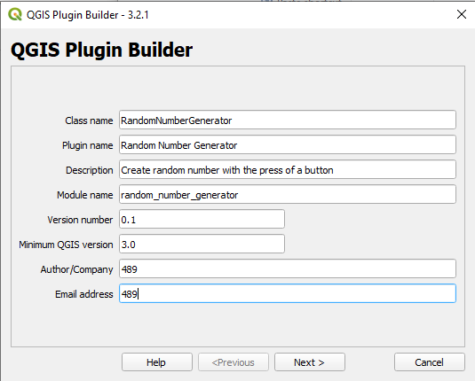
On the next page, you can enter a longer description of your plugin. Since this is just a toy example, we don’t bother with this here and leave the text as it is.
On the next page, you can choose between different kinds of templates for your plugin, e.g. a simple dialog box or a dock widget, meaning an actual panel that can be docked and moved inside the QGIS GUI like the other panels, e.g. the Layers panel. We here will go with the dialog option. In the next section, we will then use the dock widget option. With the “Text for the menu item” option, we specify which text should show up in the menu for our plugin in the main menu bar. With the “Menu” option we pick in which menu of the menu bar this entry should be located. We will fill out this page as shown below:
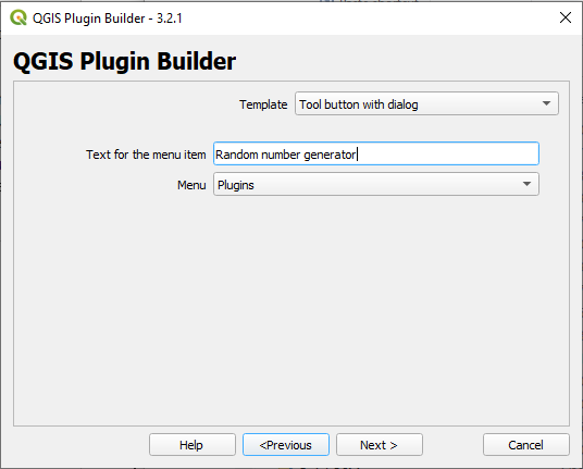
The checkboxes on the next page allow for determining which files Plugin Builder is going to create. It’s ok to leave all options checked.
The next page is specifying information that is relevant if you plan to publish your plugin, e.g. on Github. Since we are not planning this, we just leave the page unchanged.
On the last page, we can determine in which folder the new folder with the files for our plugin will be created. By default this is the default plugin folder of our QGIS installation, meaning the plugin will immediately be listed in QGIS when we start it next. If, instead of the path, you just see a dot (.), please browse to the plugins folder yourself, replacing the part directly after "C:/Users/" with your Windows user name. It is possible that the “AppData” folder in your user’s home directory is not visible in which case you will have to change your settings to show hidden files.
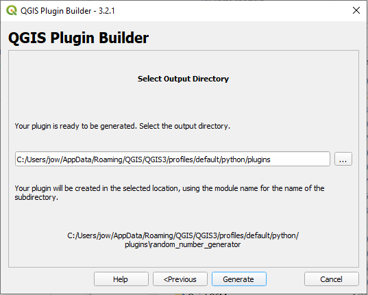
We now click the “Generate” button and Plugin Builder will then create the folder and different files for our plugin. It's possible that you will get a warning message that about Plugin Builder not being able to compile the resources.qrc file; that's ok, we will take care of that in a moment. Plugin Builder will now show us a summary page like in the figure below with some valuable information about where the plugin has been created and what the next steps should be. Even though we won’t be following these exactly, it’s a good idea to take a screenshot of this information or note down where the folder for our plugin is located. You may also want to add the plugins folder under “Quick access” in your Windows File Explorer since we will need to access it quite a lot in the remainder of this lesson.
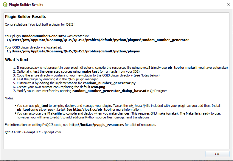
If we now open the new folder “random_number_generator” in the QGIS default plugin folder, you will see the following file structure:
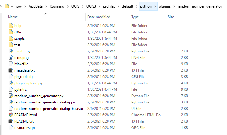
In this introduction to QGIS plugin development, we won’t go into the details of features like internationalization and test code generation, so you can ignore the different subfolders and also some of the files in the main folder. The important files are:
- random_number_generator.py: this file defines the main class RandomNumberGenerator for our plugin. If you look at the code that Plugin Builder 3 generated for this class, you will see that this class has to define a number of methods to interact with QGIS and its plugin interface. One central method is the method run() that in this case here shows our dialog box stored in instance variable self.dlg. If we wanted some code to be executed only if the dialog box is accepted (e.g. closed with the Ok button), then we would put that code here after the “if result:” line.
- random_number_generator_dialog.py: this is the class that defines the main GUI widget for our plugin derived from QDialog. We will talk about this class in more detail in a moment because this is the class that we are going to modify to implement what needs to happen when the user interacts with the GUI of our plugin.
- random_number_generator_dialog_base.ui: this is the class in which the GUI for our dialog box is defined. We will modify it in QT Designer in a moment to adapt the GUI for our purposes.
- __init__.py: A file with this name needs to be contained in the main folder of each plugin and it lets QGIS know about the plugin. QGIS calls the classFactory(…) function defined in this file to create an object of the main class of the plugin (class RandomNumberGenerator in this case).
- metadata.txt: this file contains most of the info about our plugin that we entered into Plugin Builder.
When you now restart QGIS and open the plugin manager under Plugins -> Manage and Install Plugins… , the Random Number Generator plugin should appear in the list of installed plugins but it still needs to be activated. However, if we try to activate it now, we will get an error message that no module called “randomnumbergenerator.resources” can be found. This is a file that we have to generate ourselves by compiling the file called resources.qrc located in our plugin folder with the pyrcc5 tool. The resources file contains information about all additional GUI related resources needed for our plugin, like additional icons for example.
Usually, you would edit the .qrc file first, e.g. in QT Designer, and then compile it. But we don’t need any additional resources for this project, so we just compile it directly with the following command in the OSGeo4W shell after first moving to our plugin folder with the cd command. (The screenshot below contains some commands that were needed in earlier versions of OSGeo4W; you will most likely only need the cd and pyrcc5 commands shown at the bottom.)
pyrcc5 resources.qrc –o resources.py
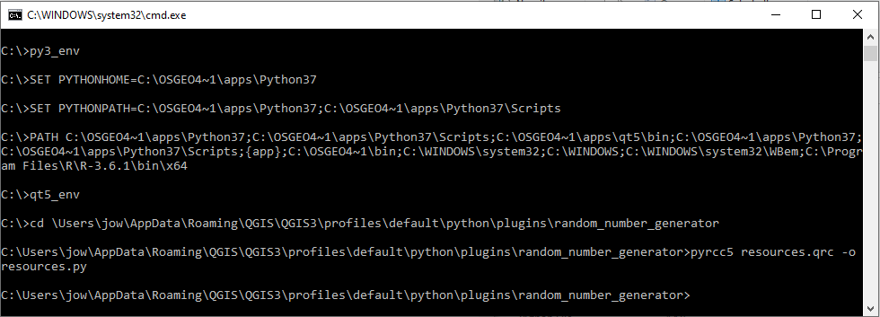
After running this command, we can now activate the plugin by clicking on the checkbox:
There will now be a submenu called “Random Number Generator” with an entry with the same name in the Plugins menu:
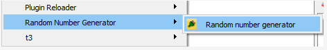
In addition, a toolbar with a single button has been added for our plugin to the toolbar section at the top. Since we didn’t make any changes, the default button  is used. Either clicking the menu entry or the button will open the dialog box for our plugin:
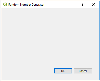
Currently, the dialog box only contains the default elements, namely two buttons for accepting and rejecting the dialog. We are now going to change the GUI of the dialog box and add the random number generation functionality.
4.11.2 Modifying the Plugin GUI and Adding Functionality
The file random_number_generator_dialog.py defines the class RandomNumberGeneratorDialog derived from QDialog. This is the widget class for our dialog box. The GUI itself is defined in the .ui file random_number_generator_dialog_base.ui. In contrast to first compiling the .ui file into a Python .py file and then using the Python code resulting from this to set up the GUI, this class uses the previously briefly mentioned approach of directly reading in the .ui file. That means to change the GUI, all we have to do is modify the .ui file in QT Designer, no compilation needed.
We open random_number_generator_dialog_base.ui with QT Designer and make the following small changes:
- We delete the button box with the Ok and cancel buttons.
- The layout of the dialog box is changed to a vertical layout.
- We add a push button and a label to the dialog box with vertical spacers in between.
- The button text is set to “Press here to generate random number between 1 and 100”.
- The label text is set to “The number is:” and its horizontal alignment property is changed to be horizontally centered.
The image below shows the produced layout in QT Designer.
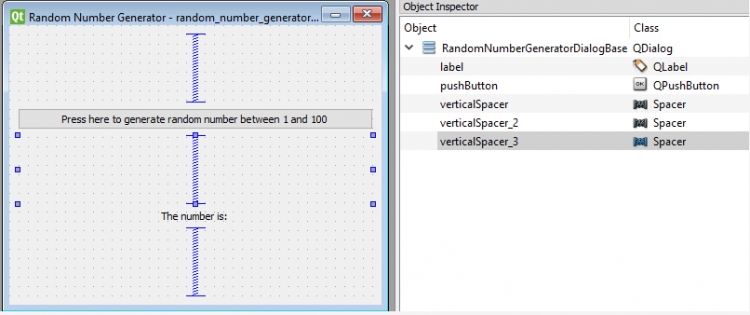
After saving the form, we want to see if we now get the new version of the GUI in QGIS as well. However, for this to happen, the plugin needs to be reloaded. For this, we use the Plugin Reloader plugin that we also installed at the beginning of the lesson. We pick the Plugins -> Plugin Reloader -> Configure option. Then we pick our random_number_generator plugin from the list and press OK.
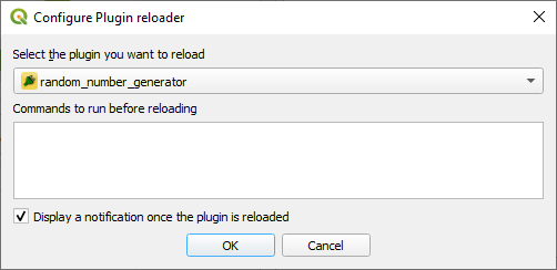
Now we just have to go Plugins -> Plugin Reloader -> Reload: random_number_generator, whenever we want to reload the plugin after making some changes. After doing so and starting our plugin again, it should show up like this in QGIS:
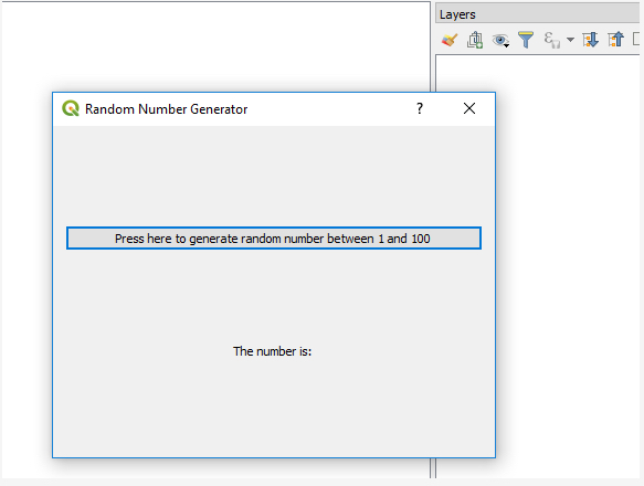
Now we just have to implement the functionality for our plugin, which for this toy example is extremely simple. We just need to write some code for rolling a random number between 1 and 100 and updating the text of the label accordingly when the button is pressed. We implement this in the definition of our class RandomNumberGeneratorDialog in file random_number_generator_dialog.py. The changes we make are the following:
- In the line where the os module is imported, we also import the random module from the Python standard library.
- We add a new method to the class definition with the event handler code:
def generateNewNumber(self): r = random.randint(1,100) self.label.setText("The number is: " + str(r)) - Finally, we connect the button to this new method by adding the following line at the end of the __init__() method:
self.pushButton.clicked.connect(self.generateNewNumber)
Below is the entire code part of random_number_generator_dialog.py after making these changes:
import os, random
from PyQt5 import uic
from PyQt5 import QtWidgets
FORM_CLASS, _ = uic.loadUiType(os.path.join( os.path.dirname(__file__), 'random_number_generator_dialog_base.ui'))
class RandomNumberGeneratorDialog(QtWidgets.QDialog, FORM_CLASS):
def __init__(self, parent=None):
"""Constructor."""
super(RandomNumberGeneratorDialog, self).__init__(parent)
# Set up the user interface from Designer.
# After setupUI you can access any designer object by doing
# self.<objectname>, and you can use autoconnect slots - see
# http://qt-project.org/doc/qt-4.8/designer-using-a-ui-file.html
# #widgets-and-dialogs-with-auto-connect
self.setupUi(self)
self.pushButton.clicked.connect(self.generateNewNumber)
def generateNewNumber(self):
r = random.randint(1,100)
self.label.setText("The number is: " + str(r))
Now the only thing we have to do is reload the plugin again in QGIS, and when we then start the plugin one more time, the button should work and allow us to create random numbers. Please note that the dialog box is opened non-modally from our main plugin class so that you can keep the dialog box open in the background while still interacting with the rest of the QGIS GUI.
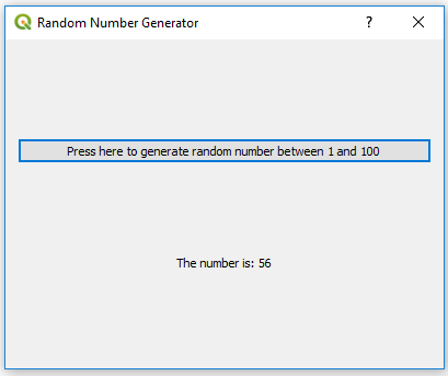
In this small example, all code changes needed were about wiring up the GUI of the dialog box. In such cases, modifying the file with the class definition for the main widget can be sufficient. In the next section, we will implement a plugin that is significantly more complex and interacts with QGIS in more sophisticated ways, e.g., by adding new layers to the currently open project and continuously updating the content of these layers. However, the general approach is the same in that we are mainly going to modify the .ui file and the file with the main widget class from the template files created by Plugin Builder 3. If you want to learn more about QGIS plugin development and the role the other files play, the official documentation is a good starting point.
4.12 Optional: Turning the Bus Event Analyzer into a QGIS Plugin
As said at the beginning of Section 4.11, this section about turning the Bus Track Analyzer code into a plugin that adds new layers to the current QGIS project and displays the analysis progress live on the map canvas can be considered optional. Feel free to just briefly skim through it and then watch the video from Section 4.12.7 showing the final Bus Track Analyzer for QGIS plugin. While creating a QGIS plugin yourself is one option that would give you full over&above points in this lesson's homework assignment, the content of these two sections is not required for the assignment and the quiz. You can always come back to this section if you have time left at the end of this lesson or after the end of the class.
Now that you know how to create plugins for QGIS, let us apply this new knowledge to create a QGIS plugin version of our bus event analyzer from Section 4.10. We will call this plugin “Bus Track Analyzer for QGIS”. The process for this will be roughly as follows:
- Set up a new plugin with Plugin Builder using the Tool “button with dock widget” template
- Copy all the needed files from the project into the plugin folder
- Adapt the default GUI for the dock widget with QT Designer
- Make some smaller modifications to the project files including changes to class BusTrackAnalyzer to define QT signals that we can connect to
- Adapt the code in the dock widget class definition to wire up the GUI and to implement a modified version of the functionality we had in the main program in main.py of the Bus Track Analyzer project
- Implement and integrate a new class QGISEventAndTrackLayerCreator that will be responsible for showing the bus tracks and events detected so far in the QGIS main map window during the analysis
4.12.1 Create Template with Plugin Builder
To create a folder with a template version for this plugin, please follow the steps below.
- Run the Plugin Builder plugin and fill out the first page as follows before clicking “Next >”:
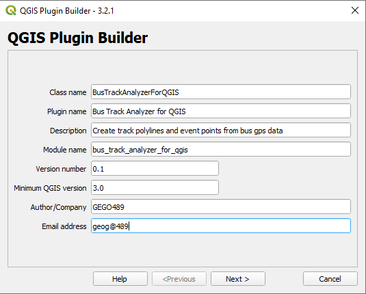 Figure 4.40 First Plugin Builder dialog page with information about the new plugin
 - Just click “Next >” again as we will skip the description part and then on the next page pick the “Tool button with dock widget” template at the top and fill out the rest of the information as shown below before pressing “Next >” again.
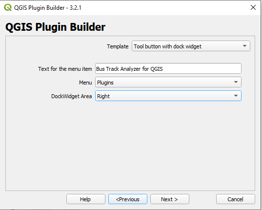 Figure 4.41 Picking the "Tool button with dock widget" template in Plugin Builder
 - We will keep the default settings for the following setup pages, so just keep pressing “Next >” until you arrive at the last page where the button is called “Generate” instead. Take a look at the paths where Plugin Builder is going to create the folder for the new plugin. It might be a good idea to copy the path to somewhere from which you can retrieve it at any time. Now click on “Generate” and the folder for the plugin will be created.
- If you now navigate to the plugins folder from the previous step, it will contain a new folder called “bus_track_analyzer_for_qgis”. Enter that folder and check out the files that have been created. The content should look like this:
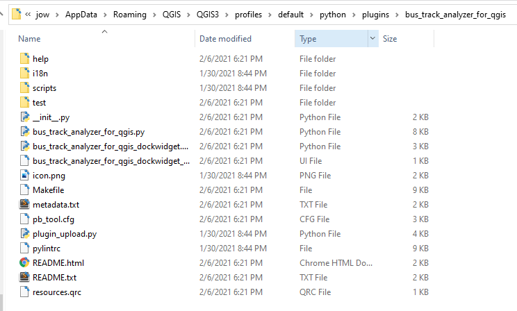 Figure 4.42 Newly created plugin folder with files for our plugin
 - Please close QGIS for a moment. We still need to compile the file resources.qrc into a Python .py file with the help of pyrcc5 as we did in Section 4.11. For this, run OSGeo4W.bat from your OSGeo4W/QGIS installation and, in the shell that opens up, navigate to the folder containing your plugin, e.g. type in the following command but adapt the path to match the path from steps 3 and 4:
cd C:\Users\xyz\AppData\roaming\QGIS\QGIS3\profiles\default\python\plugins\bus_track_analyzer_for_qgis
- Finally, compile the file with the command below. There should now be a file called resources.py in your plugin folder.
pyrcc5 resources.qrc –o resources.py
- You can now restart QGIS and open the plugin manager where “Bus Track Analyzer for QGIS” should now appear in the list of installed plugins. Enable it and then check the Plugins menu to make sure there is now an entry “Bus Track Analyzer for QGIS” there. Start the plugin and a rather empty dock widget will appear in the right part of the QGIS window. Try moving this dock widget around. You will see that you can move it to the other areas of the main QGIS window or completely undock it and have it as an independent window on the screen.
4.12.2 Copy Files into Plugin Folder
For the next steps, it’s best if you again close QGIS for a bit. In case you made any changes to the files during the bus tracking project in Section 4.10, it would be best if you re-download them from here. Then copy the following files from the Section 4.10 project folder (if you didn't edit anything) or the fresh download into the folder for the Bus Tracker plugin:
bus_events.py bus_track_analyzer.py bus_tracker_widget.py core_classes.py dublin_bus_data.csv dublin_depots.csv status_driving.png status_indepot.png status_stopped.png
Please note that we are intentionally not including main.py. Also, it wouldn’t really be necessary to include the input data sets (csv files), but there is also no harm in doing so, and it means that we have everything needed to create and run the plugin together in the same folder.
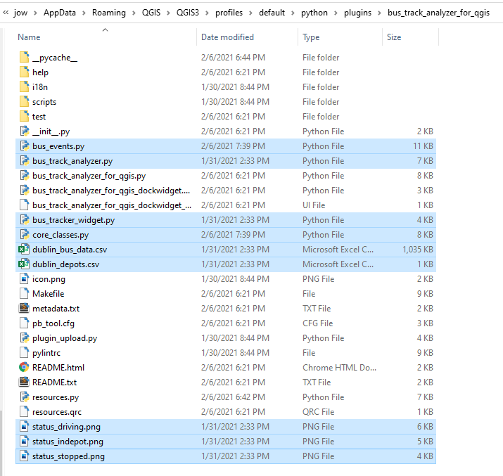
4.12.3 Adapt the GUI with QT Designer
The GUI we will be using for our dock widget is shown in the image below. It has an area at the top where the user can select the GPS and depot input files and a button “Read and init” for reading in the data from the selected files. The central area contains a QScrollArea widget that will host our BusTrackerWidget in the same way as we had it embedded into the main window in the original project. In the area at the bottom, we have the controls for running the analysis consisting of three buttons “Stop and reset”, “Pause”, and “Start” and a QSlider widget for setting the delay between consecutive analysis steps. The image also shows the object names of the important GUI elements that will become instance variables of class BusTrackAnalyzerForQGISDockWidget that we can access and connect to.
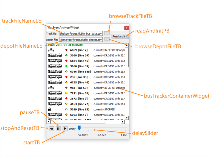
If you look at the files in the folder for our plugin, you will see that Plugin Builder has created a file called bus_track_analyzer_for_qgis_dockwidget.py. This file contains the definition of class BusTrackAnalyzerForQGISDockWidget derived from QDockWidget with the GUI for our plugin. The class itself directly reads the GUI specification from the file bus_track_analyzer_for_qgis_dockwidget_base.ui as explained in Section 4.11.
So the next thing we are going to do is open that .ui file in QT Designer and modify it so that we get the GUI shown in the previous image. The image below shows the new GUI and its widget hierarchy in QT Designer. You don’t have to create this yourself. It is okay if you download the resulting .ui file and extract it into the plugin folder overwriting the default file that is already there (you might need to rename the downloaded file to match the default file). Then open the .ui file in QT Designer for a moment and have a closer look at how the different widgets have been arranged.
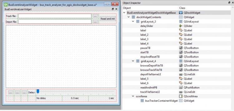
4.12.4 Modifications to the Original Project Files
The next thing we are going to do is make a few smaller changes to the files we copied over from the original project. First of all, it is unfortunately required that we adapt all import statements in which we are importing .py files located in the project folder. The reason is that when we write something like
from core_classes import BusTracker
, this will work fine when the file core_classes.py is located in the current working directory when the program is executed. This is usually the same folder in which the main Python script is located. Therefore, we didn’t have any problems when executing main.py since main.py and the other .py files we wrote are all in the same directory. However, when being run as a QGIS plugin, the working directory will not be the folder containing the plugin code. As a result, you will get error messages when trying to import the other .py files like this. What we have to do is adapt the import statements to start with a dot which tells Python to look for the file in the same folder in which the file in which the import statement appears is located. So the previous example needs to become:
from .core_classes import BusTracker
Here is quick overview of where we have to make these changes:
- In bus_events.py change the import statement at the beginning to:
from .core_classes import Depot, BusTracker
- In bus_track_analyzer.py change the two import statement at the beginning to:
from .bus_events import BusEvent from .core_classes import BusTracker, Observation, Depot
- Lastly, in bus_tracker_widget.py change the import statement at the beginning to:
from .core_classes import BusTracker
In addition to adapting the import statement, we are going to slightly adapt the bus_track_analyzer.py code to better work in concert with the GUI related classes of our plugin code: we are going to add the functionality to emit signals that we can connect to using the QT signal-slot approach. The two signals we are going to add are the following:
- observationProcessed: This signal will be emitted at the end of the nextStep() method, so whenever the BusTrackAnalyzer object is done with processing one observation, the observation object that has just been processed will be included with the signal.
- eventDetected: This signal will be emitted for each new event that is added to the allEvents list. The emitted signal includes the new bus event object.
Both signals will be used to connect an object of a new class we are going to write in Section 4.12.6 that has the purpose of showing the developing bus tracks and detected events live in QGIS. For this, it is required that the object be informed about newly processed observations and newly detected events, and this is what we are going to facilitate with these signals. Luckily, adding these signals to bus_track_analyzer.py just requires you to make a few small changes:
- Add the following PyQt5 import statement somewhere before the line that starts the class definition with “class BusTrackAnalyzer …”:
from PyQt5.QtCore import QObject, pyqtSignal
- To be able to emit signals we need the class BusTrackerAnalyzer to be derived from the QT class QObject we are importing with the newly added import statement. Therefore, please change the first line of the class definition to:
class BusTrackAnalyzer(QObject):
- Then directly before the start of the constructor with “def __init__...", add the following two lines indented relative to the “class BusTrackAnalyzer…” but not part of any method:
observationProcessed = pyqtSignal(Observation) eventDetected = pyqtSignal(BusEvent)
With these two lines we are defining the two signals that can be emitted by this class and the types of the parameters they will include.
- Since we are now deriving BusTrackAnalyzer from QObject, we should call the constructor of the base class QObject from the first line of our __init__(…) method. So please add the following line there:
super(BusTrackAnalyzer, self).__init__()
- The last two changes we need to make are both in the definition of the nextStep() method. We therefore show the entire new version of that method here:
def nextStep(self): """performs next step by processing Observation at the front of the Observations priority queue""" observation = heapq.heappop(self._observationQueue) # get Observation that is at front of queue # go through list of BusEvent subclasses and invoke their detect() method; then collect the events produced # and add them to the allEvents lists for evClass in self._eventClasses: eventsProduced = evClass.detect(observation, self._depotData, self.allBusTrackers) # invoke event detection method self.allEvents.extend(eventsProduced) # add resulting events to event list for event in eventsProduced: self.eventDetected.emit(event) # update BusTracker of Observation that was just processed observation.busTracker.lastProcessedIndex += 1 observation.busTracker.updateSpeed() if observation.busTracker.status == BusTracker.STATUS_STOPPED: # if duration of a stopped event has just expired, change status to "DRIVING" if observation.timepoint.time > observation.busTracker.statusEvent.timepoint.time + observation.busTracker.statusEvent.duration: observation.busTracker.status = BusTracker.STATUS_DRIVING observation.busTracker.statusEvent = None # if this was not the last GPS Timepoint of this bus, create new Observation for the next point and add it to the Observation queue if observation.timepointIndex < len(observation.busTracker.bus.timepoints) - 1: # not last point heapq.heappush(self._observationQueue, Observation(observation.busTracker, observation.timepointIndex + 1) ) # update analyzer status self.lastProcessedTimepoint = observation.timepoint self.observationProcessed.emit(observation)In lines 10 and 11 of this new version we added a for-loop that goes through the events produced by the previous call of detect(…) and emit an eventDetected signal for each using the bus event object as a parameter. In the last line of the method, we do the same with the observationProcessed signal including the just processed Observation object.
4.12.5 Implement Main Functionality in BusTrackAnalyzerForQGISDockWidget class
At this point, our plugin is still missing the code that ties everything together, that is, the code that reads in the data from the input files when the “Read and init” button is clicked and reacts to the control buttons at the bottom of the BusTrackAnalyzerForQGISDockWidget widget by starting to continuously call the analyzer’s nextStep() method, pausing that process, or completely resetting the analysis to start from the beginning. We are going to place the code for this directly in the definition of class BusTrackAnalyzerForQGISDockWidget in bus_track_analyzer_for_qgis_dockwidget.py, so you should open that file for editing now. Here is the code that needs to be added, together with some explanations.
- First, we need to important quite a few classes from our own .py files and also a few additional PyQt5 classes; so please change the import statements at the beginning of the code to the following:
import os from PyQt5 import QtGui, QtWidgets, uic from PyQt5.QtCore import pyqtSignal, QTimer, QCoreApplication # added imports from .bus_track_analyzer import BusTrackAnalyzer from .bus_tracker_widget import BusTrackerWidget #from .qgis_event_and_track_layer_creator import QGISEventAndTrackLayerCreator from .core_classes import Bus, Depot from .bus_events import LeavingDepotEvent, EnteringDepotEvent, BusStoppedEvent, BusEncounterEvent
Note that we again have to use the notation with the dot at the beginning of the module names here. Also, please note that there is one import statement that is still commented out because it is for a class that we have not yet written. That will happen a bit later in Section 4.12.6 and we will then uncomment this line.
-
Next, we are going to add some initialization code to the constructor, directly after the last line of the __init__(…) method saying “self.setupUi(self)”:
# own code added to template file self.running = False # True if currently running analysis self.delay = 0 # delay between steps in milliseconds self.eventClasses = [ LeavingDepotEvent, EnteringDepotEvent, BusStoppedEvent, BusEncounterEvent ] # list of event classes to detect self.busFileColumnIndices = { 'lon': 8, 'lat': 9, 'busId': 5, 'time': 0, 'line': 1 } # dictionary of column indices for required info # create initial BusTrackAnalyzer and BusTrackerWidget objects, and add the later to the scroll area of this widget self.analyzer = BusTrackAnalyzer({}, [], self.eventClasses) self.trackerWidget = BusTrackerWidget(self.analyzer) self.busTrackerContainerWidget.layout().addWidget(self.trackerWidget,0,0) self.layerCreator = None # QGISEventAndTrackLayerCreator object, will only be initialized when input files are read # create a QTimer user to wait some time between steps self.timer = QTimer() self.timer.setSingleShot(True) self.timer.timeout.connect(self.step) # set icons for play control buttons self.startTB.setIcon(QCoreApplication.instance().style().standardIcon(QtWidgets.QStyle.SP_MediaPlay)) self.pauseTB.setIcon(QCoreApplication.instance().style().standardIcon(QtWidgets.QStyle.SP_MediaPause)) self.stopAndResetTB.setIcon(QCoreApplication.instance().style().standardIcon(QtWidgets.QStyle.SP_MediaSkipBackward)) # connect play control buttons and slide to respetive methods defined below self.startTB.clicked.connect(self.start) self.pauseTB.clicked.connect(self.stop) self.stopAndResetTB.clicked.connect(self.reset) self.delaySlider.valueChanged.connect(self.setDelay) # connect edit fields and buttons for selecting input files to respetive methods defined below self.browseTrackFileTB.clicked.connect(self.selectTrackFile) self.browseDepotFileTB.clicked.connect(self.selectDepotFile) self.readAndInitPB.clicked.connect(self.readData)What happens in this piece of code is the following:
- First, we introduce some new instance variables for this class that are needed for reading data and setting up a BusTrackAnalyzer object (you probably recognize the variables eventClasses and busFileColumnIndices from the original main.py file) and for controlling the analysis steps. Variable running will be set to True when the analyzer’s nextStep() method is supposed to be called continuously with small delays between the steps whose length is given by variable delay. It is certainly not optimal that the column indices for the GPS data file are hard-coded here in variable busFileColumnIndices but we decided against including an option for the user to specify these in this version to keep the GUI and code as simple as possible.
- In the next block of code, we create an instance variable to store the BusTrackAnalyzer object we will be using, and we create the BusTrackerWidget widget and place it within the scroll area in the center of the GUI. Since we have not read any input data yet, we are using an empty bus dictionary and empty depot list to set these things up.
- An instance variable for a QTimer object is created that will be used to queue up the execution of the method step() defined later when the widget is in continuous execution mode.
- The next code block simply sets the icons for the different control buttons at the bottom of the widget using standard QT icons.
- Next, we connect the “clicked” signals of the different control buttons to different methods of the class that are supposed to react to these signals. We do the same for the “valueChanged” signal of the QSlider widget in our GUI to be able to adapt the value of the variable delay when the slider is moved by the user.
- Finally, we link the three buttons at the top of the GUI for reading in the data to the respective event handler methods.
-
Now the last thing that needs to happen is adding the different event handler methods we have already been referring to in the previously added code. This is another larger chunk of code since there are quite a few methods to define. Please add the definitions at the end of the file after the definition of the method closeEvent(…) that is already there by default.
# own methods added to template file def selectTrackFile(self): """displays open file dialog to select bus track input file""" fileName, _ = QtWidgets.QFileDialog.getOpenFileName(self,"Select CSV file with bus track data", "","(*.*)") if fileName: self.trackFileNameLE.setText(fileName) def selectDepotFile(self): """displays open file dialog to select depot input file""" fileName, _ = QtWidgets.QFileDialog.getOpenFileName(self,"Select CSV file with depot data", "","(*.*)") if fileName: self.depotFileNameLE.setText(fileName) def readData(self): """reads bus track and depot data from selected files and creates new analyzer and creates analyzer and layer creator for new input""" if self.running: self.stop() try: # read data depotData = Depot.readFromCSV(self.depotFileNameLE.text()) busData = Bus.readFromCSV(self.trackFileNameLE.text(), self.busFileColumnIndices) except Exception as e: QtWidgets.QMessageBox.information(self, 'Operation failed', 'Could not read data from files provided: '+ str(e.__class__) + ': ' + str(e), QtWidgets.QMessageBox.Ok) busData = {} depotData = [] # create new analyzer and layer creator objects and connect them self.analyzer = BusTrackAnalyzer(busData, depotData, self.eventClasses) self.trackerWidget.analyzer = self.analyzer # self.createLayerCreator() self.trackerWidget.updateContent() def stop(self): """halts analysis but analysis can be continued from this point""" self.timer.stop() self.running = False def reset(self): """halts analysis and resets analyzer to start from the beginning""" self.stop() self.analyzer.reset() # self.createLayerCreator() self.trackerWidget.updateContent() def start(self): """starts analysis if analysis isn't already running""" if not self.running: self.running = True self.step() def step(self): """performs a single analysis step of the BusTrackAnalyzer but starts singleshot timer after each step to call itself again""" if self.running: if self.analyzer.isFinished(): self.stop() else: self.analyzer.nextStep() # perform next analysis step self.trackerWidget.updateContent() # redraw tracker widget self.timer.start(max([5,self.delay])) # start timer to call this method again after delay def setDelay(self): """adapt delay when slider has been moved""" self.delay = 10 * self.delaySlider.value() if self.running: # if analysis is running, change to the new delay immediately self.timer.stop() self.timer.start(max([5,self.delay]))
The first two methods selectTrackFile() and selectDepotFile() are called when the “…” buttons at the top are clicked and will open file dialog boxes for picking the input files. The method readData() is invoked when the “Read and init” button is clicked. It stops all ongoing executions of the analyzer, attempts to read the data from the selected files, and then creates a new BusTrackAnalyzer object for this input data and connects it to the BusTrackerWidget in our GUI. The code of this function contains another two lines that are commented out and that we will uncomment later.
The other methods we define in this piece of code are the event handler functions for the control buttons at the bottom:
- stop() is called when the “Pause” button in the middle is clicked and simply stops the timer if its currently running and sets the variable running to False so that the analyzer’s nextStep() method won’t be called anymore.
- reset() is called when the control button on the left is called and it also stops the execution but, in addition, resets the analyzer so that the analysis will start from the beginning when the “Start” button is clicked again.
- start() is called when the right control button (“Play”) for continuously performing analysis steps is clicked. It sets variable running to True and then invokes method step() to run the first analysis step.
- step() is either called from start() or by the timer it sets up itself after each call of the analyzer’s nextStep() method to perform the next analysis step after a certain delay until all observations have been processed. Please note that we are using minimum delay of 5 milliseconds to make sure that the QGIS GUI remains responsive while we are running the analysis.
- setDelay() is called when the slider is moved and it translates the slider position into a delay value between 0 and 1 second. It also immediately restarts the timer to use this new delay value.
Our plugin is operational now and you can open QGIS and run it. In case you already have QGIS running or you encounter any errors that need to be fixed, don’t forget to reload the plugin code with the help of the Plugin Reloader plugin. Once the dock widget appears at the right side of the QGIS window (as shown in the figure below), do the following:
- Use the “…” buttons to select the input files for the bus GPS and depot data.
- Click “Read and init”; after that you should see the initial bus tracker configuration in the central area of the dock widget.
- Press the “Play” button to start the analysis; the content of the BusTrackerWidget should now continuously update to reflect the current state of the analysis
- Test out the “Pause” and “Rewind” buttons as well as changing the delay between steps with the slider to control the speed the analysis is run at.
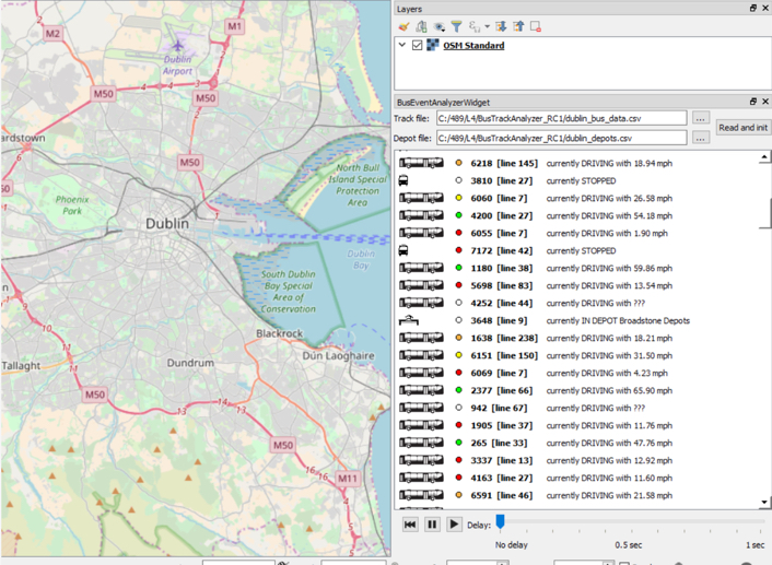
So far, so good. We have now turned our original standalone project into a QGIS plugin and even added in some extra functionality allowing the user to pause and restart the analysis and control the speed. However, typically a QGIS plugin in some way interacts with the content of the project that is currently open in QGIS, for instance by taking some of its layers as input or adding new layers to the project. We will add this kind of functionality in the next section and this will be the final addition we are making to our plugin.
4.12.6 Create and Integrate New Class QGISEventAndTrackLayerCreator
In addition to showing the current bus tracker states in the dock widget, we want our plugin to add two new layers to the currently open QGIS project that show the progress of the analysis and, once the analysis is finished, contain its results. The two layers will correspond to the two output files we produced in the original project in Section 4.10:
- a polyline layer showing routes taken by the different bus vehicles with the bus IDs as attribute,
- a point layer showing the detected events with the type of the event and a short description as attributes.
Since we don’t want to just produce these layers at the end of the analysis but want these to be there from the start of the analysis and continuously update whenever a new bus GPS observation is processed or an event is detected, we are going to write some code that reacts to the observationProcessed and eventDetected signals emitted by our class BusTrackAnalyzer (see the part of Section 4.12.4 where we added these signals). We will define a new class for all this that will be called QGISEventAndTrackLayerCreator and it will be defined in a new file qgis_event_and_track_layer_creator.py. The class definition consists of the constructor and two methods called addObservationToTrack(…) and addEvent(…) that will be connected to the corresponding signals of the analyzer.
Let’s start with the beginning of the class definition and the constructor. All following code needs to be placed in file qgis_event_and_track_layer_creator.py that you need to create in the plugin folder.
import qgis
class QGISEventAndTrackLayerCreator():
def __init__(self):
self._features = {} # dictionary mapping bus id string to polyline feature in bus track layer
self._pointLists = {} # dictionary mapping bus id string to list of QgsPointXY objects for creating the poylines from
# get project currently open in QGIS
currentProject = qgis.core.QgsProject.instance()
# create track layer and symbology, then add to current project
self.trackLayer = qgis.core.QgsVectorLayer('LineString?crs=EPSG:4326&field=BUS_ID:integer', 'Bus tracks' , 'memory')
self.trackProv = self.trackLayer.dataProvider()
lineMeta = qgis.core.QgsApplication.symbolLayerRegistry().symbolLayerMetadata("SimpleLine")
lineLayer = lineMeta.createSymbolLayer({'color': '0,0,0'})
markerMeta = qgis.core.QgsApplication.symbolLayerRegistry().symbolLayerMetadata("MarkerLine")
markerLayer = markerMeta.createSymbolLayer({'width': '0.26', 'color': '0,0,0', 'placement': 'lastvertex'})
symbol = qgis.core.QgsSymbol.defaultSymbol(self.trackLayer.geometryType())
symbol.deleteSymbolLayer(0)
symbol.appendSymbolLayer(lineLayer)
symbol.appendSymbolLayer(markerLayer)
trackRenderer = qgis.core.QgsSingleSymbolRenderer(symbol)
self.trackLayer.setRenderer(trackRenderer)
currentProject.addMapLayer(self.trackLayer)
# create event layer and symbology, then add to current project
self.eventLayer = qgis.core.QgsVectorLayer('Point?crs=EPSG:4326&field=TYPE:string(50)&field=INFO:string(255)', 'Bus events' , 'memory')
self.eventProv = self.eventLayer.dataProvider()
colors = { "BusEncounterEvent": 'yellow', "BusStoppedEvent": 'orange', "EnteringDepotEvent": 'blue', "LeavingDepotEvent": 'green' }
categories = []
for ev in colors:
categories.append( qgis.core.QgsRendererCategory( ev, qgis.core.QgsMarkerSymbol.createSimple({'name': 'square', 'size': '3.0', 'color': colors[ev]}), ev ))
eventRenderer = qgis.core.QgsCategorizedSymbolRenderer("TYPE", categories)
self.eventLayer.setRenderer(eventRenderer)
currentProject.addMapLayer(self.eventLayer)
To be able to build polylines for the bus tracks and update these whenever a new observation has been processed by the analyzer, we need to maintain dictionaries with the QGIS features and point lists for each bus vehicle track. These are created at the beginning of the constructor code in lines 6 and 7. In addition, the constructor accesses the currently open QGIS project (line 10) and adds the two new layers called “Bus tracks” and “Bus events” to it (lines 29 and 44). The rest of the code is mainly for setting the symbology of these two layers: For the track layer, we use black lines with a red circle marker at the end to indicate the current location of the vehicle (lines 16 to 27) as shown in the image below. For the events, we use square markers in different colors based on the TYPE of the event (lines 35 to 42).
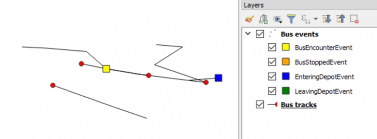
Now we are going to add the definition of the method addObservationToTrack(…) that will be connected to the observationProcessed signal emitted when the analyzer object has completed the execution of nextStep().
def addObservationToTrack(self, observation):
"""add new vertex to a bus polyline based on the given Observation object"""
busId = observation.busTracker.bus.busId;
# create new point for this observation
p = qgis.core.QgsPointXY(observation.timepoint.lon, observation.timepoint.lat)
# add point to point list and (re)create polyline geometry
if busId in self._features: # we already have a point list and polyline feature for this bus
feat = self._features[busId]
points = self._pointLists[busId]
points.append(p)
# recreate polyline geometry and replace in layer
polyline = qgis.core.QgsGeometry.fromPolylineXY(points)
self.trackProv.changeGeometryValues({feat.id(): polyline})
else: # new bus id we haven't seen before
# create new polyline and feature
polyline = qgis.core.QgsGeometry.fromPolylineXY([p])
feat = qgis.core.QgsFeature()
feat.setGeometry(polyline)
feat.setAttributes([int(busId)])
_, f = self.trackProv.addFeatures([feat])
# store point list and polyline feature in respective dictionaries
self._features[busId] = f[0]
self._pointLists[busId] = [p]
# force redraw of layer
self.trackLayer.triggerRepaint()
qgis.utils.iface.mapCanvas().refresh()
The Observation object given to this method as a parameter provides us with access to all the relevant information we need to update the polyline feature for the bus this observation is about. First, we extract the ID of the bus (line 3) and create a new QgsPointXY object from the Timepoint stored in the Observation object (line 6). If we already have a polyline feature for this vehicle, we get the corresponding feature and point lists from the features and pointLists dictionaries, add the new point to the point list and create a new polyline geometry from it, and finally change the geometry of that feature in the bus track layer to this new geometry (lines 10 to 16). If instead this is the first observation of this vehicle, we create a point list for it to be stored in the pointList dictionary as well as a new polyline geometry with just that single point, and we then set up a new QgsFeature object for this polyline that is added to the bus track layer and also the features dictionary (lines 19 to 27). At the very end of the method, we make sure that the layer is repainted in the QGIS map canvas.
Now we add the code for the addEvent(…) method completing the definition of our class QGISEventAndTrackLayerCreator:
def addEvent(self, busEvent):
"""add new event point feature to event layer based on the given BusEvent object"""
# create point feature with information from busEvent
p = qgis.core.QgsPointXY(busEvent.timepoint.lon, busEvent.timepoint.lat)
feat = qgis.core.QgsFeature()
feat.setGeometry(qgis.core.QgsGeometry.fromPointXY(p))
feat.setAttributes([type(busEvent).__name__, busEvent.description()])
# add feature to event layer and force redraw
self.eventProv.addFeatures([feat])
self.eventLayer.triggerRepaint()
qgis.utils.iface.mapCanvas().refresh()
This method is much simpler because we don’t have to modify existing features in the layer but rather always add one new point feature to the event layer. All information required for this is taken from the bus event object given as a parameter: The coordinates for the next point feature are taken from the Timepoint stored in the event object (line 4), for the TYPE field of the event we take the type of the event object (line 7), and for the INFO field we take the string returned by calling the event object’s description(…) method (also line 7).
To incorporate this new class into our current plugin, we need to make a few more modifications to the class BusTrackAnalyzerForQGISDockWidget in file bus_track_analyzer_for_qgis_dock_widget.py. Here are the instructions for this:
- Remove the # at the beginning of the line “from .qgis_event_and_track_layer_creator import …” to uncomment this line and import our new class.
- Now we add a new auxiliary method to the class definition that has the purpose of creating an object of our new class BusTrackAnalyzerForQGISDockWidget and connecting its methods to the corresponding signals of the analyzer object. Add the following definition as the first method after the “closeEvent” method, so directly after the comment “# own methods added to the template file”.
def createLayerCreator(self): """creates a new QGISEventAndTrackLayerCreator for showing events and tracks on main QGIS window and connects it to analyzer""" self.layerCreator = QGISEventAndTrackLayerCreator() self.analyzer.observationProcessed.connect(self.layerCreator.addObservationToTrack) self.analyzer.eventDetected.connect(self.layerCreator.addEvent)We already set up an instance variable layerCreator in the constructor code and we are using it here for storing the newly created layer creator object. Then we connect the signals to the two methods of the layer creator object.
- Now we just need to uncomment two lines to make sure that the method createLayerCreator() is called at the right places, namely after we read in data from the input files and when the analyzer is reset. In both cases, we want to create a new layer creator object that will set up two new layers in the current QGIS project. The lines that you need to uncomment for this by removing the leading # are:
- the line “# self.createLayerCreator()” in method readData()
- the line “# self.createLayerCreator()” in method reset()
You should make sure that the indentation is correct after removing the hashmarks.
That’s it, we are done with the code for our plugin!
4.12.7 Try It Out
To try out this new version of the plugin, close the dock widget if it’s currently still open in QGIS and then run the Plugin Reloader plugin to load this updated version of our plugin. Add a basemap to your map project and zoom it to the general area of Dublin. When you then load the input files, you will see the two new layers appear in the layer list of the current QGIS project with the symbology we are setting up in the code. When you now start the analysis, what you see should look like the video below with the bus tracker widget continuously updating the bus status information, the bus tracks starting to appear in the QGIS map window, and square symbols starting to pop up for the events detected.
[NOTE: This video (3:04) does NOT contain sound]
The delay slider can be used to increase the breaks between two analysis steps, which can be helpful if the map window doesn’t seem to update properly because QGIS has problems catching up with the requests to repaint layers. This in particular is a good idea if you want to pan and zoom the map in which case you may notice the basemap tiles not appearing if the delay is too short.
Overall, there is quite a bit that could be optimized to make sure that QGIS remains responsive while the plugin and analysis are running as well as other improvements and extensions that could be made. But all this would increase the amount of code needed quite a bit and this has already been a rather long project to begin with, requiring you to read and understand a lot of code. As we said before, it is not required to understand each line in the code; the crucial points to understand are how we are using classes, objects, and inheritance in this project and make use of the other techniques and concepts taught in this lesson. Reading and understanding other people’s code is one of the main ways to become a better programmer and since we are approaching the end of this course, this was a good place to practice this a bit and maybe provide some inspiration for your term project. However, we certainly don’t expect your term project to be nearly as complex as the plugin created in this section!
4.13 Lesson 4 Practice Exercise
The focus in this lesson has been on object-oriented programming in Python and applying it in the context of QGIS to create GUI-based programs and plugins. In the only practice exercise of this lesson, we are going to apply the concepts of self-defined classes, inheritance and overriding methods to build a standalone GIS tool based on the qgis package that is significantly simpler than the project from the lesson walkthroughs. As before, this is intended as a preparation for this lesson's homework assignment in which you are supposed to create a somewhat larger object-oriented tool.
Here is the task: You have been given a .csv file that contains observations of animals in Kruger National Park. Each row in the .csv file contains a unique ID for the observed animal and the latitude and longitude coordinates of the observation, in that order. The observations are ordered chronologically. The test file we will be working with has just the following nine rows. Please download the L4exercise_data.zip file containing this data.
123AD127,-23.965517,31.629621 183AE121,-23.921094,31.688953 223FF097,-23.876783,31.661707 183AE121,-23.876783,31.661707 123AD121,-23.961818,31.694983 223FF097,-24.083749,31.824532 123AD127,-24.083749,31.824532 873TF129,-24.040581,31.426711 123AD127,-24.006232,31.428593
The goal is to write a standalone qgis script that produces a point GeoPackage file with a point feature for just the first observation of each animal occurring in the .csv file. The file contains observations for five different animals and the result when opened in QGIS should look like this:
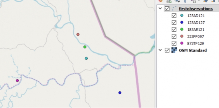
You have already produced some code that reads the data from the file into a pandas data frame stored in variable data. You also want to reuse a class PointObject that you already have for representing point objects with lat and lon coordinates and that has a method called toQgsFeature(…) that is able to produce and return a QgsFeature (see again Section 4.5.3) for a point object of this class.
import qgis
import sys, os
import pandas as pd
# create pandas data frame from input data
data = pd.read_csv(r"C:\489\L4\exercise\L4exercise_data.csv")
class PointObject():
# constructor for creating PointObject instances with lon/lat instance variables
def __init__(self, lat, lon):
self.lon = lon
self.lat = lat
# methods for creating QgsFeature object from a PointObject instance
def toQgsFeature(self):
feat = qgis.core.QgsFeature()
feat.setGeometry(qgis.core.QgsGeometry.fromPointXY(qgis.core.QgsPointXY(self.lon, self.lat)))
return feat
firstObservations = [] # for storing objects of class pointWithID
firstObservationsFeatures = [] # for storing objects of class QgsFeature
When you look at method toQgsFeature(), you will see that it creates a new QgsFeature (see Section 4.5.3), sets the geometry of the feature to a point with the given longitude and latitude coordinates, and then returns the feature. Since PointObject does not have any further attributes, no attributes are defined for the created QgsFeature object.
Your plan now is to write a new class called PointWithID that is derived from the class PointObject and that also stores the unique animal ID in an instance variable. You also want to override the definition of toQgsFeature() in this derived class (see again Section 4.7), so that it also uses setAttributes(…) to make the ID of the animal an attribute of the produced QgsFeature object. To do this, you can first call the toQgsFeature() method of the base class PointObject with the command
super(PointWithID, self).toQgsFeature()
… and then take the QgsFeature object returned from this call and set the ID attribute for it with setAttributes(…).
Furthermore, you want to override the == operator for PointWithID so that two objects of that class are considered equal if their ID instance variable are the same. This will allow you to store the PointWithID objects created in a list firstObservations and check whether or not the list already contains an observation for the animal in a given PointWithID object in variable pointWithID with the expression
pointWithID in firstObservations
To override the == operator, class PointWithID needs to be given its own definition of the __eq__() method as shown in Section 4.6.2.
What you need to do in this exercise is:
- Define the class PointWithID according to the specification above.
- Add the code needed for making this a standalone qgis program (Sections 4.5.4 and 4.10.2.4).
- Implement a loop that goes through the rows of the pandas data frame (with data.itertuples(), Section 3.8.2) and creates an object of the class PointWithID for the given row, then adds this object to list firstObervations, unless the list already contains an object with the same animal ID.
- Add the code for creating the new point layer with EPSG:4326 as the CRS.
- Make firstObservationFeatures a list with a QgsFeature object for each PointWithID object in list firstObservations using the overridden toQgsFeature() method. Then add all features from that new list to the new layer (Section 4.5.3).
- Finally, write the new layer to a new GeoPackage file and check whether or not you get the same result as shown in the image above.
4.13.1 Lesson 4 Practice Exercise Solution and Explanation
Solution
import qgis
import qgis.core
import sys, os
import pandas as pd
# read data into pandas data frame
data = pd.read_csv(r"C:\489\L4\exercise\L4exercise_data.csv")
# class definition for PointObject
class PointObject():
def __init__(self, lat, lon):
self.lon = lon
self.lat = lat
def toQgsFeature(self):
feat = qgis.core.QgsFeature()
feat.setGeometry(qgis.core.QgsGeometry.fromPointXY(qgis.core.QgsPointXY(self.lon, self.lat)))
return feat
firstObservations = [] # for storing objects of class pointWithID
firstObservationsFeatures = [] # for storing objects of class QgsFeature
# code for creating QgsApplication and initializing QGIS environment
qgis_prefix = os.getenv("QGIS_PREFIX_PATH")
qgis.core.QgsApplication.setPrefixPath(qgis_prefix, True)
qgs = qgis.core.QgsApplication([], False)
qgs.initQgis()
# definition of class PointWithID derived from PointObject
# to represent animal observation from the input data
class PointWithID(PointObject):
def __init__(self, pID, lat, lon):
super(PointWithID, self).__init__(lat, lon)
self.pID = pID # instance variable for storing animal ID
# overwriting the == operator to be based on the animal ID
def __eq__(self, other):
return self.pID == other.pID
# overwriting this method to include animal ID as attribute of QgsFeature created
def toQgsFeature(self):
feat = super(PointWithID, self).toQgsFeature()
feat.setAttributes([self.pID])
return feat
# create list of PointWithID object with first observations for each animal in the data frame
for row in data.itertuples(index=False):
pointWithID = PointWithID(row[0], row[1], row[2])
if not pointWithID in firstObservations: # here __eq__() is used to do the comparison
firstObservations.append(pointWithID)
# list comprehension for creating list of features from firstObservations list
firstObservationsFeatures = [ o.toQgsFeature() for o in firstObservations ]
# create new point layer with field for animal ID
layer = qgis.core.QgsVectorLayer("Point?crs=EPSG:4326&field=AnimalID:string(255)", 'animal first observations' ,'memory')
# add features to new layer
prov = layer.dataProvider()
prov.addFeatures(firstObservationsFeatures)
# save layer as GeoPackage file
qgis.core.QgsVectorFileWriter.writeAsVectorFormat( layer, r"C:\489\L4\exercise\firstobservations.gpkg", "utf-8",layer.crs(), "GPKG")
# clean up
qgs.exitQgis()
Explanation
- In line 34 the new class PointWithID is declared to be derived from class PointObject.
- The constructor in line 36 calls the constructor of the base class and then adds the additional instance variable for the animal ID (called pID).
- __eq__() is defined in lines 43 and 44 to compare the pID instance variables of both involved objects and return True if they are equal.
- In lines 48 and 49, we call toQgsFeature() of the base class PointObject and then take the returned feature and add the animal ID as the only attribute.
- In lines 53 to 56, we use itertuples() of the data frame to loop through its rows. We create a new PointWithID object in variable pointWithID from the cell values of the row and then test whether an object with that ID is already contained in list firstObservations. If not, we add this object to the list.
- In line 59, we use toQgsFeature() to create a QgsFeature object from each PointWithID object in the list. These are then added to the new layer in line 66.
- When creating the new layer in line 62, we have to make sure to include the field for storing the animal ID in the string for the first parameter.
4.14 Lesson 4 Assignment
In this final homework assignment, the task is to create a qgis based program, simpler than the Bus Track Analyzer from the lesson walkthrough but also involving the definition of a class hierarchy and static class functions to identify instances of the classes in the input data. While it is an option to submit a QGIS plugin rather than a standalone tool for over&above points, this is not a requirement and, therefore, it is not needed that you have worked through Section 4.11 and 4.12 in detail. The main code for the tool you are going to implement will include a class hierarchy with classes for different types of waterbodies (streams, rivers, lakes, ponds, etc.) and the tool's purpose will be to create two new vector data sets from a JSON data export from OpenStreetMap (OSM).
The situation is the following: you are working on a hydrology related project. As part of the project you frequently need detailed and up-to-date vector data of the waterbodies in different areas and one source you have been using to obtain this data is OpenStreetMap. To get the data you are using the Overpass API running queries like the following
https://www.overpass-api.de/api/interpreter?data=[out:json];(way["natural"="water"](40.038844,-79.006452,41.497860,-76.291359);way["waterway"] (40.038844,-79.006452,41.497860,-76.291359););(._;>;);out%20body;
to obtain all OSM “way” elements (more on ways and the OSM data model in a moment) with certain water related tags.
An overpass query like this will return a JSON document listing all the way entities with the required tags and their nodes with coordinates. Nodes are point features with lat / lon coordinates and ways are polyline or polygon features whose geometry is defined via lists of nodes. If you are not familiar with the OSM concepts of nodes, ways, and relations, please take a moment to read “The OpenStreetMap data model."
The only data you will need for this project is the JSON input file we will be using. Download it and extract it to a new folder, then open it in a text editor. You will see that the JSON code in the file starts with some meta information about the file and then has an attribute called “elements” that contains a list of all OSM node elements followed by all OSM way elements (you have to scroll down to the end to see the way elements because there are many more nodes than ways in the query result).
All node definitions in the “elements” list have the following structure:
{
"type": "node",
"id": 25446505,
"lat": 40.2585099,
"lon": -77.0521733
},
The “type” attribute makes it clear that this JSON element describes an OSM node. The “id” attribute is a unique identifier for the node and the other two attributes are the latitude and longitude coordinates.
All way definitions in the “elements” list have the following structure:
{
"type": "way",
"id": 550714146,
"nodes": [
5318993708,
5318993707,
5318993706,
...
5318993708
],
"tags": {
"name": "Wilmore Lake",
"natural": "water",
"water": "reservoir"
}
},
The attribute “type” signals that this JSON element describes an OSM way feature. The “id” attribute contains a unique ID for this way and the “nodes” attribute contains a list of node IDs. If the IDs of the first and last nodes in this list are identical (like in this case), this means that this is a closed way describing an areal polygon geometry, rather than a linear polyline geometry. To later create QGIS geometries for the different waterbodies, you will have to take the node list of a way, look up the corresponding nodes based on their IDs, and take their coordinates to create the polygon or polyline feature from.
In addition, the JSON elements for ways typically (but not always!) contain a “tags” attribute that stores the OSM tags for this way. Often (but not always!), ways will have a “name” tag (like in this case) that you will have to use to get the name of the feature. In this example, the way also has the two tags “natural” with the value “water” assigned and “water” with the value “pond” assigned. The way in which waterbodies are tagged in OSM has been criticized occasionally and suggestions for improvements have been made. Right now, waterbodies typically either have been tagged with the key “waterway” with the assigned value being a particular type like “stream” or “river”, or with the combination of the key “natural” being assigned the value “water” and the key “water” being assigned a specialized type like “lake” or “pond”. Luckily, you don’t have to worry too much about the inconsistencies and disadvantages of the OSM tagging for waterbodies because you will below be given concrete rules on how to identify the different types of waterbodies we are interested in.
In lesson 2, we already talked about JSON code and that it can be turned into a nested Python data structure that consists of lists and dictionaries. In lesson 2, we got the JSON from web requests and we therefore used the requests module for working with the JSON code. In the context of this assignment, it makes more sense to use the json module from the standard library to work with the provided JSON file. You can simply load the JSON file and create a Python data structure from the content using the following code assuming that the name and path to the input file are stored in variable filename:
import json with open(filename, encoding = "utf8") as file: data = json.load(file)
After this, you can, for instance, use the expression data["elements"] to get a list with the content that is stored in the top-level “elements” attribute. To get the first element from that list which will be the description of an OSM node, you'd use data["elements"][0] and data["elements"][0]["id"] refers to the ID of that node, while data["elements"][0]["type"]will return the string 'node' providing a way to check what kind of OSM element you are dealing with. The page “How-to-parse-json-string-in-python” contains an example of how to access elements at different levels in the JSON structure that might be helpful here. If you have any questions about handling JSON code while working on this assignment, please ask them on the forums.
In order to later create polyline or polygon geometries from the OSM way elements in the input file, we will have to look up node elements based on the node IDs that we find in the "nodes" lists of the way elements to get to the latitude and longitude coordinates of these nodes. A good first step, therefore, is to create seperate dictionaries for the node and way elements using the IDs as key such that we can use the IDs to get to the entire node or way description as a Python dictionary. The following code creates these dictionaries from the content of variable data:
nodesDict = {} # create empty dictionary for the node elements
waysDict = {} # create empty dictionary for the way elements
for element in data['elements']: # go through all elements in input data
if element['type'] == 'node': # check if element is an OSM node
nodesDict[element['id']] = element # place element in nodes dictionary using its ID as the key
elif element['type'] == 'way': # check if element is an OSM way
waysDict[element['id']] = element # place element in ways dictionary using its ID as the key
Now that this is done we can loop through all way elements using the following code:
for wayID in waysDict: # go through all keys (= way IDs) way = waysDict[wayID] # get the way element for the given ID print(way) ... # do something else with way, e.g. access its node list with way['nodes']
Since each node or way element is again represented by a Python dictionary, the output we get from the print statement will look as below and we can, for instance, use way['nodes'] or way['tags'] to refer to the different properties of the way element.
{'type': 'way', 'id': 4251261, 'nodes': [25446505, 618262874, 25446506, 618262877, 618262880, 5421855904, 25446508, 4568980789, 4568980790, 4568980791, 4568980792, 618264570, 4568980793, 4568980794, 4568980795, 618264571, 25446510, 4568980796, 4568980797, 618264572, 4568980798, 4568980799, 618264573, 4568980800, 25446511, 618264574, 25446512, 618264575, 25446513, 618264576, 618264577, 25446514, 618264578, 25446516, 5417811540, 618264580, 25446560, 25446517], 'tags': {'name': 'Conodoguinet Creek', 'waterway': 'river'}}
Furthermore, whenever we have a node ID and need to get the information for that node, we can look it up in the nodes dictionary:
nodeID = 5318993708 # some exemplary node ID node = nodesDict[nodeID] # get the node element we have stored under that ID print(node)
Again, keep in mind that a node is represented by a Python dictionary. Hence, the output from the print statement will look as below and we can, for instance, use node['lat'] and node['lon'] to refer to the latitude and longitude coordinates of that node.
{'type': 'node', 'id': 5318993708, 'lat': 40.4087294, 'lon': -78.6877245}
Before you read on, we recommend that you make sure you have a good understanding of what the code above does and how to work with the nested dictionary structures containing the way and node information. Play around with the code a bit. For instance, try to modify the loop that goes through the way elements such that it checks whether or not the given way elements contain a 'tags' property and if so, whether or not the tags dictionary contains an 'name' entry. If so, print out the name stored there. E.g. for the first way element shown above, the produced output should be just Conodoguinet Creek.
Your task
Your task now is to implement a tool based on the qgis Python package with at least a basic GUI that allows the user to select an input .json file on disk. When the user presses a button, the tool reads in all the node and way information from the json file into two dictionaries that allow for accessing the different node and way entities by their ID as we showed above.
Next, the program should loop through all the way entities and create objects of the six different waterbody classes Stream, River, Canal, Lake, Pond, and Reservoir depending on how the ways are tagged. The first three of these classes are for linear features that will be represented by polylines later on. The other three are for areal features that will be represented by polygons. Your tool should produce two new vector data sets in the GeoPackage format, one with all linear features and one with all areal features that look as shown in the image below when added to QGIS.
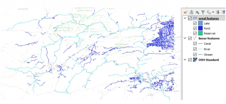
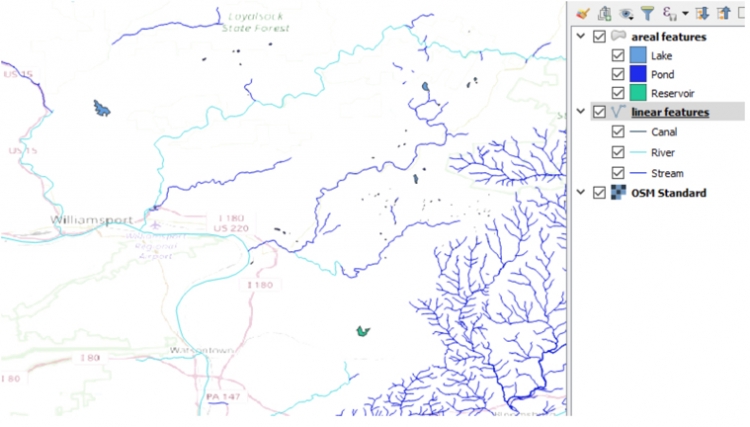
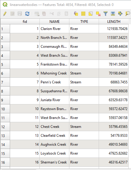
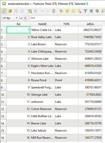
Details
Waterbody class hierarchy:
The classes for the different waterbody types should be arranged in a class hierarchy that looks as in the image below (similar to the bus event hierarchy from the lesson walkthroughs, see also Section 4.7 again). In the end, there should be definitions for all these 9 classes and the different instance variables, methods, and static class functions should be defined at the most suitable locations within the hierarchy. A template file for this class hierarchy that already contains (partial) definitions of some of the classes will be provided below as a starting point.
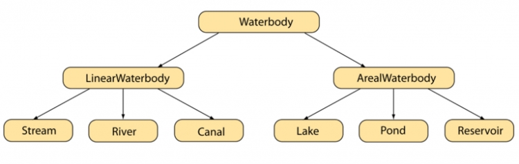
Here are a few requirements for the class hierarchy:
- The entire class hierarchy should be defined in its own file, similar to the bus_events.py file in the lesson walkthroughs.
- Each waterbody object should have an instance variable called name for storing the name of this waterbody, e.g., 'Wilmore Lake'. If there is no “name” tag in the JSON code, the name should be set to “unknown”.
- Each waterbody object should have an instance variable called geometry for storing the geometry of the waterbody as a qgis QgsGeometry object. You will have to create this geometry from the node lists of a way using either the fromPolylineXY(…) or fromPolygonXY(…) functions defined in the QgsGeometry class depending on whether we are dealing with a linear or areal waterbody (see examples from the lesson content, e.g. Section 4.10.2.4). Both functions take QgsPointXY objects as input but in the case of fromPolylineXY(…) it's a single list of QgsPointXY objects, while for fromPolygonXY(...) it's a list of lists of QgsPointXY objects because the polygons can in principle contain polygonal holes.
- Each object of a linear waterbody class should have an instance variable called length for storing its length in meters, while each object of an areal waterbody class should have an instance variable called area for storing its area in square meters. The values for these instance variables can be computed using the approach shown under “Hint 2” below once the geometry object has been created from the nodes. This is already implemented in template class hierarchy file provided below.
- There should be a static class function (see Section 4.8) fromOSMWay(way, allNodes) for all waterbody classes that takes the Python data structure for a single OSM way element and the dictionary containing all OSM node elements read from the input file as parameters. The function then checks the tags of the given way element to see whether or not this element describes a waterbody of the given class and if so creates and returns a corresponding object of that class. For example: If fromOSMWay(way, allNodes) is called for class Stream, the implementation of this function in class Stream needs to check whether or not the tags match the rules for the Stream class (see tag rule list given below). If yes, it will then create a polyline geometry from the node ID list included in the way element by looking up the coordinates for each node in the allNodes dictionary. Then it will create an object of class Stream with the created geometry and, if available, name extracted from the “name” tag of the way. If the tags do not match the rule for Stream, the function simply returns None, signaling that no object was created. Overall this function should work and be used similarly to the detect(…) class functions of the bus event classes from the lesson walkthroughs. The following code provides a basic example of how the function could be used and tested:
import waterbodies # import the file with the waterbodies class hierarchy classes = [ waterbodies.Stream ] # list of bottom level classes from the waterbodies.py file; we just use the Stream class in this example but the list can later be extended way1 = waysDict[5004497] # we just work with two particular way elements from our waysDict dictionary in this example; this one is actually a stream ... way2 = waysDict[4251261] # ... while this one is not a stream for cl in classes: # go through the classes in the class list print('way1:') result = cl.fromOSMWay(way1, nodesDict) # call the fromOSMWay(...) static class function of the given class providing a way element and our nodes dictionary as parameters; # the task of the function is to check whether the way element in the first parameter satisfies the tag rules for the class (e.g. for Stream) and, # if yes, create a new object of that class (e.g. an object of class Stream) and return it. To create the object, the function has to create a QgsGeometry # object from the list of node IDs listed in the way element first which involves looking up the coordinates of the nodes in the nodes dictionary provided # in the second parameter if result: # test whether the result is not None meaning that the tag rules for the class were satisfied and an object has been created and returned print('object created: ' + str(result)) # since way1 is indeed a Stream this will print out some information about the created object else: print('return value is None -> no object of class ' + str(cl) + ' has been created') print('way2:') result = cl.fromOSMWay(way2, nodesDict) # now we do the same for way2 which is NOT a stream if result: # test whether the result is not None meaning that the tag rules for the class were satisfied and an object has been created and returned print('object created: ' + str(result)) else: print('return value is None -> no object of class ' + str(cl) + ' has been created') # since way2 is not a stream, this line will be executedOf course, you will only be able to test run this piece of code once you have implemented the fromOSMWay(...) static class function for the Stream class in the waterbodies class hiearchy file. But here is what the output will look like:way1: object created: <waterbodies.Stream object at 0x000000F198A2C4E0> way2: return value is None -> no object of class <class 'waterbodies.Stream'> has been created
Also, the idea of course is that later fromOSMWay(...) will be called for all way elements in the waysDict dictionary, not for particular elements like we are doing in this example. - There should be a method toQgsFeature(self) that can be invoked for all waterbody objects. This method is supposd to create and return a QgsFeature object for the waterbody object it is invoked on. The returned QgsFeature object can then be added to one of the output GeoPackage files. When called for an object of a linear waterbody class, the created feature should have the polyline geometry of that object and at least the attributes NAME, TYPE, and LENGTH as shown in the image of the linear attribute table above. When called for an areal waterbody class, the created feature should have the polygon geometry of that object and at least the attributes NAME, TYPE, and AREA (see the image with the areal attribute table above). Using this method to create a QgsGeometry object can be integrated into the for-loop of the example code from the previous point:
if result: # test whether the result is not None meaning the tag rules for class where satisfied an object has been created and returned feature = result.toQgsFeature() # call toQgsFeature() to create a QgsFeature object from the waterbody object print(feature) # print string representation of feature print(feature.attributes()) # print attribute values as a list # do something else with feature like storing it somewhere for later use
Assuming this code is executed for way1, running the code after the toQgsFeature() method has been implement should produce the following output:<qgis._core.QgsFeature object at 0x000000AB6E36F8B8> ['Rapid Run', 'Stream', 372.01922201444535]
The attributes listed are the name, the type, and the length of the stream. - Add a definition of the __str__(self) method to each class at the bottom level of the hierarchy with the goal of producing a nicer description of the object than simply something like <waterbodies.Stream object at 0x000000F198A2C4E0>. The description should include the type, name, and length/area of the object, so for example it could look like this:
Stream Rapid Run (length: 372.01922201444535m)
While this method will not play an important role in the final version of the code for this assignment, it can be very useful to provide some helpful output for debugging. Keep in mind that, once you have defined this method, using print(result) or str(result) in the code examples for fromOSMWay(...) will produce this more readable and more informative description instead of just <waterbodies.Stream object at 0x000000F198A2C4E0>.
Tag rules for different waterbodies
We already mentioned that we are providing the tag rules for the six bottom-level classes in the hierarchy that should be used for checking whether or not a given OSM way describes an instance of that class. You simply will have to turn these into Python code in the different versions of the fromOSMWay(way, allNodes) static class function in your class hierarchy. Here are the rules:
Stream: the way has the “tags” attribute and among the tags is the key “waterway” with the value “stream” assigned.
River: the way has the “tags” attribute and among the tags is the key “waterway” with the value “river” assigned.
Canal: the way has the “tags” attribute and among the tags is the key “waterway” with the value “canal” assigned.
Lake: the way has the “tags” attribute and among the tags there is both, the key “natural” with the value “water” assigned and the key “water” with the value “lake” assigned.
Pond: the way has the “tags” attribute and among the tags there is both, the key “natural” with the value “water” assigned and the key “water” with the value “pond” assigned.
Reservoir: the way has the “tags” attribute and among the tags there is both, the key “natural” with the value “water” assigned and the key “water” with the value “reservoir” assigned.
Right now, the rules for all three linear classes are the same except for the specific value that needs to be assigned to the “waterway” key. Similarly, the rules for all three areal classes are the same except for the specific value that needs to be assigned to the “water” key. However, since these rules may change, the logic for checking the respective conditions should be implemented in the fromOSMWay(way, allNodes) class function for each of these six classes.
Creation of output GeoPackage files:
You saw examples of how to create new layers and write them to GeoPackage files with qgis in Section 4.5.3 and the lesson walkthrough code from Section 4.10 (main.py and bus_track_analyzer.py). So once you have gone through the list of way elements in the input data and created waterbody objects of the different classes via the fromOSMWay(...) static class functions, creating the features by calling the toQgsFeature() method of each waterbody object and producing the output files should be relatively easy and just require a couple lines of code. You will have to make sure to use the right geometry type and CRS when creating the layers with qgis.core.QgsVectorLayer(...) though.
GUI:
As in the Lesson 2 assignment, you are again free to design the GUI for your tool yourself. The GUI will be relatively simple but you can extend it based on what you learned in this lesson for over&above points. The GUI should look professional and we are providing a minimal list of elements that need to be included:
- A combination of a line edit widget and tool button that opens a file dialog for allowing the user to select the input JSON file.
- Similar combinations of widgets for choosing the names under which the two new output GeoPackage files should be saved with a "save file" dialog.
- A button that starts the process of reading the data, going through the way elements and creating the waterbody objects, creating the two new GeoPackage output files and populating them with the QgsFeature objects created from the waterbody objects.
- Optional for over&above points: A QWidget for displaying information about how many features of the six different classes have been created as shown in the image below using drawing operations as explained in Section 4.9.1 and used in the lesson walkthrough. A basic version of this widget would just display the names and numbers here. Showing bars whose width indicates the relative percentages of the different waterbody types is an option for more over&above points. The class for this widget should be defined in its own file, similar to the class BusTrackerWidget in the lesson walkthrough.
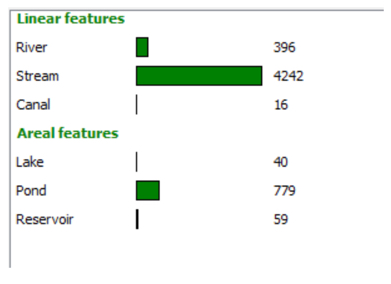
Class hierarchy template file:
If you think you have a good grasp on the fundamentals of object-oriented programming in Python, we recommend that you challenge yourself and try to develop your own solution for this assignment from scratch. However, for the case that you feel a bit overwhelmed by the task of having to implement the class hierarchy yourself, we are here providing a draft file for the waterbody class hierarchy that you can use as a starting point. The file contains templates for the definitions of the classes from the leftmost branch of the hierarchy, so the classes Waterbody, LinearWaterbody and Stream, as well as the ArealWaterbody class. Your first task will then be to understand the definitions and detailed comments, and then add the missing parts needed to complete the definition of the Stream class such as the code for testing whether or not the tag rules for Streams are satisfied, for producing the polyline geometry, and for creating a QgsFeature. The class definition of Stream in particular contains detailed comments on what steps need to be implemented for fromOSMWay(...) and toQgsFeature().
You can then test your implementation by adapting the code examples given above to put together a main program that reads in the data from the JSON input file, calls the fromOSMWay(...) function of the Stream class for each way element, and collects the Stream objects produced from this. You can then either print out the information (name, length) from the instance variables of the Stream objects directly to see whether or not the output makes sense or you next implement the __str__(self) method for Stream to produce the same kind of output with print(result). Then go one step further and write the code for producing a GeoPackage file with the QgsFeature objects produced from calling the toQgsFeature() method for each Stream object that has been created.
Once you have this working for the Stream class, you can start to add the other classes from the hierarchy. You will see that these need to be defined very similarly to the Stream class, so you will only have to make smaller modifications and extensions. Once the full hierarchy is working and you are able to produce the correct GeoPackage files, the final part will be to design and incorporate the GUI.
As a last comment, if you want to make changes to the existing code in the template file, that is absolutely ok; please don't treat it as something that you have to use in exactly this way. There are many possible ways in which this assignment can be solved and this draft follows one particular approach. However, the fromOSMWay(way, allNodes) static class function and toQgsFeature(self) method need to appear in the class definitions with exactly the given paramters, so this is something you are not allowed to change.
Overall, the main.py file and the general file organization of the walkthrough code in Section 4.10 provide a good template for this assignment but no worries, this assignment is significantly simpler and requires much less code. Below you can find two more hints on some of the steps involved.
Hint 1
In the lesson walkthrough, we had a list with the names of all bus event classes that we were looking for in the data. We then used a for-loop to go through that list and call the detect(…) class function for each class in the list. In this assignment, it may make more sense to have two separate lists: one for the class names of the linear waterbody classes and one for the names of the areal waterbody classes. That is because you probably would want to store the objects of both groups in separate lists since they need to be added to two different output files.
Hint 2
If you are using the template class hierarchy file, you won't have to write this code yourself but the following will help you understand what is going on with the length and area computation code: when we have a QgsGeometry object in variable geometry, we can calculate its length/area with the help of an object of the qgis QgsDistanceArea class. We first set up a QgsDistanceArea object suitable for WGS84 coordinates:
qda = qgis.core.QgsDistanceArea()
qda.setEllipsoid('WGS84')
Then we calculate the length or area (depending on whether the geometry is a polyline or polygon) with:
length = qda.measureLength(geometry)
or
area = qda.measureArea(geometry)
Finally, we convert the area or length number into the measurement unit we want, e.g. with
lengthMeters = qda.convertLengthMeasurement(length, qgis.core.QgsUnitTypes.DistanceMeters)
or
areaSquareMeters = qda.convertAreaMeasurement(area, qgis.core.QgsUnitTypes.AreaSquareMeters)
Grading Criteria
The criteria your code submission will be graded on will include how elegant your code is and how well you designed the class hierarchy as well as how well-designed the GUI of your tool is. Successful completion of the above requirements and the write-up discussed below is sufficient to earn 90% of the credit on this project. The remaining 10% is reserved for "over and above" efforts which could include, but are not limited to, the following (the last two options are significantly more difficult and require more work than the first two, so more o&a points will be awarded for these):
- Look through the JSON for some other types of waterbodies (linear or areal ones) that appear there. Pick one and add it to your tool by adding a corresponding class to the waterbody class hierarchy and changing the code so that ways of that class are detected as well.
- Add some code to your tool that first sorts all linear waterbody objects by decreasing length and all areal waterbody objects by decreasing area before adding the objects to the data set. As a result, the order should be as shown in the attribute table images above without first having to sort the rows in QGIS. For this, you should override the < operator by defining the __lt__(self, otherObject) method (for “less than”) for these classes so that it compares the lengths/areas of the two involved objects. You can then simply use the list method sort(…) for a list with all linear/areal objects to do the sorting.
- Add the information display widget showing numbers of objects created for the different classes using QPainter methods to the GUI of your program as described above. The advanced version with bar chart as shown in the image above is sufficient to earn full o&a points if done well.
- Turn the standalone tool into a QGIS plugin that adds the produced data sets as new layers to the project currently open in QGIS using a dock widget as in Section 4.12 (this option alone will give full o&a points if done well).
Write-up
Produce a 400-word write-up on how the assignment went for you; reflect on and briefly discuss the issues and challenges you encountered and what you learned from the assignment. Please also briefly mention what you did for "over and above" points in the write-up.
Deliverable
Submit a single .zip file to the corresponding drop box on Canvas; the zip file should contain:
- The folder with the entire code for your tool
- Your 400-word write-up
Term Project
By this time, you should have submitted your Final Project proposal and received a response from one of your instructors. You have the final two weeks of the course to work on your individual projects. Please submit your agreed-upon deliverables to the Final Project Drop Box by the course end date on the calendar.
There are three parts to the term project submission:
- the documented code and data needed to run it as agreed-upon in the proposal feedback process.
- a write-up describing the project purpose and approach and reflecting on the development and lessons learned from it, as well as providing instructions on how to run and test the code.
- a 5 minute online video demonstrating the project to your classmates and explaining how you realized the project.
More information on these three parts of your term project submission and how they should be submitted can be found below. Please see the project grading rubric on Canvas to understand exactly how these requirements will be evaluated.
Code and data
Deliverable
Submit a single .zip file to the corresponding drop box on Canvas; the zip file should contain:
- Your code and all other files making up your project including the data needed to run and test it
- Your project write-up (see below)
If you are providing any sample dataset larger than about 20 MB, please keep in touch with your grader to ensure that he or she can successfully get the data. You can use your Penn State OneDrive storage here to deliver your data to your grader or alternatively a public service like DropBox, Google Drive, etc., and include the link to your data in your submission. Ideally you can clip your dataset so that it does not take so much space.
Project write-up
Your write-up should discuss the project purpose, how you approached the project and why, and what challenges you had to overcome in the development process. Please make sure you mention packages, libraries, or techniques you used that were not covered in the course materials. Furthermore, you should reflect on what you learned from the project work, how the project could be continued and extended, and things you would do differently next time.
Your write-up should also include a set of numbered steps that graders can follow in order to evaluate your project. If your script or tool requires entering parameters, please provide sample values that the graders could supply for each parameter. If the graders cannot figure out how to run your project, they may deduct functionality points. If your program requires a special environment to be run in or if there are other good reasons why your grader won't be able to run & test out the script (but only then!), you can contact your grader and seek a different arrangement such as demonstrating the script live via Zoom or by recording a more detailed video focussing on running the script. Such alternative arrangements need to be agreed upon before the submission deadline.
Deliverable
Include your write-up in the .zip file with your project code and data (see above) and submit it to the corresponding drop box on Canvas.
Project video
Record a 5 minute demo and discussion video of your project using Kaltura, similar to the video you recorded for part 1 of the Lesson 1 homework assignment. The main purpose of this video is so that everyone can see what the other students did in their projects and potentially learn something from it about APIs we did not cover in the course, techniques, or programming challenges. Therefore, the video should focus on the following points:- Provide an overview on the purpose and motivation for the project
- Demonstrate how the project is applied from a user perspective
- Briefly give an idea of how the code for the project is organized from a programmer perspective
- Pick out two things from your project code that you think would be most interesting for other students and explain them. This can, for instance, be packages, libraries, or techniques you used that were not covered in the course materials or particular challenges you encountered and how you solved them.
Deliverable
Post a link to your video in the Media Gallery.
Please keep in touch with your instructors and fellow students during this time period. I encourage you to help each other in the course forums. It may be that others are encountering the same challenges that you are while working through their projects. Furthermore, I hope you will spend some time after the official end of the class to check out the video presentations of your classmates and provide comments and feedback in the Media Gallery. Surely, there will be many new insights and ideas to be gained from these videos.
This course has been a pleasure and I wish you the best in your future Python and programming endeavors!