GEOG 863
Lesson 1: Creating Mapping Apps Without Programming
Overview
Overview
In this course, we'll be spending the bulk of our time learning how GIS web applications can be built using a mapping Application Programming Interface (API) created by Esri in combination with the core web development technologies of HTML, CSS, and JavaScript. However, before digging into those programming languages and that API, it's worth noting that Esri also provides non-programming tools for creating mapping apps. These tools don't provide the same level of control over the final product as one developed using code written on top of the API, but they might meet some of your app development needs. And as we'll see later in the course, a smart workflow is to use tools in ArcGIS Online to handle certain parts of the app development (layer symbology, popup window content, etc.) and develop the rest of the app through coding.
Objectives
At the successful completion of this lesson, you should be able to:
- overlay your own data on top of an Esri basemap using ArcGIS Online;
- embed your maps within a web page;
- build applications around your maps (providing greater interactivity and functionality) through the use of development tools from Esri.
Questions?
Conversation and comments in this course will take place within the course discussion forums. If you have any questions now or at any point during this week, please feel free to post them to the Lesson 1 Discussion Forum. (That forum can be accessed at any time by clicking on the Discussions tab.)
Checklist
Checklist
Lesson 1 is one week in length. (See the Calendar in Canvas for specific due dates.) To finish this lesson, you must complete the activities listed below. You may find it useful to print this page out first so that you can follow along with the directions.
| Step | Activity | Access/Directions |
|---|---|---|
| 1 | Work through Lesson 1. | Lesson 1 |
| 2 | Create a mapping app of your own choosing using Esri's Web AppBuilder or one of their configurable templates. | Post a link to your app in the Lesson 1 Discussion Forum. |
| 3 | Review another web mapping platform. | Post a link to your video review in the Lesson 1 Discussion Forum. |
| 4 | Take the Lesson 1 Quiz after you read the course content. | Click on "Lesson 1 Quiz" to begin the quiz. |
1.1 Building a Web Map (Map Viewer)
1.1 Building a Web Map
Several GIS technology vendors provide the means for non-programmers to create web maps without writing any code (e.g., Google's My Maps, CartoDB, ArcGIS Online), and the capabilities of these map authoring applications are increasing constantly. In this part of the lesson, we will explore Esri's ArcGIS Online (which I'll abbreviate as AGO hereafter).
- Follow this link to the Penn State home page at AGO. You'll need to authenticate through Penn State WebAccess if you haven't already today. Once logged in, you should see the Home tab selected for the Penn State organizational account.
If you completed GEOG 483, your first hands-on GIS project involved helping "Jen and Barry" find the best place to open an ice cream shop in a parallel universe where the cities and counties of Pennsylvania have different names. We're going to work with the data from that scenario again here (and later in the course), since it contains examples of each geometry type and some good attribute data for demonstration purposes.
- Download and unzip the Jen and Barry's data. (Even if you still have these shapefiles from an earlier course, you may want to download this copy since the shapefiles are zipped and ready for upload to AGO.)
This zip file contains a point shapefile (cities), a line shapefile (interstates) and two polygon shapefiles (recareas and counties). You can check out these shapefiles if you haven't encountered this scenario before, but hang on to the zip files since we'll be uploading them to AGO.
We're going to build a web map containing the Jen and Barry's data. The old Map Viewer made it possible to add a shapefile directly to the map, and for a while the new one did not but that functionality as been re-introduced. So we'll begin by creating hosted feature layers from the shapefiles you downloaded.
- Click on the Content tab, then on the New Item button in the upper left.
- Drag and drop the zipped cities shapefiles onto the large box that takes up the top half of the New Item dialog.
- AGO should recognize the contents of the zip as a shapefile. Accept the default option to both upload the data and create a hosted feature layer, then click Next.
- Assign a Title to the layer -- it should default to match that of the shapefile, though you're welcome to give it a different name. You can also specify a folder, tags, and a summary, if you wish. Click Save when done.
When the data has been uploaded, you should see a page of details about your new feature layer along with a number of buttons running down the right side of the page. In a real-world project, it would be a good idea to fill out the metadata on this page, especially the items marked REQUIRED.
- Click the top Open in Map Viewer button to add the data to a new web map.
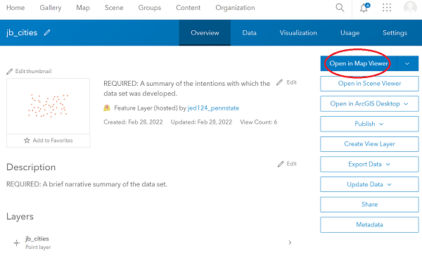
Figure 1.1 Opening a feature layer in the AGO Map Viewer
- AGO will display the cities using a single symbol by default. To modify the symbology, click on the name of your layer within the Layers panel or click the Options (3 dots) button followed by Show properties. The right side of the map should change to display various properties of your layer, in categories such as Information, Symbology, Appearance, etc.
Speaking of the "3 dots" button, note that this menu is where you'd go if you wanted to view the layer's attribute table or remove the layer from the map, among other options.
As in desktop software, you can create a thematic styling of your data in AGO. For example, you might choose to symbolize the Jen and Barry's cities based on the POPULATION field, selecting a style of Colors and Amounts (size) or Colors and Amounts (color). We won't do that here, instead sticking with the Location (single symbol) style, but let's modify that symbol.
- Expand the Symbology property group, if necessary, and click on Edit layer style.
- Next, click on Style Options, then click on the current symbol that was assigned by default. A panel of symbol properties should pop out on the left of the symbol.
Note that through this panel, you can choose from several symbol categories (Basic Shapes, Firefly, Government, etc.). You can also customize a number of other properties, such as size, rotation, transparency, fill color, and the symbol outline.
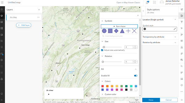
Figure 1.2 Changing layer symbology in AGO
- Select any icon that grabs you.
- To apply your change and wrap up your work with the layer's properties, click the X in the upper right of the symbol options panel, then click Done twice.
We're next going to add the other Jen and Barry's data, but first we should save this web map.
- About halfway down the black strip of buttons on the left side of the window, you should see a folder icon with a blue dot over it. (The blue dot indicates you have unsaved changes in this map.) Click this button, then on Save as.
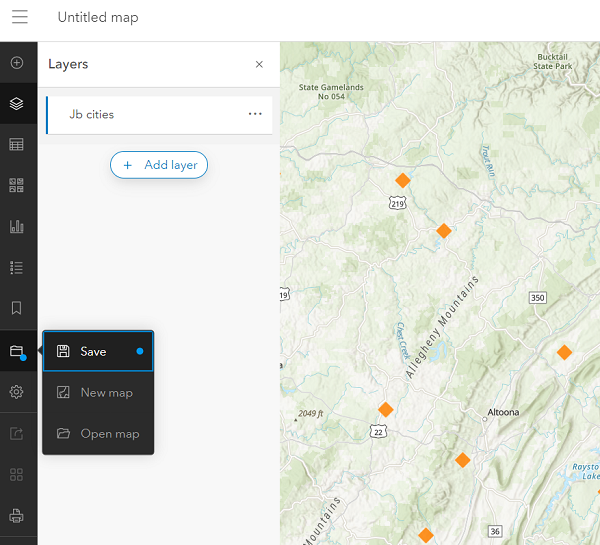
Figure 1.3 Saving the web map
- In the resulting Save map dialog, assign a Title of Jen and Barry - <your name or ID>. Optionally, add some tags and a summary, or change the folder where the map will be saved.
- Click Save map when finished. You should now see the title you assigned in the upper left of the window.
To add the interstates data, we need to import it to AGO through the Content tab as we did earlier for the cities.
- Return to the Content tab by clicking on the "hamburger" icon in the upper left of the window and choosing Content.
- Follow the steps used earlier to create hosted feature layers in your account from the interstates and counties shapefiles. You're welcome to also import the recareas, though you won't be asked to work with them in this walkthrough.
- Re-open the web map you saved earlier by returning to the Content tab, clicking on your web map and selecting Open in Map Viewer from its details page.
- On the Layers panel, click Add. You should be presented a list of layers in your AGO account.
- Locate your interstates layer and add it to the map by clicking the +Add button associated with that layer.
Let's symbolize this layer using values from its TYPE field.
- The layer's style settings should already be visible in the properties panel on the right side of the map. Under Choose Attributes, click the + Field button.
- Select the TYPE field, then click Add. Note that AGO intelligently applies the Unique symbols drawing style (based on the field holding text strings rather than numbers).
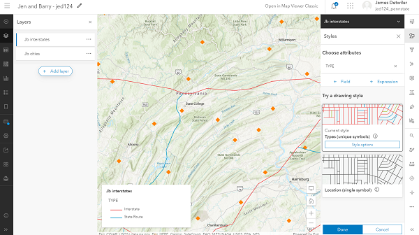
Figure 1.4 Displaying interstates by type - Click Style options. You should see a separate symbol for each of the two unique values in the TYPE field: State Route, Interstate, and Other.
- Modify the symbols to your liking. (A thicker line is intuitive for the Interstate features, a setting that can be made by changing the Width property.)
- Again, click X and Done twice when you're finished symbolizing the interstates layer.
- Following the same sort of procedure, add the counties layer to the map and set its symbology so that the county features are drawn using a hollow fill. (Polygon layers are symbolized with a fill color by default, but that can be disabled by clicking the No color button under the Fill Color heading.) You may also want to modify the outline properties.
Next, let's explore the pop-up windows that appear when the user clicks on a map feature.
- Click on one of the cities features to bring up a pop-up window.
Because the cities features overlap counties features, the pop-up results will include features from both layers. You should see text at the top of the window like "1 of 2" or "1 of 3" indicating this.
- Click on the right arrow to cycle through the pop-up results and note that the matching feature is highlighted on the map.
There are a number of improvements that could be made to the information displayed in this pop-up.
- Display the properties of the cities layer as you did earlier. It will probably default to showing the drawing styles.
- In the strip of buttons running along the right side of the window, click Pop-ups.
Values from columns in the layer's attribute table are displayed in the pop-up by enclosing the column within braces. Thus, the pop-up Title is set to display the value from the layer's NAME column using the expression {NAME}.
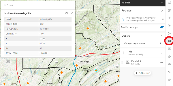
Figure 1.5 Configuring pop-ups
All of the layer's fields -- with the exception of FID -- will be included in the pop-up by default, but this can be customized.
- Click on Fields list, then on the x beside the ID, X, and Y fields, to exclude those fields from the pop-up content. Note that the pop-up that appears over the map is updated dynamically in response to your modifications.
- It's possible that the fields won't be listed in a logical order. Clicking on the 6 dots just to the left of the field name, click and drag the fields as necessary to order them as follows: NAME, POPULATION, UNIVERSITY, TOTAL_CRIM, CRIME_INDE.
There are other settings that can be applied to make the pop-up more human friendly. For example, some of the field names are abbreviated and/or include underscores. And the numeric fields display two digits after the decimal point, but that is meaningless for those fields.
- Looking again at the strip of buttons along the right, click on the Configure Fields button (one below the Popups button).
- Click on the TOTAL_CRIM field and in the panel that appears to the left, give it a new Display name and set the Significant digits property to 0 decimal places. Click Done to dismiss this panel.
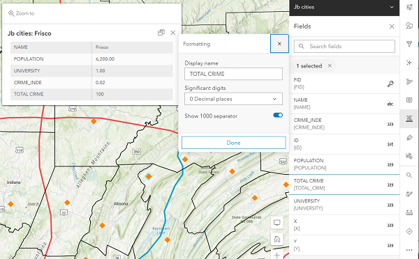
Figure 1.6 Making the pop-ups more user-friendly
Following a similar process, make similar improvements to other fields as appropriate. - Once done modifying the layer's settings, click on its entry in the Layers panel to toggle off its properties panel.
Test your changes by clicking once again on a cities feature.
Note that it is possible to customize pop-ups further (e.g., to string together values from multiple columns) or to display media such as images and charts.
Challenge → The UNIVERSITY field holds a 1 for cities that have a university and a 0 for cities that do not. This would be a bit more human-friendly if it displayed as Yes/No (or True/False). If you can work out how to implement such a change, feel free to share your solution in the Lesson 1 Discussion Forum.
We can also choose to utilize a different base map.
- In the strip of buttons running down the left side of the window, click on the Basemap button and choose one of the options. (A light base map is often preferable to a dark one, since your layers will stand out better.)
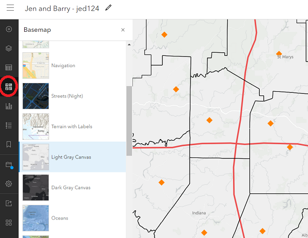
Figure 1.7 Changing the basemap
- Be sure to Save the changes you've made to your web map.
- Finally, make your map visible to others by clicking Share map (also on the left-hand toolbar).
- Set the map's visibility to Everyone (public), as we'll be embedding this map in a web page in a moment, then click Save.
Unless you also made the map's layers public -- the walkthrough didn't tell you to -- you should see a dialog warning you that they won't be visible, but also giving you a chance to rectify that.
- Click the Update sharing button to set sharing on the layers to public as well.
- To confirm that others will be able to see your map, try opening the URL in another browser (e.g., use Edge if you're currently working in Chrome).
In this section, we've been able to build a useful interactive web map without any programming. Move on to the next page to see how to take your ArcGIS Online map further -- still without programming -- by embedding it within a web page and using it as the basis for a web application.
1.1 Building a Web Map (Map Viewer Classic)
Note: This page walks through creation of the same web map as the previous page, just with the "Classic" version of the ArcGIS Online Map Viewer. You're welcome to skip over this page if you've already completed the Jen and Barry's web map on the previous page.
1.1 Building a Web Map
Several GIS technology vendors provide the means for non-programmers to create web maps without writing any code (e.g., Google's My Maps, CartoDB, ArcGIS Online), and the capabilities of these map authoring applications are increasing constantly. In this part of the lesson, we will explore Esri's ArcGIS Online.
- Go to the Penn State home page at ArcGIS Online and click the Penn State WebAccess button to authenticate.
- Click on Map to begin work on a new map. If this opens some other map you've worked on previously, select New Map (top right) to start with a clean slate.
If you completed GEOG 483, your first hands-on GIS project involved helping "Jen and Barry" find the best place to open an ice cream shop in a parallel universe where the cities and counties of Pennsylvania have different names. We're going to work with the data from that scenario again here (and later in the course), since it contains examples of each geometry type and some good attribute data for demonstration purposes.
- Download and unzip the Jen and Barry's data. (Even if you still have these shapefiles from an earlier course, you may want to download this copy since the shapefiles are zipped and ready for upload to ArcGIS Online.)
This zip file contains a point shapefile (cities), a line shapefile (interstates) and two polygon shapefiles (recareas and counties). You can check out these shapefiles if you haven't encountered this scenario before, but hang on to the zip files since we'll be uploading them to ArcGIS Online.
- In ArcGIS Online, click the Add menu, then select Add Layer from File.
As explained in the dialog, this option enables you to upload zipped shapefiles, delimited text files, and GPX (GPS interchange) files. Note the other options for adding data in this menu. We'll use them later.
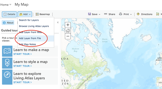 Figure 1.1 The Add Layer from File option in ArcGIS Online
- Click the Browse button, then navigate to your copy of the Jen and Barry's cities zip file.
- Accept the default Generalize features option.
We're importing these data purely for display purposes, so it makes sense to take advantage of the improved drawing speed that generalization provides. If we were conducting analysis that relied on highly accurate feature geometries, we would select the Keep original features option instead.
- Click Import Layer to complete the upload process.
ArcGIS Online will automatically get you started symbolizing your data by providing a two-step dialog for styling the cities layer. The first step involves selecting an attribute to show, while the second presents drawing style options based on the selection made in the first step.
By default, the layer is shown as graduated symbols based on the POPULATION column using the "Counts and Amounts (Size)" option. Note that symbolizing the cities with a color ramp would be done using the "Counts and Amounts (Color)" option. Let's change the display of the cities so that they are all drawn with the same symbol.
- Under Choose an attribute to show, select Show location only.
- Under Select a drawing style, default is Location (single symbol), select OPTIONS.
We'll change the symbol used for the cities in a moment, but first notice that it is possible to set the transparency and the scale range at which the layer is visible on this panel.
- Click Symbols.
Select any icon that grabs you. Note that there are a number of icon categories, that it is possible to customize the icon's size, and that you can also use your own image as the icon.
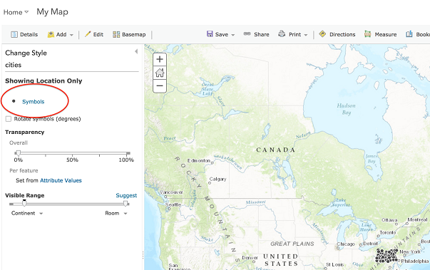 Figure 1.2 Changing layer symbology in ArcGIS Online
- Click OK to dismiss the symbology options and DONE to finish modifying the cities layer. You should see the cities layer listed under the Contents heading of the Details panel.
- Note the buttons that appear beneath the layer name, allowing you to see the layer's legend, open its attribute table, change the layer's style, perform analysis, and access a host of other miscellaneous options.
- Return to the Add Layer from File dialog and add the interstates shapefile as a layer. Again, ArcGIS Online will immediately launch into styling the new layer.
- Choose TYPE as the attribute to show and note that ArcGIS Online intelligently applies the Unique symbols drawing style (based on the field holding text strings rather than numbers).
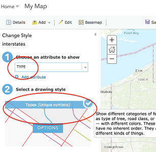 Figure 1.3 Symbolizing by an attribute in ArcGIS Online
 - Click OPTIONS. You should see a separate symbol for each of the two unique values in the TYPE field: State Route, Interstate, and Other.
- Modify the symbols to your liking. (A thicker line is intuitive for the Interstate features.)
- Again, click OK and DONE to return to the Details panel when you're finished symbolizing the interstates layer.
- Following the same sort of procedure, set the symbology of the counties layer so that the county features are drawn using a hollow fill. (Under the color palette is an empty square with a red line through it, which is used to specify "No color.") You may also want to create a darker outline color.
Next, let's explore the pop-up windows that appear when the user clicks on a map feature.
- Click on one of the cities features to bring up a pop-up window.
Because the cities features overlap counties features, the pop-up results will include features from both layers. You should see text at the top of the window like "1 of 2" or "1 of 3" indicating this.
- Click on the right arrow to cycle through the pop-up results and note that the matching feature is highlighted on the map.
There are a number of improvements that could be made to the information displayed in this pop-up.
- Click on More Options (3 dots) next to the cities layer and select Configure Pop-up.
Values from columns in the layer's attribute table are displayed in the pop-up by enclosing the column within braces. Thus, the Pop-up Title is set to display the value from the layer's NAME column using the expression {NAME}.
- Click on the Configure Attributes link just below the list of fields.
The dialog contains two sets of checkboxes: one for specifying which fields will be displayed and another for specifying which can be edited. Note that the checkbox in the header itself can be used to toggle all fields on/off.
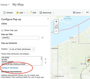 Figure 1.4 Configuring attributes in ArcGIS Online
- Editing capability isn't needed, so uncheck Edit for all fields.
- Under Display, uncheck the checkboxes next to the FID, ID, X and Y fields to exclude those values from the pop-up content.
- Click on the TOTAL_CRIM field alias and give it a new alias that makes the pop-up more human friendly. Do the same for CRIME_INDE.
The POPULATION, TOTAL_CRIM and UNIVERSITY values display with two digits after the decimal point, but that is meaningless for those fields.
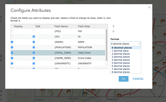 Figure 1.5 Assigning user-friendly field aliases in ArcGIS Online
- Click on the {POPULATION} field, then change the Format option from 2 decimal places to 0 decimal places. Do the same for {TOTAL_CRIM} and {UNIVERSITY}.
- Click OK to dismiss the Configure Attributes dialog, then OK again to save your pop-up changes.
Test your changes by clicking once again on a cities feature.
Note that it is possible to customize pop-ups further (e.g., to string together values from multiple columns) or to display media such as images and charts. It's also possible to utilize a different base map.
- Click on the Basemap button and choose one of the options. (A light base map is often preferable to a dark one, since your layers will stand out better.)
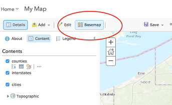 Figure 1.6 Changing the basemap in ArcGIS Online
 - Save your work by going to Save > Save As.
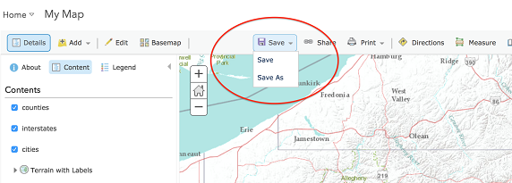 Figure 1.7 Saving a map in ArcGIS Online
 - To make it easy for me to find your map, please give it a Title of Jen and Barry - <your name>.
- Enter a logical Tag or two (e.g., GEOG 863) and an appropriate Summary (e.g., A map for GEOG 863, Project 1), then click SAVE MAP.
- Finally, make your map visible to others by clicking Share.
- Set the map's visibility to Everyone (public), as we'll be embedding this map in a web page in a moment.
- To confirm that others will be able to see your map, try opening the URL in another browser (e.g., use Chrome if you're currently working in Firefox).
In this section, we've been able to build a useful interactive web map without any programming. Move on to the next page to see how to take your ArcGIS Online map further -- still without programming -- by embedding it within a web page and using it as the basis for a web application.
1.2 Turning Your Map into an App
1.2 Turning Your Map into an App
The map created earlier in the lesson offers interactivity in the form of zooming in/out, toggling layers on/off, accessing information about map features by clicking on them, changing the base map, etc. This part of the lesson will begin by showing you how to embed your map within a separate web page. After that, we'll look at tools developed by Esri that make it possible to incorporate even more interactivity -- to turn your map into an app.
1.2.1 Embedding a Map
1.2.1 Embedding a Map
While it's sometimes preferable to share the link to your map -- allowing it to fill the viewer's browser window -- it can also be useful to embed the map within a web page.
- Save this example page to your computer. (Right-click on the link and choose Save.)
- Open the page in a plain text editor of your choosing (e.g., Notepad).
- If your ArcGIS Online map is no longer open, go to our Penn State organization page, click the Content tab, and click on the map you created earlier.
What we're about to do is not (yet?) supported by the current Map Viewer, so rather than click on the Open in Map Viewer button, click instead on the dropdown arrow just to its right and select Open in Map Viewer Classic.
- Click Share, then EMBED IN WEBSITE.
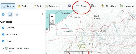 Figure 1.8 Opening the dialog for embedding a map in a website
Note that AGO provides a number of options for customizing the embedded map. For example, it's possible to specify the dimensions of the map, and to include widgets such as a base map selector or legend.
- After making settings to your liking, find the wide text box just above the Map Options. This box contains the HTML code required to embed your map within a web page. Click the COPY button to the right of that text box to copy the HTML code to your machine's clipboard.
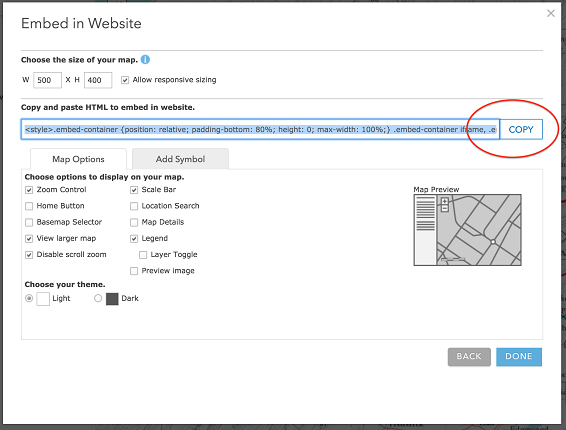 Figure 1.9 Copying the code for embedding a map in a website
 - Paste that code into your HTML document just beneath the My ArcGIS Online Map heading. Double-check the URL to your map. If it doesn't include the http: protocol, you will need to add it in front of //pennstate.maps.arcgis.com in the html code for your map to connect properly.
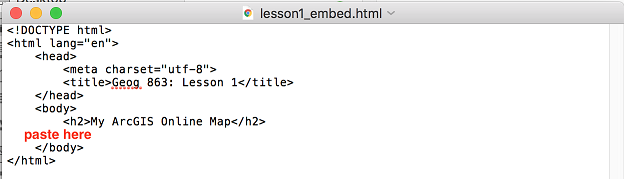 Figure 1.10 Pasting code to embed a map in a website
 - Save your HTML document with a name like lesson1.html.
- Using the File Explorer in Windows, browse to the document you just saved and double-click on it to open it in a web browser. (If .html files aren't set to open in a web browser on your machine, you may need to right-click and select Open With.)
- If you get an error that your map cannot be loaded or found (a blank grey box under your title), go back into your HTML file and add http: before //pennstate.maps.arcgis (etc.). so that it looks like:
http://pennstate.maps.arcgis.com/apps/Embed......
1.2.2 Configuring an App Based on a Template
1.2.2 Configuring an App Based on a Template
The interactivity offered by this map is nice, but you may find yourself in situations where you need to go further. For example, maybe you want end users to be able to query the map's underlying data for features meeting certain criteria or to be able to edit the underlying data. Esri offers a couple of different non-programming options for those looking to build apps with greater functionality. The first of these is a set of templates that each meet a narrowly focused need (e.g., Basic, Nearby, Sidebar). As the app developer, you select the desired template and make a relatively small number of configurations to tailor the app to your needs. The second option is to use Web AppBuilder. This option is more open-ended, allowing you to build a less narrowly focused app by picking and choosing from a set of widgets.
We'll start with configurable app templates and to demonstrate their use we'll create an app for locating buildings on the Penn State Main Campus.
 As with the Map Viewer, Esri has an older set of configurable app templates and a newer one (which they've branded as Instant Apps). In this walkthrough, I'd like to show you how to include a logo and an opening splash screen in your app. It turns out that building such features into an Instant App is more difficult to do. A logo can only come from an organization-level shared theme setting and I don't see a splash screen option (though some Instant Apps templates offer a Details panel that can serve a similar purpose). So in this section, you'll be led through creating an app with an older template (with the logo and splash screen) and in the next section you'll see how a similar app can be built with one of the newer Instant Apps templates.
- In your Penn State ArcGIS Online organizational account, create a new map. Be sure to switch to Map Viewer Classic.
- Add the campus building data as a layer by going to Add > Add Layer from Web and pasting this ArcGIS Server map service:
https://mapservices.pasda.psu.edu/server/rest/services/pasda/PSU_Campus/...
Notice that the ArcGIS Services are the default, but the dropdown menu allows you to add several other types of online data. - Zoom to the central part of campus and style the layer as desired.
- Save the map with the name PSU Buildings. Be sure to add some tags that would aid in discovering the map (e.g., Penn State, buildings) and optionally enter a summary.
- Click Share, then check the Everyone box to ensure your map is viewable to the public.
- Click Create a Web App.
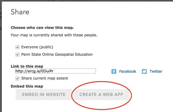 Figure 1.11 Accessing the app template options in ArcGIS Online
You'll be presented with a gallery of app templates on which you can base your own app. The gallery will default to Use Instant Apps under What do you want to do?, but you can see the older templates by choosing Show All. Browse the templates to get a sense of the variety of apps available.
We're going to create a Basic Viewer application and configure it so that users can search for buildings by name. - Click on the Basic Viewer template and select CREATE WEB APP. Note: You'll also see an Instant App template by the name of Basic, but be sure you choose Basic Viewer.
- Assign a title to the app (e.g., Penn State Main Campus Building Finder), add some tags that would aid in discovering the app (e.g., Penn State, buildings), optionally enter a summary, then click DONE. After a few moments, you'll be presented with a Configure page. The full set of configuration options for this template are organized under the tabs General, Theme, Options and Search. Let's start with the General tab, already shown by default.
- The app preview on the right initializes with a heading based on the underlying map name. Change this by setting the Application title to Penn State Main Campus Building Finder.
Other options under the General tab have to do with providing some background info to the user regarding the app's purpose and/or use. This can be done through a Details dialog or through a Splash Screen. Both options offer a WYSIWYG HTML editor for defining the content. The main difference is that the splash screen appears automatically when the app loads (but cannot be viewed after that), while the Details dialog can be opened whenever desired via a button. Some apps require no background info, while others are not as intuitive. You may choose to employ neither, just one, or both of these options, depending on the app.
For this app, let's go with a Splash Screen, but no Details. - Check the Splash Screen checkbox, then set the properties as follows:
Splash screen title: Welcome!
Splash screen content text: Enter a text string in the search box to find all buildings containing your search string.
Define custom button text: Close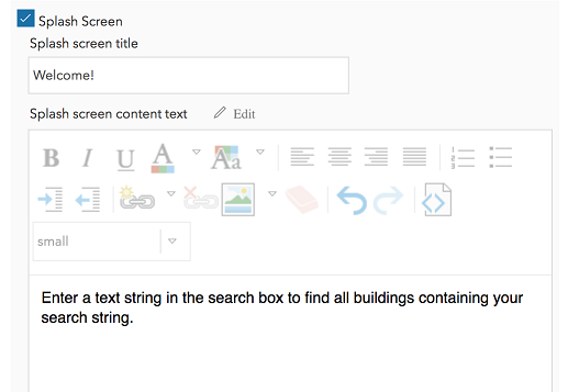 Figure 1.12 Defining Splash Screen properties in the Basic Viewer configurable app
 - Click Save to save your configurations so far and refresh the webpage. When the app preview reloads, you should see the changes you've made, including the splash screen.
- Now, move to the Theme tab and set the Title logo to http://www.e-education.psu.edu/geog863/sites/www.e-education.psu.edu.geog863/files/psu-facebook-avatar-180x180.jpg and the Logo link to http://www.psu.edu. Note that while the image is actually 180 pixels x 180 pixels, it will be dynamically resized to 48 pixels x 48 pixels.
- Feel free to experiment with the layout options. (You'll need to click Save to refresh the preview after selecting a different layout.) I'm partial to the Default, but you're welcome to choose a different one.
At the top of the Theme tab, you have the ability to customize the colors of the header background, header text, button icons, panel background and panel text. It turns out that Penn State's blue and white colors are already a pretty good match for the app's default colors. However, we can adjust the header background color to match the Penn State blue a bit better. - Open the Penn State shield used above in Firefox, then right-click on the image and choose Inspect Element. (Guidance on doing the next step in Chrome can be found beneath the figure below.)
- Under the Inspector tab, you should see an eyedropper icon. If you've worked in image editors like Photoshop, you should be familiar with how this tool works. Click on the tool to activate it, then click on the blue part of the shield. This will copy the hexadecimal value of that color to your clipboard. (The shield contains many shades of blue, so your color value is likely to be different from mine.)
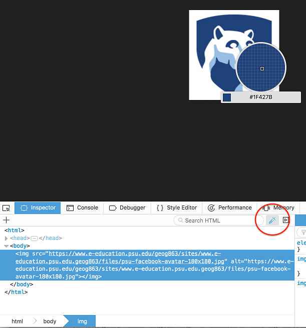 Figure 1.13 Using the browser's color picker
If you'd prefer to do this in Chrome, you should be able to access a similar tool by right-clicking on the image > Inspect; under the Styles tab, click the colored square next to the background-color property. The color picker dialog that appears contains an eyedropper tool. Click to select it, then click in the blue of the image as described above. That blue color will then be selected in the color picker. The dialog shows color values in the HSLA specification scheme by default; if you click the double-arrow button to the right of the color values, you can view the color in other specification schemes, including its hexadecimal (HEX) value.
- Return to the app and Paste the copied color value in to set the Header color property.
- Move to the Options tab and spend a few minutes examining the many ways you can customize the app GUI. Here are the settings I would make for this app:
- Display scalebar on map
- Turn off Bookmarks. (I didn't see a tool associated with this option on the GUI anyway and this option may not even be available to you.)
- Turn off Map Details. We left this option empty under the General tab earlier, opting to show a splash screen only.
- Turn on the Measure tool. You should experiment with this; it can be used to measure lengths and areas.
- Uncheck Display layer list. There's not much point in letting the user toggle the buildings on/off in this app.
The Basic Viewer template provides a box for the user to enter search text, which by default is set to work against Esri's world geocoder. We'll now carry out the most important of our customizations by wiring up the search box to a column in the buildings layer that holds the building names. - Click the Search tab, uncheck the Esri World Geocoder option and check the PSU Buildings option.
- Click the Edit button next to the PSU Buildings option.
- From the Search Fields list, select BLDG_NAME_.
- Set the Placeholder to Enter part of a building name.
- Check the Enable Suggestions box. This will find matches in the buildings layer and present them in a dropdown list as the user types.
With that, you've made all the necessary settings to tailor this template to your specific purpose. - Click Save and Close once you're satisfied with the app's settings. You'll be taken to your app's "item details" page (also accessible from your "My Content" page).
- To see the app as an end user would see it, click the View Application or Launch button to open it in a new browser tab.
- Test your new app by entering the name 'walker' in the search box. You should see that the app finds three buildings that make up the Walker Clubhouse (associated with the PSU golf courses), Walker Building (home of the Geography and Meteorology departments) and a bus shelter near Walker Building. Note how the settings you made when configuring are reflected in the app.
- Returning to the Details page for our app (visible by clicking on your map/app from "Content" under "Home" in ArcGIS Online) , note the various pieces of metadata that can be edited (thumbnail, description, access use and constraints, etc.).
- Note also that you would come here and click the Configure App button if you wanted to make changes to the app.
- Finally, and importantly, if you want others to be able to use your app, you'll need to click the Share button. In the Share dialog, you can select whether you want the app to be visible to Everyone, your Penn State group, or some other group to which you belong. Select Everyone in this case.
- And just to test your app's visibility, scroll to the bottom of the app's Details page and find the URL in the bottom right. Click the Copy button to copy the URL to your clipboard, then paste that URL into a different browser where you are not signed in to ArcGIS Online. If the app works properly, then you can safely share that URL with your end users.
Remember that there are many configurable app templates available to you as an app developer. Often there are multiple templates that can serve as logical starting points, and depending on the widgets employed by the template, you'll see different customization options.
1.2.2 Configuring an App Based on a Template (Instant Apps)
1.2.2 Configuring an App Based on a Template (Instant Apps)
Now let's see how a similar app can be built using one of the newer Instant Apps templates. (You can skip steps 1-5 if you already created and saved a PSU Buildings web map in the previous section.)
- In your Penn State AGOL organizational account, open a new Map, sticking with the current Map Viewer.
- Add the campus building data as a layer by clicking Add > Web service and pasting this ArcGIS Server map service:
https://mapservices.pasda.psu.edu/server/rest/services/pasda/PSU_Campus/... - Zoom to the central part of campus and style the layer as desired.
- Save the map with the name PSU Buildings. Be sure to add some tags that would aid in discovering the map (e.g., Penn State, buildings) and optionally enter a summary.
- Click Share map, then check the Everyone box to ensure your map is viewable to the public.
- Click Create app. (It's the button below Share map.)
You'll be presented with a gallery of app templates on which you can base your own app. Browse the templates to get a sense of the variety of apps available. Note that how your map will look within a given template can be previewed by clicking on the desired template and selecting Preview.
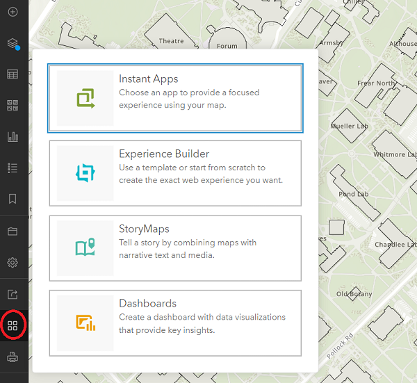 Figure 1.14 Creating an Instant App
We're going to create a Sidebar application and configure it so that users can search for buildings by name. The Basic template would be appropriate too, though it doesn't appear to offer a way of displaying the usage instructions that we showed through a splash screen in the previous app. - Locate the Sidebar template and click Choose.
- Assign a title to the app (e.g., Penn State Main Campus Building Finder Instant App), add some tags that would aid in discovering the app (e.g., Penn State, buildings), optionally enter a summary, then click Create App. After a few moments, you'll be presented with a page for Configuring the app. The app configuration process defaults to an Express mode, which presents a set of essential settings to consider in five categories.
If it's your first time with Instant Apps, you'll be presented with a dialog of tips before you can begin configuring. - Read over the tips, clicking Next to move from one to the next, then Done when you've read the last tip.
- Go to the Step 1 settings and note that the Map is already selected. This makes sense as you just chose to create an app from the Map Viewer, but you'd have the ability here to select a different map if you wanted.
- Click Step 2. About to move on to Step 2, which involves providing info that will help the user understand the purpose behind your app.
- Confirm the Header is toggled on and set the App title to Penn State Main Campus Building Finder.
The Step 2 settings offer one way to provide user instructions through an Introduction window. This adds an I icon to the map that the user can click on to get info on the map's purpose and/or instructions. Unfortunately, it can't be set to open when the app loads. There is another option that I like a bit better, so leave the Introduction panel toggled off. - Click Next to move on to Step 3.
- A legend is probably not necessary in this scenario, so toggle the Legend option off.
- Displaying info on selected buildings in a side panel is a nice feature, so leave the Pop-up panel toggled on.
- The Details panel should be enabled by default. It is the other way to provide user instructions. Edit its content to appear as follows:
Welcome! Enter a text string in the search box to find all buildings containing your search string.
Specify that it should also be open by setting the Select which panel to open at start option (top of the Step 3 settings) to Details. - Click Next again to move on to Step 4, which presents a number of interactivity settings. Take a moment to look over the available options, clicking on their info buttons if you're unsure what they mean.
The goal of this app is to provide the user with the ability to find a building by name, so we want the Search widget to be enabled. (It is by default.) However, its default behavior is to pass the entered text to the ArcGIS World Geocoding Service, which is not what we're looking for. Let's configure the app to use the buildings layer from the map as a Search source. - Under the ArcGIS World Geocoding Service source, click Add a source. You should be presented with options for specifying a layer source from a URL or from the map.
- Choose Map. In this case, the map contains just a single layer, which you should see listed.
- Click on that buildings layer to select it.
- Set the Layer Name to PSU Campus Buildings.
- We could set the Placeholder text to something more context-specific, but it would only appear if we were going to allow the user to select from multiple search sources (which we won't be doing). So leave this setting unchanged.
- From the Search field dropdown list, select BLDG_NAME_ . Note that you could add other fields to search as well, if desired.
- Click Done to complete the addition of the new source for the Search widget. You should now see both the geocoding service and the buildings listed as sources.
- As we don't really need to support geocoding, click on the three dots next to the Geocoding Service source, then click Delete.
- Finally, confirm that the Search open at start option is toggled on.
- Click Next to move on to the last group of settings, which control the theme and layout of the app's widgets. We'll leave these settings on their defaults, but note that we could choose a Light or Dark theme and move the widgets (a Home button, Zoom controls, the Search widget, and a Scalebar widget) to different positions.
- Click Publish and then Confirm to complete the configuration of the app.
After a few moments, you should be presented with a dialog containing some sharing options. Note that the app is not shared with the public by default. You have the ability to change that here if you wish. You'll also see buttons for sharing through social media and code that you could copy if you wanted to embed the app in a webpage like we embedded a web map earlier in the lesson.
- Click Launch to have a look at your app as an end user would see it.
The Details panel should be open on load, showing the user instructions.
- Try testing the search box (e.g., for Pattee Library) to confirm that it's working properly.
Now that you've seen how to quickly put together an app using a couple of different configurable templates, let's have a look at an option that provides a bit more flexibility.
1.2.3 Creating an App with the Web AppBuilder
1.2.3 Creating an App with the Web AppBuilder
Now let's try one of Esri's more open-ended options for creating apps, the Web AppBuilder.
- Re-open your Buildings map using Map Viewer Classic and click again on the Share button.
- Click Create a Web App and this time click on the Web AppBuilder tab rather than the Configurable Apps tab.
- Assign a Title of PSU Main Campus Buildings, add some tags that would aid in discovering the app (e.g., Penn State, buildings), optionally enter a summary, then click Get Started.
The Web AppBuilder will open with configuration options organized within tabs on the left side of the window and a preview of your new app on the right side. The app is dynamically linked to the configuration options so that changes made on the left will be reflected on the right immediately. The first of the configuration tabs is Theme, which provides access to settings that deal mainly with the app's appearance.
- Try out some or all of the available themes (Billboard, Box, Dart, etc.). The controls on the app preview are functional, so you can click on the Legend and Layer List controls to see how they would behave. Depending on the theme chosen, you will see different options under the Style and Layout headings.
- Click on the Map tab and note that it is possible to change the app's underlying Web Map and to override the map's initial extent and visible scale levels.
- Next, click on the Widget tab. This is where the real power of the Web AppBuilder becomes apparent.
The widgets available in Web AppBuilder can be categorized as off-panel or in-panel. Off-panel widgets are built into the app and can only be toggled on/off. Examples include the Scalebar and Coordinate widgets. In-panel widgets, on the other hand, can be added to or removed from the app. When adding an in-panel widget, the developer can position the widget within a container. If you experimented with the various themes, you saw that the shape and positioning of the widget container is something that differs across the themes. And for some themes, in-panel widgets can also be placed in numbered positions outside of the theme's container.
- Hover your mouse over some of the off-panel widgets and note the following:
- An eye icon appears in the widget's upper-right corner. The widget can be toggled on/off by clicking on this icon. Widgets that have been turned on are shaded dark blue, while those that are turned off are light blue.
- Widgets that are toggled on will have their position within the app highlighted in red.
- A pencil icon appears in the widget's lower-right corner. The widget can be configured by clicking on this icon. (For example, the Scalebar widget can be configured to show distance measured in English units, metric units, or both.)
- Turn on the following widgets: Attribute Table, Coordinate, My Location, Scalebar, Overview Map (you'll probably need to be using the Box theme for these).
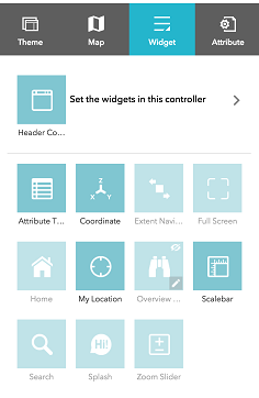 Figure 1.15 Choosing widgets in Web AppBuilder
 - Configure the widgets as follows:
- Attach the Overview Map to the top-right corner and initialize it in its expanded state.
- Modify the Attribute Table so that only the building name and abbreviation columns are visible. (Note that this can also be done for the web map itself, which is an important consideration if you're using the map as the basis for multiple apps serving multiple purposes/audiences.)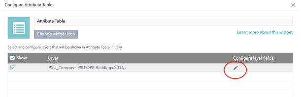 Figure 1.16 Configuring the Attribute Table widget in Web AppBuilder
Now let's modify the widgets that are held within your theme's widget container (or controller).
- Regardless of the theme you selected, you should see a Set the widgets in this controller link near the top of the tab. Click on this link. You should see the Legend and Layers List widgets by default.
For this simple map in which the title makes it clear what's being shown, a legend is unnecessary.
- Hover your mouse over the Legend widget and click on the X in the upper right to remove it from the app.
For the same reason, you could probably also remove the Layer List widget. However, this widget provides a context menu of options that could be of interest to users.
- Hover your mouse over the Layer List widget and click on the pencil icon to change its configuration.
- Uncheck the Show Legend box. The widget makes it possible to view a legend for each layer by clicking on a small arrow to the left of the layer name, but again, there's not much point in a legend here.
The widget also offers the ability to perform certain actions through the context menu. All of these items are turned on by default, but you can override that.
- Uncheck the Enable/Disable Pop-up box and the Move up/Move down box (with only one layer on the map, the Move options will be disabled anyway).
- Click OK to dismiss the Layer List dialog, then Save your app.
- Click the Launch button to open your app in a new tab and confirm that the various settings you've made have taken effect.
Now let's check out some of the other in-panel widgets that are available.
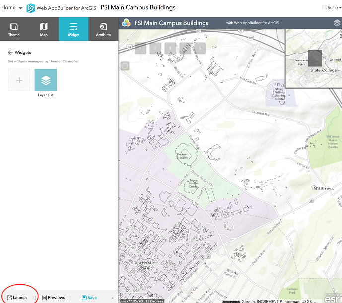 Figure 1.17 Launching an app preview in Web AppBuilder
- Close the tab containing your running app and return to the Web AppBuilder tab.
- Under the Widgets heading, click on the + sign to add a new widget. In addition to the Layer List and Legend widgets that we've already seen, you should see many others including Basemap Gallery, Edit, and Geoprocessing, among others. Being able to switch basemaps is a nice feature to have, even in a very simple demo like this, so let's provide that capability.
- Click on the Basemap Gallery widget and click OK. You'll be taken immediately to a configuration panel, which for this widget provides the ability to use your organization's basemap gallery (which will be the same as Esri's if your organization hasn't defined one) or configure a custom gallery for this app.
- Choose the Configure custom basemaps option, then click the Import button.
The Import basemaps dialog allows you to pick and choose from the full set of basemaps found in Esri's or your organization's gallery. Esri's gallery is selected by default.
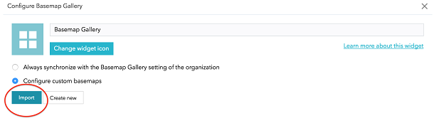 Figure 1.18 Customizing the basemap option in Web AppBuilder
- Click on each of the basemaps one at a time to add them to this app's gallery, with the exception of Imagery with Labels (it differs little from Imagery in this area), Oceans (not applicable to this area) and Terrain with Labels (not intended for use at this scale). Click OK twice to finish configuration of the Basemap Gallery widget.
- Click again on the + sign, add the Draw widget, check the box to Add the drawing as an operational layer of the map and click OK. This will enable the user to add custom features and annotation as a separate layer.
Now let's say you want the widgets to appear in a different order.
- Click on one of the widgets and drag it to a new position. You should see a red vertical line indicating where the widget will end up when you release the mouse button.
Before leaving the Widgets tab, there are a few more points worth mentioning:
- The Analysis widget provides access to several analytical tools that may be useful depending on the app's purpose (e.g., Create Buffers, Create Viewshed, etc.). Keep in mind though that usage of these tools may consume service credits allocated to your ArcGIS Online organization.
- The Edit widget can be used to develop online editing apps.
- The Geoprocessing widget can be used to "wire up" your app to a geoprocessing task.
- Full documentation for all of Esri's widgets can be found at Web AppBuilder for ArcGIS.
- Click on the Attribute tab to move on to a set of options that help with branding your app.
- Enter a sensible Title, such as Penn State University Park Buildings.
- If you're not interested in advertising for Esri, clear the text in the Subtitle box or assign your own.
- Set the app's logo (using the same Nittany Lion shield from the previous page) by hovering over the Logo icon, clicking the Custom link and browsing to the image on your computer. Note that the logo is not displayed for all themes.
- Click on Add New Link, enter www.psu.edu in the first box (the text that you want to display) and the URL http://www.psu.edu in the second box. Again, note that links are not displayed for all themes.
- Finally, Save your app, then click Launch to see the app as an end user would.
1.2.3 Creating an App with the Experience Builder
1.2.3 Creating an App with the Experience Builder
As we saw with the Map Viewer and configurable app templates, there is also a newer technology for building apps from scratch -- Experience Builder. Let's walk through creating a similar app on that platform.
- Re-open your Buildings map using the current Map Viewer, click Create app, then Experience Builder.
You'll be presented with several templates to use as a starting point. Each one is shown in wireframe form to give you a quick preview of its widget layout. Note that you can hover over these wireframes to get a description of the template or click the Preview buttons to get a better idea of the template's layout. A number of templates could work here; let's go with Foldable. - Click the Create button associated with the Foldable template.
- Feel free to go through the short tour of how Experience Builder works, or click Skip.
Where Instant Apps are designed to get an app up and running quickly by walking through a short set of numbered steps, Experience Builder is much more open-ended and can appear overwhelming at first. But let's break down the most important aspects of the interface.
The largest panel, in the middle, shows your app in a sort of design view referred to as the canvas.
To the left of the canvas is the sidebar, a panel whose contents depends on which of the four tabs on the very left side of the window is selected. These tabs, working from top to bottom, allow you to add new widgets to the app, access the widgets already included in it, define the data used by the app, and set an app theme.
To the right of the canvas is a settings panel, which shows settings associated with whatever widget is selected either in the sidebar or the canvas. - If it's not already selected, select the Page tab.
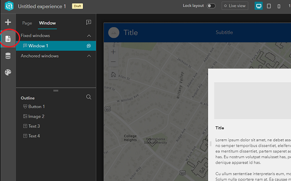
Figure 1.19 Selecting the Page tab in Experience Builder
On the canvas, you should note a "fixed window" -- having an ID of Window -- resembling a splash screen. - If the canvas is zoomed in on your app and you'd prefer to see all of its elements, you might like the Fit width to current window button, the second button in from the right side of the window, in the narrow strip of controls running along the bottom of the window.
"Window" contains placeholders for an image, two text elements (one for a title and one for the app description), and a button (to dismiss the window).
- Select Image 2, either in the sidebar or on the canvas. This will populate the settings panel to the right with the settings associated with that image.
- Working in the settings panel, modify Image 2 by going to Select an image > URL, and setting the URL to http://www.e-education.psu.edu/geog863/sites/www.e-education.psu.edu.geog863/files/PSU_UPO_RGB_2C.png.
- Double-click on the Title element (Text 3) on the canvas to edit that text and set it to Campus Buildings Map.
- Likewise, set the description (Text 4) to Enter a text string in the search box to find all buildings containing your search string.
We won't change anything else in the Window widget, but note that the checkbox text and button label are customizable. You might also choose to shrink the Window in size since the amount of text being displayed is small. - Finally, in the sidebar, hover your mouse over the Window entry. You should see a small "word balloon" icon that is identified as the Set as splash button. The Window widget should be set as a splash window by default, so you should not need to click this button. If you do, you'll be disabling the splash behavior. This isn't a very well designed setting as there doesn't appear to be any indicator for a window being set as splash or not...
- To access the map and other widgets in the background, click on the Page tab at the top of the sidebar. (The Window tab has been selected up to this point.) Again, the Fit width to current window button could come in handy here.
- Looking at the info in the sidebar, note that the app is composed of a single page, and that page contains a Sidebar widget (named Sidebar), not to be confused with the sidebar panel that is part of the larger Experience Builder interface. The Sidebar widget covers the entire canvas and is a container for other widgets. As its name implies, it can be used to display widgets in a primary panel and a secondary panel (on the side).
The widgets nested within "Sidebar" can be viewed by expanding the containers listed in the Experience Builder sidebar.
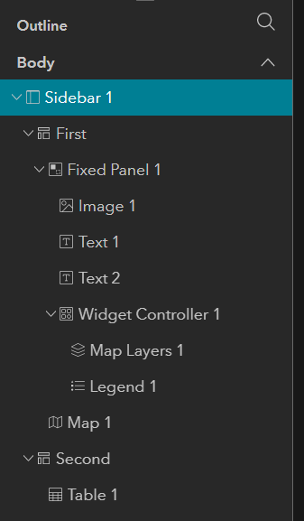
Figure 1.20 Contents of the Sidebar widget
The First (primary) container holds a Fixed Panel widget (the strip running across the top of the app) and a Map widget. The Second (collapsible side) container holds a Table widget. - Click on Sidebar in the sidebar and note in the settings panel that, among many other settings, it's possible to specify which side the Second container is docked on, the size of the Second container, and whether it is Collapsed or Expanded by default. Feel free to change any of these settings if you like.
As noted, the Second container holds a Table. Let's make sure that widget is configured properly. - Select Table in the sidebar to view its settings.
- Click New sheet > Select data, then expand the list of layers/tables in your PSU Buildings web map.
- Finally click on the buildings layer to select it as the source for Table's data. You should see the table become populated with data on the canvas.
As we did earlier, let's limit the fields shown in the table. - Click on the 7 selected dropdown, which will display each of the table's fields alongside a checkbox.
- Since we want to toggle off most of these fields, click the Clear Selection button in the lower right of the list.
- Toggle on the FID, BLDG_NAME_, and Shape_Area fields, then click again on the dropdown menu (which should now say 3 selected) to dismiss the field selection interface.
The rows showing in the table have no BLDG_NAME_ value, unfortunately. It would be nice if we could filter out unnamed buildings...
In the Sheet configuration panel, where the buildings layer is shown as the data source, there is a dropdown list with Default selected. The Default refers to the default view of the data. If the scenario called for it, we could define custom views of the data (say, those with a Shape_Area greater than a certain threshold), assign names to those views, and choose to have the widget show the data associated with one of the views. We don't need to do that, but let's look at configuring the Default view. - Click on the view dropdown. The Default view should appear with a small Settings button (gear icon) next to it.
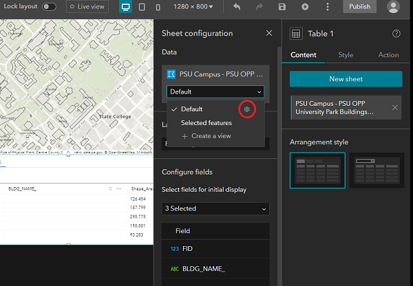
Figure 1.21 Accessing the Default view's settings
- Click on this Settings button.
The resulting dialog contains 3 tabs: Filter, Sort, and Records. Under the Filter tab, we could build a query that limits the rows returned to some subset, like just big buildings. Under the Sort tab, we can define sorting rules, and under the Records tab, we can control the number of rows that the table displays.
I encourage you to experiment with these capabilities. I attempted to display only rows where BLDG_NAME_ is not blank, but that didn't filter out the ones that have no name. I suspect those rows hold an empty string rather than a Null value, but had no luck with other attempts to filter them out. If anyone figures out how to solve this problem, please post how you did it in the Discussion Forum.
I also attempted to apply a useful sorting to the data. Sorting on BLDG_NAME_ isn't particularly useful as the empty rows still show up at the top of the list. And when I tried sorting in descending order on Shape_Area (putting the biggest buildings at the top), the data sorted properly in the dialog's preview, but not in the canvas. It appears that this is a known bug.
With the table configured, let's shift our focus to the strip of widgets found along the top of the app. - Click on Image (nested within Fixed Panel) in the sidebar.
- Set this image to display the PSU shield we used earlier in the lesson. Here's the URL again:
https://www.e-education.psu.edu/geog863/sites/www.e-education.psu.edu.ge... - And let's make this image a link that opens the Penn State home page:
Set link > Link to URL > https://www.psu.edu > Open in new window - Set the Title widget (named Text) to Penn State Campus Buildings and the Subtitle (named Text 2) to University Park. You may need to widen the Text element and shift the Text 2 element a bit to the right to get the text to show up properly.
As in our earlier apps, the Legend and Layer List widgets aren't really needed here. They could be removed individually by hovering over them in the canvas and clicking the X that appears in their upper-right corner or via the 3 dots menu in the sidebar. Or... - Since we don't need any widgets here, click on the 3 dots menu next to Widget Controller in the sidebar, then Delete to remove that complete set of widgets from the app. When asked whether you really want to do that, click Delete again.
The primary functionality that we want to build into this app is the ability to find a building by name. You may notice that there's already a Search icon in the upper right of the map, which seems promising. Let's see if we can configure that tool. - Select the Map widget in the sidebar. In the settings panel, note that we could choose to use a different web map or web scene as the source for this widget.
Scrolling down through the settings, note the Tools section, where we can see that the Zoom and Home tools are toggled on. Many other tools are available as well. However, there doesn't appear to be a way to customize the Search tool. Let's test out the app to see how that tool works. - First, give the app a more descriptive name by clicking on the Untitled experience 1 text in the upper left of the window and entering a new name like Penn State Main Campus Building Finder (Exp Builder).
- Next, click the Save button in the upper right to save the work you've done.
- Now, click the Preview button (the "Play" icon just to the right of Save) to open your app for testing in a new tab.
You should see "Window" appear in the foreground as a splash screen. (If you don't, you'll need to go back to Experience Builder, to the Window tab, then click the Set as splash button for the Window widget.) And you should be able to access the table by clicking the small arrow in the bottom middle of the app. - Open the Search tool and enter a test search term (e.g., Walker, for Walker Building, home of the Geography Department on the west side of campus). Depending on your search term, you may get a hit on a campus building, but you'll also get back matches on streets, towns, etc. It appears that the Search tool built into the Map widget is hardwired to use the ArcGIS World Geocoding Service.
How will we provide a way to search for matches in the buildings layer then? Well, we can configure the Map widget's built-in Search tool as we did earlier for the Instant App. - Return to the Experience Builder tab in your browser and expand the widget list within the Map in the sidebar. You should see an entry for the Search widget you just tested.
- Click on the Search widget to open its properties.
- Click on the New search source button and go through the same steps you followed earlier so that the widget is configured to search the BLDG_NAME_ field in the buildings layer.
- Save your work and confirm that the app now allows for searching the building layer.
With that, you've built a few apps that could be implemented in real-world scenarios using both newer and older Esri technologies. Best of all, you didn't have to write a line of code. One thing I hope you'll take away from this exercise is to remember that these no-coding tools exist and to look for opportunities to take advantage of them.
Move on to the next page of the lesson to solidify what you've learned here with an assignment that requires you to build another app using data and requirements of your own choosing.
Assignment: Build an App of Your Own
Assignment: Build an App of Your Own
This lesson's graded assignment is in two parts. Here are some instructions for completing the assignment.
Part I
First, I'd like you to build a web mapping app with Esri technology (using either a configurable template, Instant App, the Web AppBuilder, or the Experience Builder). You are welcome to select the app's subject matter (perhaps something from your work) and the functionality it provides. If you're unsure of what to map, you might try searching ArcGIS Online, where there is a wealth of data.
Details matter! Make sure your app looks professional by modifying anything that looks unfinished. Text a user sees, whether in a widget, popup, or elsewhere should be human-readable (or have good aliases) and not look like a default or coded name. Also choose appropriate symbology and consider hiding unneeded fields.
You will have another opportunity to select your own final project at the end of the term. Keep that in mind when selecting data and/or functionality to incorporate into this project.
Part II
There are other web mapping platforms that offer features similar to ArcGIS Online (e.g., CARTO, MapBox, SimpleMappr, MangoMap, MapHub, and MapLine). For the second part of this week's assignment, I'd like you to experiment with one of these platforms, then share your thoughts on it in a recorded video. Here are some detailed instructions:
- Please go to the Assignment 1 Platform Review Sign-up page in the Lesson 1 module in Canvas to sign up for a platform. The sign-ups will be set up such that each platform will be covered by roughly the same number of students. (If there's another platform that you'd like to evaluate, check with the instructor first.)
- Limit your video to 5 minutes.
- In your video, be sure to discuss the following points:
- Cost
- Ease of use
- Data formats supported
- How it compares to ArcGIS Online (similarities, differences, things you like better)
- Can you build an app or just a map? (I.e., Is it possible to add functionality similar to Esri's Web AppBuilder widgets?) - What I'm looking for in this video is for you to talk through a demo of the platform. You may choose to summarize your major points through slides, though that's not required. You are not expected to have any face time in the video,
 though you certainly can if you like. There is a short tutorial on recording videos with ScreenPal in the course orientation, though you're welcome to record your video with some other software.
Deliverables
This project is one week in length. Please refer to the Canvas course Calendar for the due date.
- Post a link to your Esri app to the Lesson 1 Discussion Forum. (40 of 100 points)
- Post a link to your video review of a non-Esri web mapping platform to the Lesson 1 Discussion Forum (and/or Media Gallery in Canvas). This could be in the same or a different post as #1 above. (40 of 100 points)
- As part of your discussion forum post, include some reflection on what you learned from the lesson, how you might apply what you learned to your job, and/or concepts that you found to be confusing (minimum 200 words). (20 of 100 points)
- Complete the Lesson 1 quiz.
Summary and Final Tasks
Summary and Final Tasks
With that, you've finished working through the content on developing geospatial apps without programming. For some of you, especially those who work in an organization with an ArcGIS Online account, what you've learned in this lesson will sufficiently meet your app development needs. However, if you find that the available widgets can't quite be added together to form the app you want, you'll need to learn about web programming technologies. In the next lesson, you'll learn about HTML and CSS, languages that are used to define the content and presentation style of web pages. With that foundation laid, you'll be ready to spend the rest of the course learning about Esri's JavaScript-based Application Programming Interface (API), which provides developers a finer level of control over their apps than is possible with their non-programming options.
IMPORTANT: Beginning in Lesson 2, you'll be expected to post some of your assignments to a web server. If you haven't already done so, please have a look at the page on e-Portfolios. In particular, the application for web space from PSU can take a business day or two, so you should get this taken care of in advance of having to post your Lesson 2 assignment.
Lesson 2: Creating a Field Data Collection App
Overview
Overview
In this lesson, we’ll walk through the configuration of a web map that can be viewed using Esri's Field Maps mobile app and used to record observations made in the field. This will give you exposure to another app development framework, one that has a specifically mobile device focus.
We'll actually be replicating work done recently by a Penn State MGIS student for his capstone experience. To set the stage for what we'll be doing, let's begin with a bit of background.
The Pennsylvania Department of Conservation of Natural Resources (DCNR) is the state agency charged with maintaining the state’s parks. One of their maintenance tasks is the remediation of invasive plant species. Unfortunately, limited funding makes it impossible to conduct remediation in all of the park locations where invasives are observed. For this reason, DCNR worked together with a Penn State College of Agricultural Sciences researcher to devise a methodology for prioritizing which of the infestations should receive the agency’s attention.
Within each park of interest, DCNR staff first delineate areas of similar ecological characteristics (habitat management zones, or HMZs). Each HMZ is assigned to one of 7 habitat types: Mature Forest, Pole Forest, Young Forest, Wetland, Riparian Corridor, Lakeshore, and Herbaceous Opening.
In developing an invasive species management plan (ISMP), priority scores ranging from 0-9 (?) are derived based on the following factors:
- Stewardship value – What is the HMZ’s value from an ecological stewardship standpoint?
2 = highest ecological value
1 = medium ecological value
0 = lowest ecological value - Outreach value – How much interest does this HMZ generate with outside groups (as a funding or volunteer source)?
2 = highest interest
1 = medium interest
0 = lowest interest - Extent value – How large is the species infestation?
2 = not present or in very low numbers
1 = medium presence level
0 = large infestation - Impact value – How severely does the species affect the HMZ’s native plant community?
1 = Super Bad
0 = Regular Bad
The impact a species has on the various habitat types is a known relationship that can be looked up as needed. For example, the Japanese knotweed has an impact value of 1 in an HMZ of the Lakeshore type, but 0 in the Forest types. - Restoration effort value – What level of effort will be required to eliminate the invasive?
3 = lowest effort; native plants fill in on their own after invasive is suppressed
2 = at least two seasons of suppression required
1 = elimination of invasive possible, but likely requires seeding/planting native plants
0 = highest effort; complete elimination of invasive unlikely
These values are also known ahead of time and vary based on the species and its extent value. For example, the Norway maple has a restoration score of 1 when its extent is rated as 0 (large infestation), a score of 2 when its extent is rated as 1, and a score of 3 when its extent is rated as 2 (in low numbers).
The priority score is calculated as follows:
priority = stewardship + outreach + extent + impact + restoration
The original form of this ISMP was an Excel workbook in which staff entered HMZ info and species observations into multiple tabs. VBA macros automated the priority score calculations. Unfortunately, this system had no spatial component.
More recently, a Penn State MGIS student devised a version of the ISMP for ArcGIS Field Maps. Through this application, DCNR staff can conduct their work in a spatial context by clicking/tapping an HMZ of interest on the map, recording the species found within it, and automatically obtaining a remediation priority score.
Objectives
At the successful completion of this lesson, students should be able to:
- build their own online/mobile map using Field Maps
- have a better understanding of the various map development / deployment frameworks available
- be able to choose an appropriate map framework for a particular task
- use Esri's Arcade scripting language to populate form fields automatically
Questions?
If you have any questions now or at any point during this week, please feel free to post them to the Lesson 2 Discussion Forum.
Checklist
Checklist
Lesson 2 is one week in length. (See the Calendar in Canvas for specific due dates.) To finish this lesson, you must complete the activities listed below. You may find it useful to print this page out first so that you can follow along with the directions.
| Step | Activity | Access/Directions |
|---|---|---|
| 1 | Download the Lesson 2 file geodatabase | Download here |
| 2 | Download Esri's Field Maps app to a phone or tablet (compatible with Android or iOS) |
Search for Field Maps on Google Play or Apple's App Store |
| 3 | Work through Lesson 2. | Lesson 2 |
| 4 | Take the Lesson 2 Quiz after you read the course content. | Click on "Lesson 2 Quiz" to begin the quiz. |
2.1 Publishing the web layer
2.1 Publishing the web layer
Take a few moments to explore the feature classes, tables, and domains in the ismp file geodatabase that you downloaded in ArcGIS Pro. The HMZ feature class contains 14 habitat management zone polygons covering Nescopeck State Park. Note that the HMZs are assigned an integer ID and a name. The feature class also contains empty fields for the stewardship and outreach indices discussed earlier.
The Species table contains the common and scientific names of the invasive plant species that may be found in the state.
The Species_HMZ table is where observations of invasive species within a HMZ can be recorded (via the Common_Name and HMZ_ID fields). Also in this table are fields for recording the various ratings discussed earlier: the extent of the invasive, its impact rating, its restoration rating, and finally, its cleanup priority score.
The last two tables – Impact and Restoration – are lookup tables that allow for determining the impact rating of a species given the habitat type it’s found in and the restoration effort rating of a species given its extent.
Lastly, the geodatabase contains several domains, which we’ll use to place limits on what can be entered in the various fields we’ve discussed (and to provide dropdown lists of options).
-
Apply the HabitatTypes domain to the Type field in the HMZ feature class (right-click on HMZ, Data Design > Fields, then choose HabitatTypes under Domain for the Type field). Likewise, apply the StewardshipVals domain to the Stewardship field and the OutreachVals domain to the Outreach field.
-
Next, similarly open the field design dialog for the Species_HMZ table and apply domains to the fields as follows:
SpeciesNames to Common_Name
ExtentVals to Extent_Value
ImpactVals to Impact_Value
RestorationVals to Restoration_Value
Our goal for this app is for the end user to be able to tap on a HMZ polygon, record a 0-2 stewardship rating and a 0-2 outreach rating for that HMZ, then record any number of invasive species observed in that HMZ (including the various other ratings found in the Species_HMZ table). One requirement imposed by Field Maps is that each layer/table you’d like to edit must contain a GlobalID field. This is a field, managed by ArcGIS, that stores a globally unique identifier, or GUID (https://www.techtarget.com/searchwindowsserver/definition/GUID-global-unique-identifier#:~:text=A%20GUID%20(globally%20unique%20identifier,accounts%2C%20documents%20and%20other%20items.), for each feature/row. -
Right-click on the HMZ feature class in the Catalog pane and select Manage. This will open the Manage tab of the Feature Class Properties dialog. Check the Global IDs checkbox and click OK to add a GlobalID field to the feature class.
-
Since we also want to be able to edit the Species_HMZ table, carry out the same action for that table.We're going to skip this step - I've struck it out because it's very likely to be unnecessary.Another important step in preparing our database will be to create a relationship class between the HMZ feature class and the Species_HMZ table. As part of this step, we’ll be specifying the primary key field for the HMZ feature class. This will be the GlobalID field we just added to that feature class. We’ll also need to specify the field in the Species_HMZ table that should be used to maintain the HMZ-Species_HMZ relationship (i.e., to link each Species_HMZ record to the correct HMZ).
-
Go into the Species_HMZ table’s field design dialog and add a new field with these parameters:
Name: HMZ_GUID
Alias: HMZ_GUID
Data Type: GuidBoth GlobalID fields and Guid fields store GUID values. The difference is that GlobalID fields are automatically managed by ArcGIS, whereas Guid fields are not. The purpose of this field we’re adding here is, as was just mentioned, to act as the linkage between the rows in the Species_HMZ table and the associated features in the HMZ feature class.
-
Create the relationship class by right-clicking on your geodatabase and selecting New > Relationship Class. In the Create Relationship Class tool dialog, make the following settings:
Origin Table: HMZ
Destination Table: Species_HMZ
Output Relationship Class: HMZ_Species_HMZ_RC
Cardinality: One to many
Origin Primary Key: GlobalID
Origin Foreign Key: HMZ_GUID
Leave all other options set to their defaults, then click Run to create the relationship class. -
If you haven’t already, add the HMZ feature class to a new map. Also add the 4 tables: Impact, Restoration, Species, and Species_HMZ.
-
Change the display of the HMZ layer so that it uses a Unique Values symbology based on the Type field (or the HMZ_ID field, your choice). (I’m partial to the Cool Tones color scheme myself.)
We’re now ready to publish the contents of the map to ArcGIS Online (AGO) so that it can be used in a Field Maps app. -
Go to Share > Web Layer > Publish Web Layer.
-
In the Share As Web Layer tool dialog, make the following settings under the General tab:
Name: ISMP Web Layer <your username>
Folder: Create a new folder called fieldmaps
Accept the defaults for all other options on this tab, but do not publish yet. The reason we're calling our layer something like "ISMP Web Layer aaa123" is that all of our layers need to have a unique name in AGO. -
Under the Configuration tab, click the pencil icon next to the Feature layer to access a number of configuration options. Check the Enable editing checkbox, leaving all of the edit types checked and the Attributes and geometry option selected.
-
Click Analyze to run a check of whether the map can be successfully published.
You should get 2 warnings of “Layer’s data source is not supported.” This is in reference to the two background layers that are included in ArcGIS Pro maps by default. It’s not strictly necessary, but remove these layers from the map.
The other issue you’ll see noted in the Analyzer results is an error that “Unique numeric IDs are not assigned.” Let’s take a moment to reflect on what we’re doing here. We’re hoping to make all the items loaded in the map -- the polygon layer and standalone tables – available for use in AGO. The singular name of “web layer” may seem confusing since our map could have any number of layers/tables in it, but that is the term for what is being produced in AGO. Each layer/table found in this Pro map is going to be published to AGO. One of the requirements before we can publish is that each layer/table needs a unique ID assigned to it. This can be done through a Map Properties setting, which we can access via a shortcut in the Analyzer results.
-
In the Analyzer results, hover your mouse over the error, click the … button, then select Open Map Properties to Allow Assignment.
-
Under the General settings, put a check in the Allow assignment of unique numeric IDs… checkbox, then click OK to dismiss the Map Properties dialog.
You should see the red X in the Analyzer results change to a green checkmark.
-
Click Analyze again. You should now receive no errors or warnings.
-
Click Publish. The Share As Web Layer tool will churn for a minute or two, before you should see a message that the web layer published successfully.
You should now be able to browse to your AGO account and see a hosted feature layer and service definition both with the name ISMP Web Layer.
Field Maps operates on web maps, so before we can create an app with Field Maps we’ll first need to create a web map containing our new web/feature layer.
-
While looking at the items in your fieldmaps AGO folder, click the … next to the feature layer and select Open in Map Viewer.
-
At this point, we could modify the layer’s symbology or how info is displayed in its popups. However, let's hold off on doing any such configuration for now. Simply click the Save and open button, assign a name of ISMP Web Map, specify that you want to put it in the fieldmaps folder, then click Save.
-
Return to your AGO Content page ("hamburger" icon in the upper left > Content), where you should now see the newly created web map. Click the … next to it and select Open in Field Maps Designer.
Note: I attempted two variations on this workflow, but neither was successful:
- Using the Share as Web Map tool in Pro instead of Share as Web Layer. This both creates the new AGO feature layer and a web map containing that layer, cutting out the need to add the new feature layer to the Map Viewer and save a web map as separate steps. However, feature edits in a web map created in this way didn't work for me as required.
- Creating the relationship class as many-to-many rather than 1-to-many. Each HMZ can have many species and each species can appear in many HMZs. Creating the relationship class in this way would automatically create an intermediate table that would store the HMZ-species combinations. However, again, feature edits didn't work as required when I attempted to go this route.
With the necessary data published to AGO and a web map created from it, we're now ready to configure the web map for staff who will be opening it in the Field Maps app on their mobile devices.
2.2 Configuring forms in Field Maps
2.2 Configuring forms in Field Maps
The primary type of configuration that is required in building a Field Maps app is creating forms for the end user to record their observations.
-
Click on the Forms button. You should see the HMZ layer under the Layers heading. And if you expand the Tables, you should see the map’s four tables, with only Species HMZ being enabled for form creation. (Note: Field Maps removes underscores from layer/table names, for whatever reason, so your table will show up as Species HMZ rather than Species_HMZ.)
-
Re-expand the Layers listing and click on HMZ to select it. You should see a design canvas appear in the middle of the window delineated by a box with a dashed outline. To the right of the design canvas, you’ll see a Form builder panel containing several different types of Form elements (or controls). Scrolling down through the Form builder controls, you should see the layer’s Fields at the bottom. One option for configuring a form is to drag and drop controls from the Form builder panel onto the design canvas. However, what we’ll do here instead is ask Field Maps to create a form from the layer’s popup.
-
Click the blue Convert pop-up button in the middle of the design canvas. You should see fields from the HMZ attribute table have been added to the canvas as text boxes (for fields without an associated domain) and as combo boxes (for fields with an associated domain).
-
Click the Save button in the upper right of the design canvas to save the form.
-
Expand the Tables listing and go through the same process to create a form for the Species_HMZ table.
You may not realize it, but you now have an app that you can test!
-
Open Field Maps on your mobile device. After logging in to your AGO account, you should be presented with a list of web maps.
-
Find your ISMP Web Map and tap it to open it.
Unless you happen to live in the vicinity of the Nescopeck State Park, you won’t be able to see the HMZ features. -
Open the Field Maps menu using the … button in the upper right and choose Bookmarks > Default Map Extent. This will zoom you to the park.
-
Tap the Campground Management Area (the square-ish polygon in the north-central part of the map) to select it.
You should see a popup appear showing the data associated with that HMZ. A DCNR employee using the app would want to record the Stewardship and Outreach ratings for the HMZ. -
To do that, tap the Edit button at the bottom of the screen (pencil icon). You’ll have the ability to modify the HMZ’s boundary, though there is no need to do so.
-
Instead, drag the popup panel up so that you're able to focus on attribute entry, then tap on the Stewardship box and choose 2 - highest eco value from the options (which came from the domain you configured).
-
Then tap on the Outreach box and choose 0 - lowest interest from the options. Click Submit to commit your entries to the geodatabase.
The DCNR staffer would next want to record the invasive species observed in the HMZ. With the popup panel up, scroll down past the HMZ attributes. You should see a Related heading followed by a Species HMZ link. -
Tap that link to access the related records from the Species_HMZ table. There aren’t any records as of yet, but you should see an Add button, enabling you to enter a new record.
-
Upon tapping Add, you should see a form containing the Species_HMZ fields. The HMZ_ID field will hold 0. You can either change that to the appropriate value (12) or just ignore it for now. We’ll come back to this in the next section. Make the following entries in the form:
Common_Name: exotic biennials
Extent_Value: 2
Impact_Value: 0
Restoration_Value: 2
Priority: 6
Note that the HMZ_GUID value will be automatically populated with the Campground Management Area’s GlobalID value, which happens because of the foreign key setting we made when configuring the relationship class. -
Tap Submit to commit this data to the Species_HMZ table as a new record.
With that, you will hopefully have successfully tested your app!
2.3 Populating fields automatically with calculated expressions
2.3 Populating fields automatically with calculated expressions
As you were testing, you probably saw some aspects of the app that could be improved. We already noted that the HMZ_ID of a new Species_HMZ record defaulted to 0 and in this section we'll correct this shortcoming by configuring a calculated expression written in Esri's Arcade scripting language.
Also, returning to the project background, you may recall that the Impact rating is based on the HMZ’s habitat type. Similarly, the Restoration rating is based on the species and its extent. So after the relatively simple HMZ_ID expression, we'll up the ante a bit to create more complex expressions that populate the Impact_Value and Restoration_Value fields by querying the Impact and Restoration lookup tables. We’ll also then be able to carry out the Priority score calculation using the various ratings entered by the user and derived from the lookup tables.
2.3.1 Getting the HMZ_ID
2.3.1 Getting the HMZ_ID
Recall that maintaining the relationship between the HMZ polygon feature and the Species_HMZ records associated with it depends on the GlobalID of the HMZ being entered into the Species_HMZ table’s HMZ_GUID field. That was a result of the relationship class we created. While this does maintain the record associations, the HMZ_GUID value (randomly generated by ArcGIS) will have no meaning to someone who views the Species_HMZ records in isolation. That's what drove the inclusion of HMZ_ID in the Species_HMZ table; it’s an ID assigned by the DCNR staff. However, as we saw, this field won’t be automatically populated for us. So let’s see how we can use Arcade scripting to populate this field.
-
In AGO, re-open your ISMP Web Map in the Field Maps Designer.
-
Return to the Form designer interface and re-open the Species HMZ table’s form.
-
Click on the HMZ_ID control to select it. You should see its Properties appear in the panel to the right.
-
Scrolling down that panel, you should see an area labeled Logic that has a Calculated expression property. Click the gear icon to access the calculated expressions stored with the web map. (There won't be any at this stage.)
-
Click New expression.
A dialog will open for building an Arcade expression, with a large box on the left for the expression and a collapsed panel on the right providing helpful shortcuts. The shortcuts are in the form of Profile variables and Functions.The profile variables provide a number of potential starting points for expression building. These include:
$feature – the feature whose attributes the user is currently viewing (or as in this case, a record from a standalone table rather than a feature from a feature class)
$map – the web map the user is currently viewing
$layer – the layer/table that the current feature/record is coming from
$featureSet – the complete set of features/records associated with the current layer; similar in concept to an array, common in programming languages; can be iterated over using a loop
$datastore – the complete set of layers/tables that are built into the web map
The Functions tab gives access to many general purpose functions found in many languages (e.g., Left, Right, Length, Count, etc.) along with spatial functions (Area, Centroid, Distance, Extent, etc.).
In order to retrieve the HMZ_ID value, we need to get at the HMZ feature associated with the currently open Species_HMZ record. We can do that by a) getting the HMZ_GUID, b) querying the HMZ layer for the HMZ feature with that value in its GlobalID field, and c) asking for the value in that feature’s HMZ_ID field. -
Start with step a) by entering the following:
var hmz_guid = $feature["HMZ_GUID"]
Note that:
- The var keyword is used in Arcade to define variables.
- Field values are accessed from features/records by quoting the field name and putting it in brackets.
- You can expand the $feature profile variable to the right to see a list of the fields available and to insert the field reference automatically (by clicking the appropriate link).Let’s confirm that we’re on the right track before moving on to the next step.
-
Add the following statement to the expression:
Console(hmz_guid)
-
Click the Run button in the upper left of the Expression box.
Field Maps may churn for a few seconds, but eventually you should see a new section appear in the interface beneath the Expression box. The Output tab will show the result returned by the expression – which we haven’t gotten to yet. What we want to look at now is the Console tab, which is where the Console function sends its output. Assuming all is well, you should see a GUID. (Recalling that $feature refers to the record currently being viewed, you may be wondering which record it’s referring to when testing here in the expression builder. I presume Field Maps is grabbing the first record it finds in the applicable table, Species_HMZ in this case.)
Returning to the expression, we can now work on step b) of the steps outlined above. Arcade has a FeatureSetByName function that can be used to get a reference to a FeatureSet (layer or table) through the global $map variable. -
First, remove the Console statement.
-
Next, get a reference to the HMZ layer, as follows:
var hmz_lyr = FeatureSetByName($map, "HMZ")
Please note that your layer might not be called just "HMZ" it's likely called "ISMP Web Layer aaa123 - HMZ" so you'll need to amend your code accordingly. To find out what your layer is called open it in Map Viewer and use the name in the Layers list.
Now we want to query the HMZ layer for all features where the GlobalID is equal to the value in our hmz_guid variable. -
Carry out this operation using the Filter function:
var qry = "GlobalID = '" + hmz_guid + "'"
var feat_set = Filter(hmz_lyr, qry)
Here we’re passing the Filter function a reference to the HMZ layer and a query expression. Note that GUID values must be quoted, so in creating the qry variable, the concatenation operator (+) is used to enclose the GUID in single quotes. When querying a layer in this way, the Filter function will return a FeatureSet object, which we’re storing here in the feat_set variable.
In other contexts, we might use a for loop to iterate over the Features in a FeatureSet. However, given the nature of GUIDs, we know that this FeatureSet will hold exactly 1 Feature.
-
Use the First function to get at the 1 returned Feature:
var feat = First(feat_set)
With a reference to the HMZ feature associated with the current Species_HMZ record, we’re ready to specify our Arcade expression’s return value (i.e., the value that should go into the HMZ_ID field). This is done in Arcade using the return keyword followed by the desired value.
-
Define the expression's return value, as follows:
return feat["HMZ_ID"]
Your complete Arcade expression should look like this:
var hmz_guid = $feature["HMZ_GUID"]
// remember that your layer might not be called "HMZ" so you
// might need to amend your layer name to be something like :
// ISMP Web Layer aaa123 - HMZ
var hmz_lyr = FeatureSetByName($map, "HMZ")
var qry = "GlobalID = '" + hmz_guid + "'"
var feat_set = Filter(hmz_lyr, qry)
var feat = First(feat_set)
return feat["HMZ_ID"]
-
With that, you can again click Run.
As the expression contains no Console statements, you should expect to see nothing under the Console tab. However, with the addition of a return statement, you should now expect to see something under the Output tab. Specifically, if you added a single Species_HMZ record associated with the Campground Management Area in your testing of the app at the end of the last section, you should see that the output returned by the expression is 12. -
Before leaving the expression builder, set the Title of the expression to getHMZ_ID.
-
Click Done to close the expression builder and return to the form designer.
Back in the form designer, you should now see a "Calculated" label beneath the HMZ_ID field and your getHMZ_ID expression listed under the Calculated value area of the Properties panel. -
Click the Save button in the upper right of the form designer to commit your changes.
-
At this point, you can return to Field Maps on your mobile device to test the change you just made. If you’re looking at the list of Maps available, you’ll probably see your ISMP Web Map listed under the Current heading. It’s probably a good idea to tap the … button next to it and then Reload Map to ensure the changes have made their way to your device.
-
Open the map and open the popup for the Campground Management Area again.
-
Access the related Species_HMZ form and click Add. The form associated with that table should appear and instead of defaulting to 0, the HMZ_ID should be set to 12. (It may take a second or two for the calculation to complete.) There’s no need to submit another species at this point, so you can tap Cancel and then Discard to back your way out of adding a new species.
That wasn’t a mission-critical calculation, but it did give a good introduction to writing calculated expressions with Arcade. You can learn more about the topic from the Field Maps documentation (https://doc.arcgis.com/en/field-maps/android/help/configure-the-form.htm...). In the next section, we'll build the expressions that are needed to compute the priority score for each Species_HMZ record.
2.3.2 Deriving the Impact and Restoration values
2.3.2 Deriving the Impact and Restoration values
Recall from the scenario that one of the ratings that contributes to a Species_HMZ record’s priority score is the Impact_Value ("regular bad" or "super bad"), which is dependent on which species is present and what type of habitat it’s invading (Mature Forest, Wetland, etc.). The application could be built with the expectation that the staffer would look up the impact value and enter it manually, but that lookup can be handled automatically with another calculated expression since we have the data needed in the Impact table. For example, looking in that table, we can see that the garlic mustard species in the Wetlands habitat type has an impact value of 1 (super bad).
Hopefully you’re already thinking through the steps that are required for this calculation. As in the previous one, we’ll want to obtain a reference to the associated HMZ feature. We can then get the value from the Type field. Another data point we’ll need is which species we’re dealing with. That we can access through the $feature variable. Having those two data points, we can query the Impact table to get the impact value associated with that species+habitat type combination. We’ll get to the Impact table through the $datastore variable.
One wrinkle involved in this query is that the Impact lookup table has been populated such that it contains only those species+habitat type combinations that have an impact value of 1 (the "super bad" ones). Thus, if a species+habitat type combination cannot be found in the table, it can be assumed that the impact value is 0 (i.e., that it’s a "regular bad" situation).
- Back in Field Maps, pull up the Species_HMZ form again.
- Click to select the Impact_Value field.
- Create a new Calculated expression for that field. (Note that the Calculated expressions area of the Properties panel will list all expressions you’ve written for this web map, not just for the field you currently have selected.)
- Copy and paste this expression (or type it manually, if you prefer):
var species = $feature["Common_Name"]
var hmz_guid = $feature["HMZ_GUID"]
// remember your layer might not be called "HMZ" but
// "ISMP Web Layer aaa123 - HMZ" so adjust it accordingly
var hmz_lyr = FeatureSetByName($map, "HMZ")
var hmz_qry = "GlobalID = '" + hmz_guid + "'"
var feat_set = Filter(hmz_lyr, hmz_qry)
var feat = First(feat_set)
var habitat_type = feat["Type"]

var impact_tbl = FeatureSetByName($datastore, "Impact")
var impact_qry = "Habitat_Type = '" + habitat_type +
    "' and Common_Name = '" + species + "'"
var impact_rows = Filter(impact_tbl, impact_qry)

if (Count(impact_rows) == 0) {
    //no match on this species+habitat, so impact is 0 (regular bad)
    return 0
} else {
    //there is a match on this species+habitat, let's get the impact value
    var impact_row = First(impact_rows)
    var impact_val = impact_row["Impact_Value"]
    return impact_val
}
Hopefully you’re able to follow everything going on in this expression. Here are a couple of points of clarification:
- Based on the design decision to omit records where the impact value is 0, note the use of the Count function to determine whether the query on the Impact table found any rows. The expression’s return value is set to 0 if a match is not found; otherwise, the return value is set to whatever is held in the Impact_Value field. (This field only holds values of 1, so alternatively the expression could just be set to return 1 when the query finds a match, but explicitly retrieving the value has the advantage of offering flexibility in the event that the impact rating scale were to change from something other than just 0-1.)
- The expression contains a couple of comments intended to clarify the logic involved. These are the lines that begin with double slashes (//). -
Assign a name to the expression of getImpact, then close out of the expression editor and Save your changes to the web map.
-
Return to the Field Maps app on your mobile device to test. (Remember to reload the map first.)
-
Again, select the Campground Management Area, and add a new species.
When the Species_HMZ form first opens, you should see the Impact_Value field automatically take on a 0 - regular bad value because the species name has not been specified yet. -
Choose a species found in the Impact table associated with the MF habitat type (wavyleaf basketgrass is one) and confirm that the Impact_Value field updates itself to 1 - super bad.
-
Cancel out of the edit once you’ve confirmed your expression is working as intended.
Recall from the scenario that the restoration effort rating is another field on the form that is derived from other user-supplied values. Specifically, it depends on the species in question and the extent of its infestation. Unlike the calculation of the impact value, which required obtaining one value from the Species_HMZ form and another from the HMZ form, the values needed for the restoration calculation are both found in the Species_HMZ form. So this expression will be a bit less complicated. -
Return to Field Maps in AGO and re-open the Species_HMZ form for editing.
-
Select the Restoration_Value field and open up the expression builder.
-
Take a crack at writing the expression yourself.
As noted above, you’ll need the user-entered species name and extent rating. You can then query the Restoration lookup table to get the restoration value associated with the species+extent combination. Like the Impact lookup table, combinations that yield a 0 value have been omitted from the table. Unlike it, however, the possible restoration values range from 0-3 rather than 0-1, so you would not have the option of assuming a value of 1 if a match for the species+extent combination is found.Code that completes the task can be found here:
var species = $feature["Common_Name"]
var ext = $feature["Extent_Value"]

var rest_tbl = FeatureSetByName($datastore, "Restoration")
var rest_qry = "Common_Name = '" + species +
    "' and Extent_Value = " + ext
var rest_rows = Filter(rest_tbl, rest_qry)

if (Count(rest_rows) == 0) {
    return 0
} else {
    var rest_row = First(rest_rows)
    var rest_val = rest_row["Restoration_Value"]
    return rest_val
}
We’ve now written expressions to automatically populate two of the important ratings fields, eliminating the need for a staffer to look them up manually. Recall that the ultimate purpose of populating those fields, and of the map itself, is to derive an overall remediation priority score. We’re now ready to build one last expression to carry out that calculation.
-
In the Field Maps form designer, select the Priority field and open up the expression builder.
Recall from the discussion earlier that the priority score is computed as the sum of the following five values:
Stewardship and Outreach (from the HMZ table)
Extent, Impact, and Restoration (from the Species_HMZ table). -
Using your expression building experience, see if you can come up with the code needed to populate the Priority field with the correct score.
Code that completes the task can be found here://Get the extent, impact, and restoration vals from the current Species_HMZ record var extent_val = $feature["Extent_Value"] var impact_val = $feature["Impact_Value"] var rest_val = $feature["Restoration_Value"] //Get the stewardship and outreach vals from the related HMZ record var hmz_guid = $feature["HMZ_GUID"] var hmz_lyr = FeatureSetByName($map, "HMZ") var feat_set = Filter(hmz_lyr, "GlobalID = '" + hmz_guid + "'") var feat = First(feat_set) var steward_val = feat["Stewardship"] var outreach_val = feat["Outreach"] //Sum and return the result var priority_val = steward_val + outreach_val + extent_val + impact_val + rest_val return priority_val -
Save the expression with a name of calcPriority.
-
Save your changes to the Species_HMZ form.
-
Return to the Field Maps app on your mobile device and go through the addition of a Species_HMZ row (woody vines, extent of 2, and butterfly bush, extent of 1, are other species found in the Campground Area). Confirm that both the Restoration_Value and Priority fields are populated automatically.
2.4 Applying finishing touches
2.4 Applying finishing touches
Tools like those built into Field Maps often set UI element properties to commonly used values in order to minimize the effort needed to produce a working app. However, just as a cartographer shouldn't leave .shp in the names of layers being shown in a legend, a developer should consider what changes can be made in default settings to produce a more professional and user-friendly UI.
If you haven't already, take a few moments to examine how the ISMP Web Map looks when open in Field Maps on your mobile device. Are there any fields being shown that would not be of interest to the end user? Are there any control labels that could be better tailored to the map's purpose or made more user friendly? Are the dropdown options presented in an intuitive order? On this page of the lesson we'll address the issues that I noted. If you think there are any other ways to improve the map, feel free to post your ideas to the discussion forum.
The first thing we'll do is look for fields in the HMZ form that aren't needed and only serve to clutter it. Looking at the map in the Field Maps app on your mobile device, the OBJECTID, GlobalID, Shape_Area, and Shape_Length fields offer little, if any, value, so let's get rid of them. But how? We have a few different options:
- Open the map in the AGO Field Maps form designer and remove the unneeded fields from the HMZ layer's form. This would cause the fields to no longer appear in Field Maps, but they would still appear in other contexts where the map is found.
- Open the map in the AGO Map Viewer and remove the unneeded fields from the HMZ layer's popup. This would cause the fields to no longer appear anywhere the map is found.
- Open the feature layer with the Map Viewer and remove the unneeded fields from the layer's popup. This would cause the fields to no longer appear everywhere the ISMP Web Map is used and in any other maps that include the layer.
All of a layer's fields are included in its popup by default. Interestingly, if you open the map with the Field Maps form designer, you'll see that the fields I mentioned (OBJECTID, etc.) do not appear on the form. Recall that we populated the form with controls by choosing to convert the layer's popup. The fields I mentioned aren't on the form and also aren't available to add. And yet, they do show up when the map is opened in the Field Maps mobile app. I don't know if this is an intentional design decision or a bug. In any case, to get these fields off the form, it means we'll need to modify the layer's popup.
- Open the ISMP Web Map in the AGO Map Viewer.
- The HMZ layer should be selected by default. Click the Pop-ups button found on the strip of buttons running along the right side of the map. A popup preview showing data from an example feature should appear over the map along with a panel of properties that can be set.
- Click on the Fields List button to expand the list.
- Click the X next to the OBJECTID field. You should see it disappear from the popup preview.
- Repeat for the GlobalID, Shape_Area, and Shape_Length fields.
- Close the Pop-ups panel.
The Save and open button running along the left of the Map Viewer (folder icon) should now have a blue dot over it, indicating that there are unsaved changes.
- Click that button, then Save.
There are likewise a few unneeded fields that appear on the Species HMZ form -- OBJECTID, GlobalID, and HMZ_GUID.
- Click the Tables button on the left side of the Map Viewer to access the tables included in the map.
- Select the Species HMZ table, then go through the same process used above to remove the three unneeded fields from the popup.
- Save your changes.
One thing you may not have noticed when configuring the forms in Field Maps is that the controls were all embedded within a Group layout element. On each form, this element was assigned a default label of Control 1. This label appears in the Field Maps mobile app, but interestingly, only for the Species HMZ form, not for the HMZ form. (The group label for the HMZ form is Fields, not Control 1, for whatever reason.) The mobile app user can tap this label to expand/collapse the field controls found within that group.
- Exit out of the Map Viewer and open the ISMP Web Map in Field Maps again.
- Open the Species HMZ form and select the Group control (the item on the design canvas with the label Control 1).
- In the Properties panel to the right, change the Display Name to Species-HMZ Attributes.
- Click the Save button in the upper right of the design canvas to commit your change.
One last improvement that we'll make concerns the selection of the species. The Common_Name dropdown list, which is populated based on the SpeciesNames domain you applied in Pro prior to publishing the web layer, is not in alphabetical order, making it quite tedious to find the desired species. There doesn't appear to be a convenient way in AGO to order the names. It can be done using the Python API for ArcGIS, but diving into that coding platform would be outside the scope of this class. Fortunately, there is a tool in Pro built for this purpose. And most importantly, making such a change won't require going through the entire workflow again. We can simply re-publish the web layer, choosing to overwrite it, and the change will be reflected in our web map (and any other web maps that happen to include the web layer).
- Return to ArcGIS Pro and open the geoprocessing toolbox (Analysis > Tools).
- Searching on the keyword sort, locate and open the Sort Coded Value Domain tool.
- Browse to your ismp geodatabase, selecting the SpeciesNames domain, and Run the tool so that the Code-Description pairs are sorted by Code in Ascending order.
- Re-publish the web layer by going to Share > Web Layer > Overwrite Web Layer.
- Looking within Portal > My Content, navigate into your fieldmaps folder and select your ISMP Web Layer.
A message will appear, warning that what you're about to do will cause you to lose changes that were made after the layer was initially published. This means losing the features/records that were added to the HMZ layer and the Species_HMZ table. This isn't really problematic as those were just test edits. Perhaps more consequential is the possibility of losing changes made in popup configuration. We just made changes of that kind, though recall that we made them by opening the ISMP Web Map in the Map Viewer rather than the ISMP Web Layer. That meant that we were taking the popup settings the web layer brought with it and overriding them within the current web map only. It also means that the changes we made should "survive" an overwrite of the web layer.
- You could click Cancel to back out of the overwrite now if you wanted, but go ahead and click OK.
- In the Overwrite Web Layer panel that appears, accept all of the default settings and click Publish.
- Go back to the Field Maps mobile app, reload the map, and test again. Confirm that the Common_Name dropdown list is now sorted and that the unwanted fields are not being shown. (You should expect any data edits you had made in earlier testing to have been lost.)
WIth that, we've finished our walkthrough of configuring a field data collection app. In the next section, you'll be prompted to take what you've learned and apply it to a different scenario.
Assignment: Configure a Field Maps Solution of Your Own
Assignment: Configure a Field Maps Solution of Your Own
If you're like me, every so often you bag up a bunch of old clothes to donate. But figuring out where to take them can be a challenge. Donation bin locations change fairly frequently and I've had limited success finding them through online searches. The scenario for this assignment is that you work for some organization -- perhaps a local government agency or a nonprofit -- interested in compiling the locations and other attributes of such donation sites in your local area.
Following a workflow similar to what you saw in the lesson, devise a Field Maps-based solution that can be used by staff working on tablets to compile the data. Here are some details on what is expected:
- You are welcome to expand this to include other household goods (e.g., electronics), but the basic requirement is to account for clothing and shoes.
- In addition to bins like the ones picture above, you should also build in support for capturing data on stores (e.g., Goodwill) and consignment shops. At minimum, this will require recording the name of the organization taking the donation, its hours of operation, and whether dropoffs can be made outside of those hours.
- This should be a less complex scenario than the invasive plant species one you just walked through, so don't overthink your solution.
- There is no need for complex Arcade expressions like those from the invasives scenario. However, I do want you to store the ID/name of the signed-in user and the date when an edit is performed. Guidance on how to do this, using Arcade, can be found in the documentation.
- Be sure to share your web map with the GEOG 863 AGO group for the current term so that your grader can access it!
Deliverables
This project is one week in length. Please refer to the Canvas course Calendar for the due date.
- Submit a document (Word or PDF) that contains the URL of your web map to the Assignment 2 Submission area in Canvas. (80 points)
- Include in the document some reflection on what you learned from the lesson and/or any concepts that you found to be confusing (minimum 200 words). (20 of 100 points)
- Complete the Lesson 2 quiz.
Lesson 3: Web Publishing Technologies: HTML/XHTML/CSS
Overview
Overview
A web mapping application is essentially a web page containing special scripts that dynamically add a map to the page. The bulk of this course will be concerned with writing these map building scripts (using JavaScript). However, web maps are embedded within pages written in the web publishing languages of HTML and CSS, so it makes sense to first spend some time discussing those languages.
This lesson covers a lot of material, so be sure to set aside enough time for it. At the end of the lesson, you'll be given a document and asked to apply what you've learned to produce a web page that replicates the formatting of your assigned document.
Objectives
At the successful completion of this lesson, students should be able to:
- understand the basic rules/terminology of Hypertext Transfer Markup Language (HTML);
- author a simple web page containing paragraphs, lists, tables, images, and links without the aid of an HTML editor;
- describe notation schemes that are not handled well by HTML;
- explain the need for and uses of eXtensible Markup Language (XML);
- describe the motivation behind the development of eXtensible HTML (XHTML) and its syntax differences from HTML;
- describe the benefits of using Cascading Style Sheet (CSS) technology;
- author a simple web page using XHTML and CSS.
Questions?
Conversation and comments in this course will take place within the course discussion forums. If you have any questions now or at any point during this week, please feel free to post them to the Lesson 3 Discussion Forum. (That forum can be accessed at any time by clicking on the Discussions tab.)
Checklist
Checklist
Lesson 3 is one week in length. (See the Calendar in Canvas for specific due dates.) To finish this lesson, you must complete the activities listed below. You may find it useful to print this page out first so that you can follow along with the directions.
| Step | Activity | Access/Directions |
|---|---|---|
| 1 | Work through Lesson 3. | Lesson 3 |
| 2 | The instructor will email you a Word Document. Reproduce that document as a web page using HTML and CSS. | Post your web page in your e-portfolio. |
| 3 | Take Quiz 3 after you read the online content. | Click on "Lesson 3 Quiz" to begin the quiz. |
3.1 HTML
3.1 HTML
HTML Basics
HyperText Markup Language (HTML) is the core language involved in the authoring of pages published on the World Wide Web. HTML is simply plain text in which the text is "marked up" to define various types of content, such as headings, paragraphs, links, images, lists, and tables. The markup occurs in the form of tags, special character strings that signal the beginning and end of a content element. For example, the <h1>...<h6> tags are used to define heading elements:
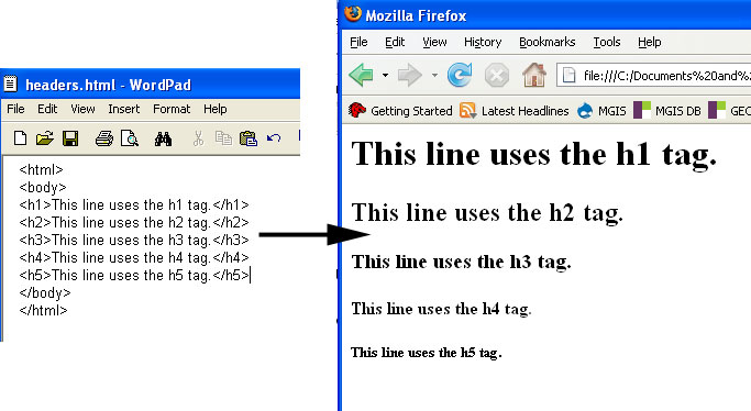
- The characters that denote an HTML tag (< and >) are referred to as angle brackets.
- Tags usually come in pairs (e.g., <body> and </body>, where <body> is the start tag and </body> is the end tag).
- HTML is not case sensitive (i.e., <title> is the same as <TITLE>), though lowercase is the recommended standard.
- Tags and their associated text form HTML elements.
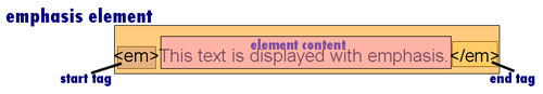
A simple HTML document
All HTML documents should be enclosed within <html></html> tags and should contain a head section and a body section. The head section contains metadata about the document and is defined using the <head> tag. The <title> tag is used frequently in the head section to define the title of the document. The body section contains the information you want to appear on the page itself and is defined using the <body> tag. Below is an example of a very basic HTML document:
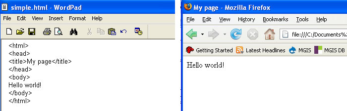
Commonly used tags
As we saw earlier, the <h1>...<h6> tags are used to define headings. Other tags that are often used to define elements in the body of a document include:
- <p></p> to define paragraphs of text
- <em></em> to give text emphasis (displayed in italics by default)
- <strong></strong> to give text strong emphasis (displayed in bold by default)
- <br> to insert a line break
- <hr> to insert a horizontal rule (line)
Note that a couple of these tags refer to the default presentation of their associated text. Later in the lesson, we'll see how stylesheets can be used to override these defaults.
Displaying lists
HTML allows authors to define two types of lists -- ordered and unordered. Ordered lists are most appropriate when listing a set of steps or items that can be ranked in some way. The <ol> tag is used to begin an ordered list and the </ol> tag is used to end it. Within those tags, each item should be enclosed within <li> and </li> tags. By default, web browsers number the items automatically beginning with 1.
| Code | Display |
|---|---|
<html>
<body>
<h4>Ordered List</h4>
<ol>
    <li>Citizen Kane</li>
    <li>Casablanca</li>
    <li>The Godfather</li>
</ol>
</body>
</html>
|
 |
Unordered lists are most appropriate when listing items that cannot be ranked meaningfully. List items are defined the same way with <li></li>, but the items are enclosed by <ul></ul> rather than <ol></ol>. By default, web browsers mark the items with bullets.
| Code | Display |
|---|---|
<html>
<body>
<h4>Unordered List</h4>
<ul>
    <li>Ford</li>
    <li>GM</li>
    <li>Chrysler</li>
</ul>
</body>
</html>
|
 |
Note: The indentation of the list items in the examples above is done merely to improve the readability of the HTML code and is not responsible for the indentation of the items in the output. Writing the code such that the li elements appear flush with the left margin would result in the same output.
Displaying images
Images are added to a web page using the <img> tag. For example:
<img src="brown_MarkerA.png">
Some important points to note about this example:
- img elements don't have an end tag.
- src is an example of an element attribute.
- Attribute values should be specified in quotes, preferably double quotes.
- The web browser will look for brown_MarkerA.png in the same folder that the HTML document is in.
- It is also possible to load images using a full web address (URL):
<img src="http:/detwilergeog863.webhostapp.com/icons/brown_MarkerA.png">
Adding links
Links are added to a web page using the anchor tag (<a>) and its href attribute:
<a href="http://www.psu.edu/">Penn State</a>
Note that the text that you want to display as a link should be placed between the <a> and </a> tags. The URL that you want to load should be used to specify the href attribute value.
You've probably encountered pages with links that jump to a specific location in the page (e.g., a "Back to top" link). This is called a bookmark link and creating one is a two-step process:
- Create an anchor somewhere in the document: <a id="top"></a>
- Link to that anchor: <a href="#top">Back to top</a>
Note that the value assigned to the id attribute ("top" in this case) is entirely up to you. The key is to plug the same value into the href attribute and precede that value with a pound sign to specify that you're linking to an anchor in the same document.
This will also work to link to a specific location in another page a bookmark link will also work to link to another page such as Lesson 3 Deliverables using:
<a href="www.e-education.psu.edu/geog863/node/1886#L2deliverables">Lesson 3 Deliverables</a>
HTML entities
Some of the characters you might want to display on your page require special coding because they have special meanings in HTML. For example, if you wanted to display an algebraic expression like x > 5, you'd need to use the code > since angle brackets are used to produce start and end tags.
Another aspect of HTML that can prompt the use of one of these entities is the fact that consecutive spaces in your HTML source code are treated as one. You can get around this by inserting one or more non-breaking spaces with the entity .
Some other commonly used entities include:
| Output char | HTML code |
|---|---|
| & | & |
| " | " |
| © | © |
| ÷ | ÷ |
| × | × |
HTML tables
Tables are commonly used in mapping applications to display information associated with features on the map. A table is defined using the <table> and </table> tags. A row can be added to the table using the <tr> and </tr> tags. Individual cells of data can be added to a row using the <td> and </td> tags. Here is a very simple example:
| Code | Display |
|---|---|
<table> <tr> <td>Penn State</td> <td>Nittany Lions</td> </tr> <tr> <td>Ohio State</td> <td>Buckeyes</td> </tr> </table> |
 |
To add a border to a table, you set its border attribute to some whole number (of pixels):
| Code | Display |
|---|---|
<table border="1"> <tr> <td>Penn State</td> <td>Nittany Lions</td> </tr> <tr> <td>Ohio State</td> <td>Buckeyes</td> </tr> </table> |
 |
To include column headings, add a row containing <th> elements instead of <td> elements. By default, web browsers will display the <th> elements in bold:
| Code | Display |
|---|---|
<table border="1"> <tr> <th>School</th> <th>Mascot</th> </tr> <tr> <td>Penn State</td> <td>Nittany Lions</td> </tr> <tr> <td>Ohio State</td> <td>Buckeyes</td> </tr> </table> |
 |
<td> and <th> elements have an attribute called colspan that can be used to spread the element's text across multiple columns:
| Code | Display |
|---|---|
<table border="1"> <tr> <th colspan="2">2000</th> <th colspan="2">2006</th> </tr> <tr> <th>Males</th> <th>Females</th> <th>Males</th> <th>Females</th> </tr> <tr> <td>5,929,663</td> <td>6,351,391</td> <td>6,043,132</td> <td>6,397,489</td> </tr> </table> |
 |
Likewise, <td> and <th> elements also have a rowspan attribute for spreading text across multiple rows.
Miscellaneous notes
Comments (text that you want to be visible when viewing the source code, but not in the rendered page) can be inserted into an HTML document using the following syntax:
<!-- This is a comment. -->
Also, as mentioned above, consecutive spaces are ignored by web browsers. This means that you should feel free to indent your HTML code (as shown in the table examples) and use line spacing to make it easier to read and follow.
Online tutorials/cheatsheets
This section of the lesson is just an introduction to the basics of HTML. There are many other helpful online HTML tutorials that can help you learn the language, along with cheatsheets that can be used for quick reference once you've gained some coding experience. Here is a list of sites that I've found to be helpful:
3.2 XML/XHTML
3.2 XML/XHTML
What is XML?
HTML handles the needs of most web authors, but there are some kinds of information that it is not well suited for presenting (e.g., mathematical notations, chemical formulae, musical scores). The eXtensible Markup Language (XML) was developed to address this shortcoming. XML is a language used to define other languages, a meta-language. Just as HTML has its own syntax rules, you can create your own markup language with its own set of rules.
For example, here is an example of a markup language used to store information about CDs in a CD catalog. Unlike HTML, in which the root element is called <html>, this language has a root element called <CATALOG>. A <CATALOG> element is composed of one or more <CD> elements. Each <CD> element in turn has a <TITLE>, <ARTIST>, <COUNTRY>, <COMPANY>, <PRICE>, and <YEAR>.
So, like HTML, XML documents use tags to define data elements. The difference is that you create the tag set. It is possible (though not required) to specify the rules of your XML language in a document type definition (DTD) file or an XML schema definition (XSD) file. For example, you might decide that a <CD> element can have one and only one <ARTIST> element within it.
While XML is quite similar in syntax to HTML (i.e., its use of tags), there are some syntax differences that make XML a bit more strict. Among these differences are:
- XML elements must have an end tag. Recall that the <img> element in HTML doesn't require an end tag.
- XML tags are case sensitive. <CATALOG> is not the same as <catalog> in XML, whereas <EM> is the same as <em> in HTML.
- XML elements must be nested properly. In HTML, an author can get away with code like <strong><em>Total</strong></em>, whereas in XML the </em> tag must come before the </strong> tag.
XML's Uses
XML has become an important format for the exchange of data across the Internet. And, as the CD catalog example discussed above implies, it can also be used as a means for storing data. We'll use XML later in the course for both of these purposes. Right now, we're going to focus on XML's use in creating a new flavor of HTML called XHTML.
An early development in the growth of web publishing was that desktop web browsers were designed to correct poorly written HTML. For example, in a bit of content containing paragraphs of text, it is possible to omit the </p> tag for paragraph elements and all of the popular desktop web browsers will render the content the same as if the </p> tags were present. This is not a surprising development if you think about it for a moment. Which browser would you prefer to use: one that displays a readable page the vast majority of the time or one that displays an error message when it encounters poorly written HTML?
Flash forward to the 2000s, the dawn of portable handheld devices like tablets and smartphones and wireless Internet. Slower data transfers and less computing power in these devices combined to produce lesser performance when rendering HTML content. This was one of the factors leading to the development of XHTML.
What is XHTML?
XHTML (eXtensible Hypertext Markup Language) is simply a version of HTML that follows the stricter syntax rules of XML. An XML/XHTML document that meets all of the syntax rules is said to be well-formed. Well-formed documents can be interpreted more quickly than documents containing syntax errors that must be corrected.
The introduction of this new XHTML language came after years of the development of plain HTML content. Thus, web authors interested in creating well-formed XHTML had to adjust their practices a bit, both because of the sloppy habits that forgiving browsers had enabled and the outright differences with HTML. These adjustments include:
- Elements that don't require an end tag in HTML must have one in XHTML (e.g., <p> needs a matching </p>).
- Empty elements in HTML must be terminated in XHTML (e.g., <br> must be changed to <br></br> or its shortcut <br />).
- Elements must be properly nested.
<strong><em>Some text</strong></em> INCORRECT
<strong><em>Some text</em></strong> CORRECT - Attribute values must be quoted.
<table rows=3> INCORRECT
<table rows="3"> CORRECT - XHTML is case sensitive. <a> and <A> are different tags. The standard is to use lowercase.
Flavors of XHTML
HTML was originally developed such that the actual informational content of a document was mixed with presentational settings. For example, the <i> tag was used to tell the browser to display bits of text in italics and the <b> tag was used to produce bold text. An important aspect in the development of web publishing has been its push for the separation of content from presentation. This resulted in the creation of an <em> tag to define emphasized text and a <strong> tag to define strongly emphasized text. It turns out that the default behavior of browsers is to display text tagged with <em> in italics and text tagged with <strong> in bold, which may leave you wondering what purpose these new tags serve if they only replicate the behavior of <i> and <b>.
The answer lies in the use of Cascading Style Sheets (CSS). With CSS, web authors can override the browsers' default settings to display elements differently. Authors can also develop multiple style sheets for the same content (e.g., one for desktop browsers, one intended for printing, etc.). The usage of style sheets also makes it much easier to make sweeping changes to the look of a series of related pages. We'll talk more about CSS in the next section.
So, while it is possible to override the behavior of the <i> and <b> tags just as easily as any other tags, the <em> and <strong> tags were added and recommended over <i> and <b> to encourage web authors to move away from the practice of mixing content with presentation.
XHTML has two main dialects that differ from one another in terms of whether they allow the use of some presentational elements or not. As its name implies, the XHTML Strict dialect does not allow the usage of elements like <font> and <center>. It also does not allow the usage of element attributes like align and bgcolor. Presentation details like font size/type and alignment must be handled using CSS. The Strict dialect also requires that all text and images be embedded within either a <p> element or a <div> element (used to define divisions or sections of a document).
The XHTML Transitional dialect does not prohibit the use of presentational elements and attributes like those described in the previous paragraph. Generally speaking, XHTML Transitional was intended for developers who want to convert their old pages to a newer version, but would probably not bother to do it if they had to eliminate every presentational setting. XHTML Strict was intended for developers creating new pages.
XHTML developers specify which set of rules their page follows by adding a DOCTYPE line to the top of the page. For example, here are the DOCTYPE statements for XHTML Strict and XHTML Transitional, respectively:
<!DOCTYPE html PUBLIC "-//W3C//DTD XHTML 1.0 Strict//EN"
"http://www.w3.org/TR/xhtml1/DTD/xhtml1-strict.dtd">
OR
<!DOCTYPE html PUBLIC "-//W3C//DTD XHTML 1.0 Transitional//EN"
"http://www.w3.org/TR/xhtml1/DTD/xhtml1-transitional.dtd">
Browse this article, Transitional vs. Strict Markup, for more details on the differences between the two dialects.
The basic skeleton of an XHTML Strict document looks like this:
<!DOCTYPE html PUBLIC "-//W3C//DTD XHTML 1.0 Strict//EN"
    "http://www.w3.org/TR/xhtml1/DTD/xhtml1-strict.dtd">

    <html xmlns="http://www.w3.org/1999/xhtml">
        <head>
            <meta http-equiv="content-type"
                content="text/html; charset=utf-8"/>
            <title>Your title here</title>
        </head>
        <body>
            Your content here
        </body>
    </html>
Page validation and conversion
XHTML and its dialects were developed by a standards organization called the World Wide Web Consortium (W3C). They also provide tools for web authors to validate that their pages follow the syntax rules of their selected DOCTYPE and to convert their pages from sloppy HTML to clean XHTML. This conversion tool is called HTML Tidy and can be run on the desktop or online (see links below).
Recent developments
Though XHTML was originally intended to be "the next step in the evolution of the Internet," it never gained a strong foothold in the web development community. A major factor that discouraged its adoption was that in order to reap the full benefit of an XML-based document, it needed to be served to browsers as "application/xhtml+xml" rather than "text/html." Most major browsers such as Firefox, Chrome, and Safari were built to handle the "application/xhtml+xml" content type. The notable exception was Internet Explorer, which until version 9 did not support "application/xhtml+xml" content — users were asked if they wanted to save the file when documents of that type were encountered.
In addition to the content type issue, technological advances have undercut the argument that small handheld devices cannot load web pages at an acceptable speed without the use of an XML-based parser. Today's smartphone browsers utilize the same HTML parsers as their desktop counterparts.
Thus, in recent years, the notion of a world in which browsers parse all web pages as XML and page developers must author well-formed documents appears less and less likely. The W3C halted their development of a new version of XHTML and shifted their focus towards a new version of HTML (HTML5). This led some to declare that "XHTML is dead." HTML5 requires browsers to continue correcting poorly written HTML. This has the effect of allowing sloppy page authors to continue in their sloppy habits. That said, browsers will continue to accept pages authored with XHTML-style coding, so developers who see value in serving their pages as XML may continue to do so. To learn more about HTML5, see the HTML 5 Introduction at the w3schools site.
So what language should we use?
HTML5 is the current standard for web publishing and you should certainly be looking to employ it in the web pages you develop. I have the content on XHTML in this lesson for a few reasons:
- to give you an appreciation for the evolution of web publishing standards,
- to encourage you to write clean HTML code. Doing so will enable you to achieve a higher level of consistency in the rendering of your pages than if you allowed yourself to pick up bad habits, and
- you may encounter XHTML in other people's source code.
At the end of this lesson, you'll be asked to write a web page from scratch using what you learned from the lesson. I'm going to require you to write that page in XHTML Strict. However, for subsequent projects, you will be able to use the less rigid HTML5.
3.3 CSS
3.3 CSS
The need for CSS
During the early years of the World Wide Web, maintaining a site where all of the pages share the same style was tedious and inefficient. For example, if a web author wanted to change the background color of each page on his/her site, that would involve performing the same edit to each page.
Creating alternate versions of the same page (e.g., one for the visually impaired) was also frustrating since it involved maintaining multiple copies of the same content. Any time the content required modification, the same edits would need to be made in multiple files.
Also, the mixing of page content with its presentational settings resulted in bloated pages. This was problematic for a couple of important reasons:
- It decreased the readability of the HTML source code, for example when performing edits.
- It increased the page's file size, which in turn increased the time required to download it.
The Cascading Style Sheet (CSS) language was developed to address all of these issues. By storing presentational settings in a separate file that can be applied to any desired page, it is much easier to give multiple related pages the same look, create multiple views of the same content, and reduce the bloating of pages.
How does CSS work?
To see how CSS works, go to this w3schools CSS demo. Click on a few of the "Stylesheet" links beneath the Same Page Different Stylesheets heading and note how the same exact content is displayed in a different way through the use of different style sheets.
Have a look at the page as rendered by "Stylesheet1," if you're not already, and view the page's source code (right-click on the page and select View Page Source) to see the CSS code stored in that style sheet. The beginning of this stylesheet tells the browser to display text within the document's body element at 100% of the size set by the user (as opposed to shrinking or enlarging it) and in the Lucida Sans font. It also applies a 20-pixel margin and a line-height of 26 pixels. Scrolling down to the bottom of the stylesheet, note that the a element is set to display in black (#000000) and with an underline. If you scan through the rest of the document, you should notice some other useful settings. Don't worry if you don't follow all of the settings at this point; you should have a clearer understanding after working through this page of the lesson.
The basic syntax used in CSS coding is:
selector {property: value}
where selector is some element, property is one of its attributes and value is the value that you want to assign to the attribute. I'll again refer you to the w3schools site for more CSS syntax and selector details. Pay particular attention to the "class selector," which is used when you don't want every element of a particular type to be styled in the same way (e.g., if you wanted some paragraphs to be aligned to the left and some to the right), and the "id selector," which is used to style a specific element.
Where to put CSS
CSS code can be written in three places:
- External style sheet - in an entirely separate file from the HTML document
- Internal style sheet - in the HTML document's head section
- Inline - the style is made an attribute of the desired HTML element
When the CSS code is stored in an external style sheet, a critical step is to add a reference to that style sheet in the HTML document's head section. The screen capture below (from the w3schools site) highlights this important setting.
To implement an internal style sheet, the actual CSS code should be stored in the head section of the HTML document rather than a link to an external file. The code should be surrounded by <style></style> tags as in this example:
<head>
  <style type="text/css">
    hr {color: sienna}
    p {margin-left: 20px}
    body {background-image: url("images/back40.gif")}
  </style>
</head>
Finally, to apply an inline style, the required CSS code should be assigned to the style attribute of the desired HTML element. Here is an example that changes the color and left margin settings for a paragraph element:
<p style="color: sienna; margin-left: 20px"> This is a paragraph </p>
Cascade order
The CSS language gets its name from the behavior exhibited when a page has styles applied from more than one of the sources described above. Styles are applied in the following order:
external — internal — inline
This order becomes important when the same selector appears in more than one style source. Consider the following example in which a page acquires styles from both an external and internal style sheet:
All h3 elements on the page will be colored red based on the setting found in the external sheet. The cascading nature of CSS comes into play with the text-align and font-size attributes. The page's h3 elements will take on the settings from the internal style sheet, since those styles were applied after the styles found in the external style sheet.
Now that you've seen how CSS works, the rest of this section will cover some of the more commonly used styles.
Background styles
The background color for any element (though most especially for the page's body) can be set as in the following example from w3schools:
| Code | Display |
|---|---|
<html>
    <head>

        <style type="text/css">
            body {background-color:yellow}
            h1 {background-color: #00ff00}
            h2 {background-color: transparent}
            p {background-color: rgb(250,0,255)}
        </style>

    </head>

    <body>

    	<h1>This is header 1</h1>
    	<h2>This is header 2</h2>
    	<p>This is a paragraph</p>

    </body>
</html>
|
 |
Note the different ways that the background-color property can be set. Valid values include names, 6-character hexadecimal values and RGB values. A list of valid color names can be found at w3schools.com.
Text styles
The color of text can be altered using the color property. As with background colors, text colors can be specified using names, hexadecimal values or RGB values:
| Code | Display |
|---|---|
<html>
    <head>

        <style type="text/css">
            h1 {color: #00ff00}
            h2 {color: #dda0dd}
            p {color: rgb(0,0,255)}
        </style>

    </head>

    <body>

    	<h1>This is header 1</h1>
    	<h2>This is header 2</h2>
    	<p>This is a paragraph</p>

    </body>
</html>
|
 |
Text can be aligned to the left, right or center using the text-align property:
| Code | Display |
|---|---|
<html>
    <head>

        <style type="text/css">
            h1 {text-align: center}
            h2 {text-align: left}
            p {text-align: right}
        </style>

    </head>

    <body>

    	<h1>This is header 1</h1>
    	<h2>This is header 2</h2>
    	<p>This is a paragraph</p>

    </body>
</html>
|
 |
Underlining text and producing a strikethrough effect is accomplished using the text-decoration property. Note that this is also the property used to remove the underline that is placed beneath linked text by default. Removing this underline is sometimes desirable, particularly when lots of links are clustered near each other.
| Code | Display |
|---|---|
<html>
    <head>

        <style type="text/css">
            h1 {text-decoration: overline}
            h2 {text-decoration: line-through}
            h3 {text-decoration: underline}
            a {text-decoration: none}
        </style>

    </head>

    <body>

    	<h1>This is header 1</h1>
    	<h2>This is header 2</h2>
    	<h3>This is header 3</h3>
    	<p><a href="http://www.w3schools.com/default.asp">This is a link</a></p>

    </body>
</html>
|
 |
The font used to display the text of an element can be set using the font-family property. Because the fonts loaded on the client device are unpredictable, it is a good idea to list multiple fonts in case the preferred one is not available.
Text can be sized using the font-size property. Note that valid values include percentages in relation to the parent element, lengths in pixel units and names like small, large, smaller, and larger.
<html>
    <head>

        <style type="text/css">
            h1 {font-size: 150%}
            h2 {font-size: 14px}
            p {font-size: small}
        </style>

    </head>

    <body>

    	<h1>This is header 1</h1>
    	<h2>This is header 2</h2>
    	<p>This is a paragraph</p>

    </body>
</html>
|
 |
To change the weight of text (i.e., its boldness), the font-weight property is used. Valid values include names like bold, bolder, lighter or multiples of 100 ranging from 100 to 900 with 400 being normal weight and 700 being bold.
| Code | Display |
|---|---|
<html>
    <head>

        <style type="text/css">
            p.normal {font-weight: normal}
            p.thick {font-weight: bold}
            p.thicker {font-weight: 900}
        </style>

    </head>

    <body>

    	<p class="normal">This is a paragraph</p>

    	<p class="thick">This is a paragraph</p>

    	<p class="thicker">This is a paragraph</p>

    </body>
</html>
|
 |
For more details on font-related styling, refer to w3schools.com.
Margin styles
The space around elements can be specified using the margin-top, margin-right, margin-bottom, and margin-left attributes. These margin attributes can be set using values in pixel units, centimeters or as a percentage of the element's container. For example:
{margin-left: 2cm}
{margin-left: 20px}
{margin-left: 10%}
Note that all four margins can be set at once using the margin property. The values should be specified in the order top, right, bottom and left:
{margin: 2px 4px 2px 4px}
Table styles
Some of the more important styles to understand in a web mapping context are those involving tables. The border properties are used to control the width, color and style (e.g., solid or dashed) of the borders of tables and their cells. Different settings can be applied to each side with separate declarations or the same settings applied to all sides in one declaration. The latter option, which is the most common, has this syntax:
border: thin solid gray
See w3schools' CSS Border page for more details on the usage of the border properties.
Tables drawn with a border have their cells detached or separated from one another by default. Personally, I find this behavior to be annoying and prefer to collapse the borders using the setting:
border-collapse: collapse
 Table without a border-collapse setting (or set to border-collapse: separate) |
 Table with border-collapse: collapse setting |
Another default behavior that I find annoying is that empty cells are not displayed with a border. (This actually only applies to tables with detached borders; when borders are collapsed, empty cells will be visible no matter what.) To override this behavior, the empty-cells property is used:
empty-cells: show
Finally, the padding properties are used to specify the amount of space between the outside of an element's container and its content. Applying padding settings to td elements is commonly done to control the amount of space between a table cell border and its text. Again, padding can be controlled on a side-to-side basis or in a single declaration. The most common setting is to pad the cells equally on all four sides, which can be done as follows:
padding: 5px
The following CSS styling example applies some of these styles and some that were described earlier to produce a visually appealing table:
CSStable {
background-color:#FFFFFF;
border: solid #000 3px;
width: 400px;
}
table td {
padding: 5px;
border: solid #000 1px;
}
.data {
color: #000000;
text-align: right;
background-color: #CCCCCC;
}
.toprow {
font-style: italic;
text-align: center;
background-color: #FFFFCC;
}
.leftcol {
font-weight: bold;
text-align: left;
width: 150px;
background-color: #CCCCCC;
}
|
HTML<table cellspacing="2">
<tr class="toprow">
<td> </td>
<td>John</td>
<td>Jane</td>
<td>Total</td>
</tr>
<tr>
<td class="leftcol">January</td>
<td class="data">123</td>
<td class="data">234</td>
<td class="data">357</td>
</tr>
<tr>
<td class="leftcol">February</td>
<td class="data">135</td>
<td class="data">246</td>
<td class="data">381</td>
</tr>
<tr>
<td class="leftcol">March</td>
<td class="data">257</td>
<td class="data">368</td>
<td class="data">625</td>
</tr>
<tr>
<td class="leftcol">Total</td>
<td class="data">515</td>
<td class="data">848</td>
<td class="data">1363</td>
</tr>
</table>
|
Assignment: Write a Page Using XHTML and CSS
Assignment: Write a Page Using XHTML and CSS
By now, you should have been sent a document containing text that I’d like you to convert to a valid XHTML Strict document. Match the formatting found in the document as closely as possible, paying particular attention to text alignment, font size, and font weight. Some of the formatting will require CSS, which you should write in either an external file (this is preferred) or in the head section of the XHTML doc.
The goal of this project is to test your ability to code the document from scratch, so avoid using applications that generate the HTML code for you, such as Word. They almost invariably generate more code than is actually needed and your grade will be docked considerably if you use one. Instead, I recommend you use a basic text editor like Notepad or an editor designed for HTML coding if you have experience with one. (We'll discuss some of these later in the course.)
You can refer to the links below for an example in which I've replicated a document similar to the one you've been assigned:
Example document
My XHTML/CSS solution
You may be tempted to find your assigned document online and copy its source code. To discourage this, I’ve made small modifications to each document. If I find that you’ve submitted a document that matches the original and not the one that I sent you, I will consider it an academic integrity violation (resulting in a grade of 0).
For full credit, your page must pass through the World Wide Web Consortium’s page validator without errors.
Your e-Portfolio
From this point on in the course, you should be publishing your assignments to your PSU e-Portfolio (or to some other web host, if you prefer).
- Following the instructions in e-Portfolios, connect to your web space.
- There will possibly be a default index.html page in your www folder. Modify this page (or create a new index.html page altogether) to include links to your first three assignments, along with anything else you want to include on your page.
- After uploading your index.html page, I will be able to view it through the URL xyz123geog863.webhostapp.com, where xyz123 is replaced by your 000webhost website name. (You should test this to confirm.) Note that when a URL ends in a folder name rather than a file name, the web browser looks for a file by the name of index.html or index.htm in that folder. This is why index.html can be omitted when attempting to view that page.
Deliverables
This project is one week in length. Please refer to the Canvas course Calendar for the due date.
- Click on the Assignment 3 Submission to submit a link to your project page (a link to your e-portfolio index page is OK too if it contains a link to your project). (70 of 100 points)
- I will be checking your page against the World Wide Web Consortium’s page validator. For full credit, your page must pass through without errors. (25 of 100 points)
- Be sure to include a link to your app from Lesson 1 in your e-Portfolio (5 of 100 points).
- Complete the Lesson 3 quiz.
Summary and Final Tasks
Summary and Final Tasks
In this lesson, you learned about the core languages involved in web publishing. While knowledge of these languages isn't completely necessary for producing web mapping apps, you are now likely to have a much better understanding of the pages in which your maps will reside and you'll also be better equipped to develop pages of a higher quality.
In Lesson 4, you'll be introduced to Esri's ArcGIS API for JavaScript and use it to create a map of your hometown.
Lesson 4: Introduction to the ArcGIS API for JavaScript
Overview
Overview
Over the rest of this course, we’ll be working with version 4.x of the ArcGIS API for JavaScript. This version represents a major change from the previous one in terms of both coding syntax and what you can do with the API. Probably the biggest upgrade in the API is in the ability to develop 3D apps that run directly in the browser without the need for a plugin. One of the best resources for ArcGIS JS API developers is the API’s software development kit (SDK) found at ArcGIS API for JavaScript. It provides a slew of sample pages that demonstrate how to accomplish various tasks with the API. A good method for learning the API, especially for novice developers, is to find a sample that does something close to what you’d like and modify it to your liking. So we’ll develop our first simple apps by taking that approach.
Objectives
At the successful completion of this lesson, you should be able to:
- import the Esri JS API library into a web page through a content delivery network or downloaded locally;
- understand the role played in Esri's JS API by the Dojo framework;
- describe how Asynchronous Module Declaration (AMD) works;
- understand when to use Esri's main.css vs. view.css files;
- orient yourself to the JS API Software Development Kit (SDK) site js.arcgis.com;
- navigate and interpret the API Reference;
- modify Esri samples in the code sandbox;
- list the most important classes in the API (Map, MapView, SceneView) and describe the relationships between them;
- incorporate web maps like you created in Lesson 1 and web scenes into a JS app;
- navigate a 3D scene;
- set object properties through their constructor or after initialization;
- use autocasting to avoid explicitly importing certain modules
Questions?
If you have any questions now or at any point during this week, please feel free to post them to the Lesson 4 Discussion Forum. (That forum can be accessed at any time by clicking on the Discussions tab.)
Checklist
Checklist
Lesson 4 is one week in length. (See the Calendar in Canvas for specific due dates.) To finish this lesson, you must complete the activities listed below. You may find it useful to print this page out first so that you can follow along with the directions.
| Step | Activity | Access/Directions |
|---|---|---|
| 1 | Work through Lesson 4. | Lesson 4 |
| 2 | Complete the two-part "Plot Your Hometown" project. On your e-portfolio index page:
|
Follow the directions throughout the lesson and on the "Plot Your Hometown" page. |
| 3 | Take Quiz 4 after you read the online content. | Click on "Lesson 4 Quiz" to begin the quiz. |
4.1 Use the API to Create Your First 2D Map
4.1 Use the API to Create Your First 2D Map
As mentioned earlier, modifying existing sample code is a common way to begin learning a new programming language or API. Thankfully, Esri offers a "sandbox" environment for experimenting with the samples found in their SDK. Let's use this sandbox to start our work with the API.
- On the SDK home page, click on the Sample Code tab.
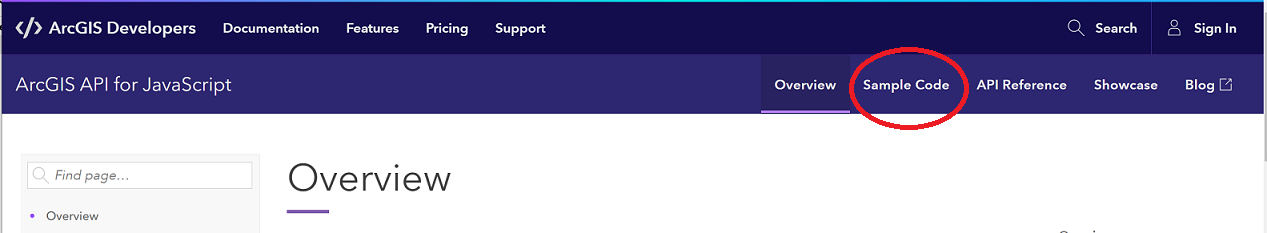 Figure 4.1 Accessing the Sample Code area of the ArcGIS Javascript API SDK
There you should see a list of Get started... samples. - Click on the Intro to MapView (2D) link. Like the other Samples pages, you should see a map embedded at the top of the page. Beneath the map, you should see buttons labeled Explore in the sandbox, Open in CodePen, View live and Download ESM sample.
- Click the Open in CodePen button. CodePen shows you the same map you just saw at the bottom of the page and the source code that produces that map on the top. The size of the "Preview" panel can be adjusted by dragging the horizontal bar separating that panel from the source code panels up or down. The power of CodePen is the ability to modify the source code and quickly see the result.
CodePen is built to encourage the separation of HTML, CSS, and JS code (a good development practice) with separate panels for each. However, note that it's OK to include CSS and JS in with the HTML, which is what happens when you open an Esri sample in CodePen.
Also note that it's possible to reconfigure CodePen such that the code panels are on the left or right rather than on the top. (I prefer having them on the left and the Preview panel on the right.) Making this change is done by clicking the Change View button (found next to the Settings button).
The sample is coded so that the map is centered over Scandinavia at a zoom level of 4. What if you wanted to display the United States instead? That’s easy! - Modify line 30 (or thereabouts - as the documentation does occasionally get updated) so that the MapView’s center property is set to a lon/lat array of [-95, 40]. You should see that the Preview panel automatically updates as you edit the code. I find this to be annoying when working on map pages, so I go into Settings > Behavior, and toggle the Auto-Updating Preview setting to off. When making this setting, you'll need to click the Run button to see the result of your code changes.
Now, let’s say you wanted to use a different basemap. - Change line 23 so that the Map’s basemap property is set to "terrain" and again click the Run button. As you can see, the CodePen sandbox makes it very convenient to “play around” with the code samples.
Note: We’ll see shortly how you’d know what other values can be used to set the basemap property.
4.2 Use the API to Create Your First 3D Map
4.2 Use the API to Create Your First 3D Map
An exciting feature of version 4 of Esri's JavaScript API is its support for 3D scenes. Let’s have a look at a basic 3D sample.
- Go back to the Sample Code Overview page and click on the Intro to SceneView (3D) link.
- Using the same approach that you used for the 2D map, view the sample code in the CodePen sandbox and change the map’s center to the same coordinates and the scale to 4000000.
Note: Most of you have probably explored a 3D map like this one, though you may not be aware of all of the navigation options available to you. Read about the various mouse and keyboard controls and their associated effects in the documentation of the SceneView class, and be sure to try them out!
Also note that in addition to the Open in CodePen option, the sample pages also offer an Explore in the sandbox option. This is Esri's own sandbox for experimenting with their samples, much like CodePen.
4.3 Separate Your HTML, CSS and JS Source Code Using CodePen
4.3 Separate Your HTML, CSS and JS Source Code Using CodePen
The samples in the SDK are written with the CSS and JavaScript code embedded within the HTML code. This is fine for simple apps, but for more complex apps it is recommended that you write the CSS and JavaScript in separate files. Among the benefits to this approach are:
- improved organization, making it easier to find your CSS or JS code rather than having to hunt in your HTML code for it;
- the ability to reuse code that is applicable across projects;
- shorter page load time through caching of the external files; and
- the ability to “minify” the code, making it a smaller download for client devices.
Let's revisit the Intro to MapView (2D) sample in CodePen, looking to follow a code separation approach.
- Return to CodePen. (Here's the CodePen homepage if you no longer have the earlier samples open.)
- If you don’t yet have a CodePen account, click the Sign Up button and supply the info needed to establish a free account.
After signing up, your browser window should open up to a new Pen (environment for authoring a new web page). - Click the Change View button in the upper right and select your preferred Editor Layout option.
- Click the Save button. This will give your pen a randomly generated name (in the upper left).
- Click on the pencil icon to the right of the pen name and assign it a new name of hello_map.
- Go back to the Intro to MapView (2D) sample sandbox. Copy and Paste the three components of the sample into their respective panels in CodePen. Note the following:
- You should omit the DOCTYPE declaration from the HTML piece.
- Do not include the style and script tags surrounding the CSS and JS code, respectively.
- Make sure that the <script src=....></script> tag is in the HTML window
- You may find it most convenient to copy the complete sample (CSS and JS included) to the HTML panel, then cut and paste the CSS and JS pieces to their respective panels. (You can remove the empty style and script elements from your HTML when done.)
- The code panels are resizable; if you’ve set the Editor Layout such that the code panels are arranged vertically to the side of the Preview panel, note that you can double-click on any of the panel headings to maximize that panel.
4.4 Move Your Code to .html, .css, .js files
4.4 Move Your Code to .html, .css, .js files
Playgrounds like Esri’s JS SDK sandbox and CodePen are great tools for experimenting with samples and developing your own apps from scratch, but when you want to “go live” with an app so that others can use it, you’ll want to host your code on a web server. You used a web hosting service in the previous lesson and we’re going to use that service again now.
When building apps, a convention that many developers follow is to create a folder on the web server for their site/app and into that folder place an HTML file called index.html (or default.html). For example, in building my “app_to_end_all_apps” site, I’d create a sub-folder by that name in my www folder, then upload my app’s HTML markup in a file named index.html to that sub-folder. I could then view my app using the URL: http://detwilergeog863.000webhostapp.com/app_to_end_all_apps/. (Note: This app doesn't actually exist, so you should expect a File Not Found error if you follow the link.) I could omit the index.html from the URL since browsers are built to look for a file by that name when the URL ends in a folder.
- On your computer, wherever you’re storing your coursework, create a folder called hello_map. (The name for this app is a play on computer programming's "Hello, World" tradition.)
- Create a new blank text file, copy your HTML code from CodePen into that file, and save it as index.html in your hello_map folder. Be sure to add a <!DOCTYPE html> line at the top of the file to declare your code as HTML 5.
- Create another blank text file, copy your CSS code into that file, and save it as main.css, again in the hello_map folder.
- Finally, create a third text file for your JS code. Call it main.js.
Unlike the CodePen environment, the end user’s browser won’t know that there is a CSS file and a JS file that goes along with the HTML file unless you tell it. - To reference your CSS code, add the following line above the line that references Esri’s main.css stylesheet:
<link rel="stylesheet" href="main.css"></link>
- To reference your JS code, add the following line after the line that references Esri’s JS API:
<script src="main.js"></script>
Note: These references use relative paths to locate the files; the browser will look for the files in the same folder as the HTML file since no folders were included in the paths. Because the architecture of this app is not particularly complicated, I’m directing you to store all of the files together. But you should keep in mind that many developers prefer to store their files in sub-folders (e.g., css/, js/ or styles/, scripts/) for organizational reasons. - Open this local copy of your app in a browser (right-click on the file in Windows Explorer and select Open with). As you develop your app, you can leave it open in your browser and Refresh (F5) whenever you want to see the result of your changes.
- To publish your app to a public facing location, open a connection to your www space on the 000webhost web server (using either FileZilla or the 000webspace File Explorer).
- Replicate the directory structure you have locally by creating a folder called hello_map.
- Upload the three files associated with the app to that folder.
- Test the app by pointing your browser to surnamegeog863.000webhostapp.com/hello_map, replacing surnamegeog863 with your website name.
For extra practice, go through the process of copying the 3D sample code to CodePen and then create a site called hello_scene in your web space.
4.5 Dissecting the Esri Samples
4.5 Dissecting the Esri Samples
Now that you’ve had a chance to dive right into building your own map apps, it’s time to learn more about what’s happening in those apps before you can go further with the API. Let's examine these start-up pages and discuss their HTML, CSS and JS pieces, beginning with the HTML of the 2D sample. Be sure to open up each of the three files so you can follow along with the discussion.
4.5.1 The HTML
4.5.1 The HTML
After completing the previous lesson, you should recognize the <html>, <head> and <body> tags. You should also recognize that the <!DOCTYPE> directive declares that the document is written as HTML 5.
The <head> of the document contains two <meta> elements. The second of these is concerned with rendering the document in a user-friendly way across a variety of devices (part of the larger CSS topic of responsive web design). This is not critical for you to worry about now, but you may want to return to this topic if you are developing for mobile phones or tablets. The first meta element specifies that your document is encoded in the UTF-8 character set, one that supports all of the world's major languages. It's a good idea to include this line verbatim in all of your map pages. If you're an insomniac, you may want to read more about character encoding.
The <head> also contains the page’s title, links to two external stylesheets (your own main.css file and Esri’s main.css file), and two script elements (one referencing the Esri JS API and the other your local main.js file). We’ll discuss the CSS and JS source code in detail shortly.
Next in the HTML file comes the body of the document, in which the only thing you'll find is a div element. This element is used to create a division, or section, in a document. In a web mapping context, a div is typically used as the container for the page's map. Note that this div is assigned an id (viewDiv).
4.5.2 The CSS
4.5.2 The CSS
Looking at your main.css file, there are three elements being styled: the html element, its child body element, and the element having the id of viewDiv (indicated by the pound sign). Each element has four property settings applied to it. The height and width settings specify that the element should take up all of the space of its parent container. The padding and margin settings specify that there should be no white space inserted on the inside or outside of the element, respectively. Basically, these styles produce a map filling the entire browser window.
4.5.3 The JS
4.5.3 The JS
Learn More
At this point, you should familiarize yourself with the syntax of JavaScript (JS). The w3schools site offers a good hands-on JavaScript tutorial that should do the job. Take a couple of hours to work through the topics listed under the JS Tutorial heading and pay particular attention to the following points:
- Ending statements with a semicolon is optional. (The Esri samples use them.)
- Note the difference between placing JS code inside the page's head section and its body section. See also this discussion of JS code placement.
- JavaScript is a dynamically typed language; you do not need to specify a data type when declaring a variable.
- JavaScript variables are case sensitive.
- Variables can be initialized on the same line that they are declared.
- Code associated with a conditional statement (if or else statements) or a loop (for or while) must be enclosed in braces.
- Alert boxes can be used to debug scripts that aren't working properly.
- JS functions are reusable blocks of code with an optional return value.
- The backslash (\) can be used to insert special characters in a string (e.g., if you want a string enclosed in double quotes to also contain a double quote).
- Comments are signaled in JS using two slashes (//).
Now that you've learned a bit about JavaScript, we can examine what’s happening in the main.js file.
AMD
The first thing you should notice is that all of the code is wrapped inside a require() function. This is a result of the fact that Esri’s API is built around a JS toolkit called Dojo. Dojo uses a design pattern called Asynchronous Module Definition (AMD) to load JS resources into memory. By defining their API’s object classes in modules, Esri’s made those classes easier to maintain and re-use. Loading the modules asynchronously (in parallel rather than one at a time) means that apps built on the API will load faster than they would in a non-AMD framework. One of your recurring tasks as an Esri JS developer will be to identify the modules containing the object classes needed by your app.
In the case of the 2D sample, two Esri classes are needed: Map and MapView. These classes are accessed by loading the esri/Map and esri/views/MapView modules, respectively. The list of modules at the beginning of the require() function is then followed up by an anonymous callback function. The function is anonymous, in that it has no name. It’s a “callback” function because Dojo's module loader will call back to the function when it's done loading the modules, passing module references to the function.
In order to work with the classes held in the modules being loaded, the callback function contains a list of parameters that corresponds to the list of modules. In the 2D example, only the esri/Map and esri/views/MapView modules are required, so the only parameters defined in the callback function are Map and MapView. We’ll see other parameters associated with other modules in more complex examples later. Some notes on the callback function parameters:
- The module loader will pass the module references as arguments to the callback function in the same order that the modules were listed.
- The naming of the parameters is up to you, though the accepted practice is to name them the same as their corresponding modules.
- As with parameters in any JavaScript function, you can go on to use the parameter as desired in the body of the function.
In the 2021-22 time frame, Esri's samples switched to a "fat arrow" syntax for function declarations. For example:
require(["esri/Map", "esri/views/MapView"], (Map, MapView) => { }
This syntax is a bit more concise than the previously used syntax:
require(["esri/Map", "esri/views/MapView"], function (Map, MapView) { }
I've attempted to update my own examples to be consistent with Esri's change, but you may still see the old syntax in places. If so, no need to worry. They are equivalent syntaxes for declaring a function. You'll also see some of Esri's samples using the old style too.
The DOM
An important web browser technology relied upon by Esri's JS API is the Document Object Model, or DOM. This is a tree-like representation of a web page that the browser creates whenever it loads that page. The DOM provides the means for JS developers to manipulate a page’s contents and behavior programmatically. In the case of developing an Esri JS app, the DOM is needed to insert a map or scene onto the page. SInce the require() callback function references DOM objects, it is critical that the DOM is loaded before the callback executes. However, we don't have to worry about this because require() has built-in functionality that waits for the DOM to finish loading before executing the callback function.
Code samples in older incarnations of the API documentation included another module called domReady! This is a Dojo module that is used to ensure that none of the code that follows in the callback function is executed until the DOM has finished loading. The fact that Esri removed references to domReady! in their samples implies that there's no longer -- or never was -- a need to worry about the callback function code executing before the DOM was done loading. In any case, I mention it here in case you run into it either in Esri's or this class's samples. Since the domReady! module -- also referred to as a plugin in Dojo's documentation -- doesn't have a meaningful return value, you'll note that it doesn't have a parameter to go with it in the callback function parameter list.
Learn More
Once again, the w3schools site offers a good JavaScript HTML DOM tutorial. This short tutorial should only take you 30-60 minutes to complete.
Using the API Reference
Earlier in the lesson, we visited the Esri JS API SDK to locate sample code that could be used to create our first apps. Now, let’s have a look at an equally important part of the SDK: the API Reference. The API Reference contains a list of all the API modules down the left side of the page. Each module heading can be expanded to see the classes defined in that module. For example, we’d find the Map class in the esri module and the MapView class in the esri/views module.
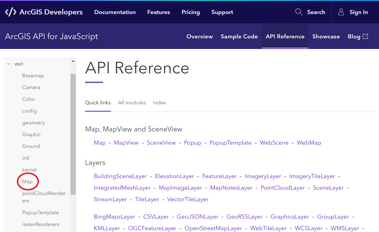
On the right side of the API Reference index page is a list of commonly used classes, generally organized from top to bottom in order of importance. We’ll cover most of these classes over the course of the term.
The first line of JS code in our 2D sample creates an object of the Map class (new Map). We can learn about that class by clicking the Map link on the API Reference index page or by entering Map into the Find page box.
Like the other class description pages in the API Reference, the page for the Map class conveys a lot of useful information:
- how you’d go about referencing the class in your code’s require() declaration
- an overview of the class (what it’s used for, a code snippet showing its usage, and links to samples and related classes)
- the class’s constructors (more on this shortly)
- the class’s properties (characteristics that uniquely define Map objects)
- the class’s methods (actions that the Map class is programmed to perform)
The Properties section of the page includes an Overview, listing all of the properties in alphabetical order along with their type (e.g., String, Number, or some object class). The property type is important to know as it tells you what you can expect to get back if you read the property (or conversely, what you need to supply if you’re setting the property). After the Overview, you’ll find a section of Details, providing more specifics on the class’s properties. For example, the details on the basemap property provide a list of acceptable values, along with a thumbnail of each.
The Methods section likewise includes both an Overview and Details section. Method parameters (pieces of information the method uses in performing its action) are listed in parentheses after the name in the Details section. If a parameter is optional, it will be listed with a question mark next to it. If a method returns a value when it is called, the method parameters will be followed by an arrow symbol pointing to the return type. Looking at the Map class methods, the add() method has a required parameter (layer), an optional parameter (index, specifying the position in the Map’s layer collection where you want the layer to appear), and no return value. The findLayerById() method has a required layerId parameter and it returns a reference to a Layer object. Note that when a parameter or return value is an object, it will appear in the documentation as a link. This helps you to navigate through the SDK as you write your code.
The part of the class documentation that we glossed over was the Constructor section. This section is intended to provide guidance on how to create a new object of the class. This is done by using the word new followed by the name of the class and a set of parentheses. In some APIs (including version 3.x of Esri’s JS API), it is possible to set just certain properties of the object you’re creating as part of the constructor statement, making it important to consult the Constructor section of the class’s documentation. However, in version 4.x, any of the class’s properties can be set as part of the constructor, which is why you’ll note that the Map class constructor says simply properties? within the parentheses.
Whatever properties you decide to set in the constructor should be expressed as a JS object literal, a term that may seem intimidating, but is actually not too difficult to grasp. Object literals are basically a list of property-value pairs, in which the list is enclosed in curly braces and the property-value pairs are separated by commas. In the case of the 2D sample, the Map was constructed with just a single property-value setting (the basemap), whereas in the 3D sample, it was constructed with two property-value settings (the basemap and the ground).
Note that you need not set all properties as part of the constructor. For example, I could rewrite the 2D sample as follows:
const map = new Map();
map.basemap = "streets";
Or the 3D sample as follows:
const map = new Map({
  basemap: "streets"
});
map.ground = "world-elevation";
One last word on constructors... When creating an object, you’re typically doing so because you need it later in your script. Thus, you will usually store a reference to the object you’re creating in a variable. In the samples, the new Map object was stored in a variable called map. That variable was later used to set the map property of a MapView object. Having multiple entities in a script with the same name can be confusing, especially for beginners, so I like to assign variable names that don’t duplicate the name of a class or property. In this case, I might use myMap or theMap. Keep in mind though that this means updating other statements in which that variable is referenced:
require([
  "esri/Map",
  "esri/views/MapView"
], (Map, MapView) => {
  const myMap = new Map({
    basemap: "streets"
  });
  const myView = new MapView({
    container: "viewDiv",
    map: myMap,
    zoom: 4,
    center: [15, 65]
  });
});
And finally, one more aspect of the Esri samples that has changed over time is in the way references to objects are stored. In the past, the samples created variables to store references to objects using the var keyword. Today, you'll see that the samples now typically employ the const keyword in place of var. As you might have guessed, const is short for constant. It is called for when you want to store an object (or primitive value, such as a number or string) in memory for use later in your code, with the important caveat that a constant can never be reassigned a new object or value. That's in contrast to variables, which as the name implies, can be reassigned a new object or value (i.e., they're allowed to vary). In the short snippet above, for example, the const myMap and const myView statements were previously written as var myMap and var myView. Using var still works and is not wrong, but if myMap is always going to refer to the same Map object, it's more appropriate to declare it as a constant.
In thinking about the difference between const and var, it's important to note that while you can't assign a new object to a constant after you've declared it, you are allowed to set properties of the object to new values. In other words, if you were adding code to the snippet above, you would not be able to do this:
myMap = new Map({...}); //or const myMap = new Map({...});
but you could do this:
myMap.basemap = "terrain" //same object, just altering a property
If you really wanted to create a new Map object and store it in myMap -- recycling that space in memory, if you will -- you could certainly do that. You'd just need to declare myMap using var rather than const. Similarly, if you want to store the number 2 in x and later change x to 3, you would need to declare x using var rather than const.
Lastly, you'll see that the course text generally refers to all named spaces in memory as variables, even those declared using const. Technically, anything declared using const should be referred to as a constant, but the term variable is so commonly used in programming that I hope you will excuse the imprecise language. Just keep in mind that most of these named spaces are actually constants, not variables.
4.6 Maps, Scenes and Views
4.6 Maps, Scenes and Views
We’ve already been exposed to the Map, MapView and SceneView classes in experimenting with and discussing the Esri samples. Now, let’s learn some more about these fundamental classes.
In version 4.x of Esri’s API, the Map class is used to store a basemap and layers. The actual rendering of the Map on the page is done through the use of a View: either a MapView (2D) or a SceneView (3D). If you look back at the two samples we’ve been working with, you’ll note that a Map object is created and its basemap property set in both cases. The only difference is that in the 3D example, the Map’s ground property is set in addition to its basemap. Setting the ground property renders the map such that the underlying terrain can be seen. The property can be set to “world-elevation” to use Esri’s default world elevation service, but it is also possible to use other elevation layers. (Setting the ground property in a Map that is displayed in a MapView has no effect since the MapView class only renders Maps in 2D.)
The other commonly used property of the Map class is its layers property. We’ll look at adding layers to a map in depth later in the course.
Looking at the documentation of the MapView class, you’ll see that it contains a whole host of properties. The most commonly set MapView properties include:
- map: set to an object of the Map class
- container: set to a string matching the id of an element on the page (or to a reference to the element itself)
- center: set to an object of the Point class
- zoom: set to a number, typically ranging from 3 (small scale)-18 (large scale)
- rotation: set to a number ranging from 0 to 360 degrees to rotate due North
Note that while center and zoom are commonly used to specify the part of the Map that’s currently visible, it’s also possible to do so using the extent and/or scale properties. Take care that you’re setting these properties logically. As explained in the documentation, if both the zoom and scale are set, then the scale setting will override the zoom setting. Similarly, an extent setting will override any center, zoom or scale setting.
3D SceneViews have the same set of properties as listed above, with the exception of rotation.
While it’s typical for a page to contain just a single View, you should keep in mind that you’re not limited to that sort of layout. It is sometimes useful to employ multiple views on the page, as in this sample that contains both a MapView and a SceneView.
4.7 Adding Overlays to a View
4.7 Adding Overlays to a View
The maps we’ve created so far have been pretty boring, so let's spice it up a tiny bit by plotting a point. We’ll see later in the course how to display features stored in one of Esri’s vector data formats. What I’m talking about doing right now is how you’d display a small number of geometries (points, lines or polygons) whose coordinates you’ve hard coded into the app, or perhaps acquired through user input.
- Create a copy of your hello_map folder (and its files) called lesson 4.
- Set the HTML doc’s title to Plotting a point.
Adding geometries the way I’m describing here involves creating one or more objects of the Graphic class. - Look up the Graphic class in the SDK using the Search box. (The result you want is the class found in the esri/Graphic module.)
As the overview explains, important properties of the Graphic class are geometry, symbol, and attributes. Attributes are important in situations where you want the user to be able to click on the graphic and see information about it in a popup window. We’re going to keep this simple, so we’ll focus on just the geometry and symbol, starting with the geometry.
Looking at the geometry property's description, you should note that in order to set it, you need to use a Geometry object. - Click on the Geometry link to go to that class's documentation page.
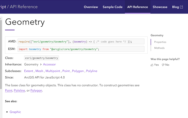 Figure 4.3 The Geometry class description in the API Reference
Its description tells you that it’s a "base class" and that it has no constructor. What this means is that you can’t create a plain Geometry object. You’d have to create a Point, Polyline or Polygon object instead. The Geometry class exists in the abstract as a way to define the properties and methods that the Point, Polyline and Polygon classes share in common (such as the extent property). (You might find it helpful to think of cars as an analogy. If you’re shopping for a new set of wheels, you don’t just buy a generic car; you buy some model of Ford, Toyota, Volkswagen, etc.)
In object-oriented programming terminology, the Geometry class can be described as the parent class or super-class of the Point, Polyline and Polygon classes (which are themselves child classes or sub-classes). These class relationships are conveyed at the very top of the class pages in the SDK. (Look for the Inheritance and Subclasses headings.) It turns out that you’ll find all of the properties and methods the Point, Polyline and Polygon classes inherit from Geometry on their pages. Not all SDKs are written this way (i.e., the SDK could have been organized such that you’d have to view the property and method lists on both the Point and Geometry pages to know all Point capabilities). - Getting back to our task, we know we want to add a point to the map, so follow the link to the Point class.
The Point class has several properties, but the ones we want here are latitude and longitude. - To the bottom of your JS code, add the following:
const pt = new Point({
  latitude: 40.792,
  longitude: -77.871
});
We’ve created a Point geometry for our Graphic, but have we forgotten something? Yes, if we want to work with the Point class, we need to include a reference to its module in our require() declaration. - Move to the top of your JS code and add "esri/geometry/Point" to the module list, then add Point to the callback function argument list (making sure you match its location in the list with the module’s location in the module list).
- With the Point geometry created, let’s move on to the symbol. In the SDK, make your way back to the Graphic class’s property list.
The symbol property must be set using a Symbol object. Following the Symbol link, you should note that, like the Geometry class, Symbol is an abstract parent class for several child classes. We’re trying to symbolize a Point here, so the subclass we need is MarkerSymbol. (We’d need LineSymbol for a Polyline and FillSymbol for a Polygon.) - Follow the MarkerSymbol link in the list of subclasses.
Reading over the MarkerSymbol class description, you should note that it is itself another abstract parent class, having subclasses PictureMarkerSymbol and SimpleMarkerSymbol. If you wanted to depict the point using some kind of graphic stored on disk, then you’d use the PictureMarkerSymbol class. We’ll keep our app simple by using the SimpleMarkerSymbol class, which will allow us to choose from a set of predefined shapes and apply a desired color and size.
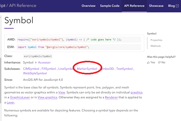 Figure 4.4 Accessing the MarkerSymbol class in the API Reference
 - Follow the SimpleMarkerSymbol link in the list of subclasses. Read over the class description and note the color, size and style properties.
- Create a new SimpleMarker as follows:
const sym = new SimpleMarkerSymbol({ color: "blue", style: "square", size: 12 }); - Update your require() declaration so that this newly added SimpleMarkerSymbol code will execute properly. Hint: the information you need is at the top of the class page in the SDK.
- With the geometry and symbol created, we’re ready to create a new Graphic object:
const ptGraphic = new Graphic({ geometry:pt, symbol:sym }); - We saw earlier in the lesson that the Map class has a method called add() for adding a layer. One way we could accomplish our goal here would be to add this Graphic to a new GraphicsLayer, then add the GraphicsLayer to our Map. However, a slightly easier alternative is to take advantage of the fact that the MapView has a graphics collection associated with it. We can simply add our Graphic to that collection as follows:
view.graphics.add(ptGraphic);
- Be sure to modify your require() declaration so that the browser will be able to find the Graphic class you just referenced.
- Test your app and confirm that a blue square is added to the map.
With that, you've reached the end of this lesson's content. Move on to the next page to access the assignment associated with this lesson.
Assignment: Plot Your Hometown
Assignment: Plot Your Hometown
The coding assignment for this lesson is in three parts. Here are some instructions for completing the assignment.
Part I
In an earlier course in our curriculum, you may have learned about the United States Geological Survey's Geographic Names Information System and the Getty Thesaurus of Geographic Names (for places outside the U.S.). Use those tools or any other resources at your disposal to locate the latitude/longitude coordinates of your hometown. (One handy way to get a location's coordinates is to pull it up in Google Maps, right-click on the location and select What's Here?)
Modify the lesson4 app code from earlier in the lesson so that the map is centered on and a marker points to your hometown. The easiest approach to this problem would be to insert your hometown coordinates in both lines of the script where coordinates are found. However, I hope you'll recognize that repeating values in different parts of a program is generally a bad practice because of situations like this where you end up having to make revisions in multiple places. So, while you're changing the location displayed on the map, revise the code so that it is as efficient as possible.
Part II
As you know, one way that web maps convey information to the user is through popup windows. We saw in Lesson 1 that layers can have popups configured using GUI-based tools in ArcGIS Online. In the next lesson, we'll see how the API makes it possible to easily incorporate layers and maps configured in ArcGIS Online into an app. And later we'll see how to configure layer popups programmatically. In this lesson, we've dealt with graphics, which don't have an attribute table associated with them. However, it's still possible to code the display of popups when the user clicks on a graphic.
For Part II, I'd like you to create a copy of the app from Part I and modify it so that clicking on a town marker will display some information about it (e.g., its name, population, when it was established, etc.). We haven't covered how to do this, but it is something that's demonstrated in an Esri code sample. You might be tempted to search the Sample Code area of the SDK for "popups," but all of the samples with that tag involve data layers rather than graphics. The sample I'm thinking of can be found under Graphics in the list of Sample Code categories.
Part III
Create a pen in CodePen that contains your code from either Part I or Part II (your choice).
Deliverables
This project is one week in length. Please refer to the Canvas course Calendar for the due date.
- Post the app containing your hometown map to your e-portfolio. (30 of 100 points)
- Post the app that displays popup info for your hometown to your e-portfolio. (30 of 100 points)
- Provide a link to your CodePen map -- or embed the pen itself -- in your e-portfolio. (20 of 100 points)
- Below one of your maps (or on your e-portfolio index page), include some reflection on what you learned from the lesson and/or any concepts that you found to be confusing (minimum 200 words). (20 of 100 points)
- Click on the Assignment 4 Submission to submit a link to your project page. (A link to your e-portfolio index page is OK too if it contains a link to your project.)
- Complete the Lesson 4 quiz.
Note: The examples you've seen so far are all likely to have shown the div element used to display the map/scene filling the whole browser window. You could add your reflection text beneath that div, but the map would still fill the whole window and it may not be immediately clear to the viewer that there was content below the map. It's probably a better idea to shrink the height of the map div to something less than 100%. If you're unsure how to go about this, here is an example that demonstrates one approach to including text on the page with the map.
Summary and Final Tasks
Summary and Final Tasks
In this lesson, you built your first apps using Esri's JavaScript API. Even the simple map that you created involves a number of different technologies (HTML, CSS, JavaScript, the Document Object Model, and the Dojo JavaScript framework) and it is important that you have a firm understanding of this material before moving on. If you skipped over the w3schools tutorials referenced in the lesson, be sure to go back and complete them. You might also use any free study time to work through other JavaScript references such as the ones recommended in the syllabus.
In Lesson 5, you'll see how to spice up the rather dull product of Lesson 4 by adding data layers. You'll also learn about a number of coding tools and strategies that will help you as a JavaScript developer.
Lesson 5: Adding Layers
Overview
Overview
So far in the course, you've spent the bulk of your time learning about the various web technologies that are involved in the creation of even the simplest web map applications. The last project deliverables were fairly basic, and you're probably itching to create apps that involve layers of your own data. In Lesson 5, we'll see how to create apps that incorporate web maps configured in ArcGIS Online and how to add various types of data layers to a map using Esri's JS API. We'll finish with a discussion of some coding tips now that you've gotten your feet wet with web app development.
Objectives
At the successful completion of this lesson, students should be able to:
- incorporate web maps (like in Lesson1) and web scenes into a JS app;
- use autocasting to avoid explicitly importing certain modules;
- understand how the REST web services protocol works;
- add various data layer types to a map;
- employ strategies to debug apps that aren't working properly;
- identify features in integrated development environments (IDEs) that aid in the coding process.
Questions?
If you have any questions now or at any point during this week, please feel free to post them to the Lesson 5 Discussion Forum. (That forum can be accessed at any time by clicking on the Discussions tab.)
Checklist
Checklist
Lesson 5 is one week in length. (See the Calendar in Canvas for specific due dates.) To finish this lesson, you must complete the activities listed below. You may find it useful to print this page out first so that you can follow along with the directions.
| Step | Activity | Access/Directions |
|---|---|---|
| 1 | Work through Lesson 5. | Lesson 5 |
| 2 | Complete the three-part project on the last page of the lesson.
|
Follow the directions throughout the lesson and on the Assignment page. |
| 3 | Take Quiz 5 after you read the online content. |
Click on "Lesson 5 Quiz" to begin the quiz. |
5.1 Incorporating Web Maps and Web Scenes
5.1 Incorporating Web Maps and Web Scenes
Back in Lesson 1, you created a web map of the Jen & Barry’s scenario data in ArcGIS Online, then incorporated that web map into an app using Esri’s three app building options that require no coding: embedding within a website, using a configurable app template, and using the Web AppBuilder. It turns out that even if you are coding your app, it’s quite easy to incorporate web maps like the one from Lesson 1 into your app. In fact, while the API provides the ability to configure your app programmatically (adding layers, symbolizing them, configuring popups, etc.), even the best coder is likely to find it helpful to use the ArcGIS Online GUI to reduce their coding burden.
5.1.1 Load a Web Map Into a 2D App
5.1.1 Load a Web Map Into a 2D App
In Lesson 1, we saw that it's possible to use the GUI-based tools in ArcGIS Online to author web maps that can then be easily incorporated into apps created using a configurable app template or the Web AppBuilder. It's also quite easy to do the same for apps developed using the JS API. Here's how:
- Copy one of your apps from Lesson 4 and name it jen_and_barry_2d.
- In the JS API SDK, browse to Sample Code > Mapping and Views > MapView (2D) > Load a basic web map > Explore in the sandbox.
This sample works by creating an object of the WebMap class and setting its portalItem property to a JS object defined simply as an id of a particular value. That WebMap is then used to set the map property of the MapView (in place of the plain Map object we saw in the previous lesson). Note the reference to “esri/WebMap” in the require() declaration.
Adapting this sample to your own liking is as simple as setting the portalItem’s id property to that of your own web map. - Copy the sample’s JS code into your own jen_and_barry_2d main.js file replacing your content with the sample's.
- In ArcGIS Online, browse to your web map from Lesson 1 and open it in the map viewer.
- In your browser’s address bar, you should see a URL ending in “webmap=” followed by a long alpha-numeric string. Copy that string to your clipboard. (Double-clicking somewhere on the string should select it.)
- Paste the string into your main.js file, replacing the portalItem id value from the sample.
- Test your app by opening it in a browser.
Two important points to keep in mind about consuming web maps:
- The map can be stored in ArcGIS Online as we saw here, or in your own organization’s ArcGIS Portal instance.
- You’ll want to make sure that the map has been shared with your intended audience; otherwise, it will not appear.
5.1.2 Load a Web Map Into a 3D App
5.1.2 Load a Web Map Into a 3D App
We saw in the previous lesson that a Map can be associated with a MapView to produce a 2D app or with a SceneView to produce a 3D app. Likewise, a WebMap can be used as the basis for a 2D or 3D app.
Create a copy of your jen_and_barry_2d app and modify it so that your web map is displayed as a 3D app.
5.1.3 Load a Web Scene Into a 3D App
5.1.3 Load a Web Scene Into a 3D App
Thus far in the course, we’ve seen how to drape 2D data over a 3D globe, but we haven’t really taken advantage of the 3D environment yet. Web scenes are basically the 3D analog to web maps, in which the scene features have a Z component.
Web scenes can be either global, for situations where the earth’s spherical nature comes into play, or local, where it does not. Global scenes are displayed in the Web Mercator coordinate system, whereas local scenes can be displayed in a local, planar coordinate system.
This example showing earthquakes is an example of a global scene. And this detailed model of a building and its interior provides an example of a local scene.
As with web maps, web scenes are published and discoverable through ArcGIS Online or through local implementations of ArcGIS Portal. This search will provide a list of scenes owned by Esri’s 3D team, including models of many world cities.
Have a look at the Load a basic web scene sample in the SDK.
Note that the only difference from the jen_and_barry_3d app you created earlier is in the use of the WebScene class in place of the WebMap class.
5.2 Autocasting
5.2 Autocasting
In looking at the Load a basic web scene sample (or perhaps earlier samples), you may have noticed a comment “autocasts as new PortalItem().” So what does that mean? Certain properties in the API have been coded behind the scenes by Esri so that our jobs are made a bit easier. Like all properties, the ones that support autocasting are written expecting to be set to a particular data type (e.g., string, number, object). Where these properties differ is that they can also be set to a JavaScript object that “looks like” the required object type. This is a concept that’s much easier to explain by example, so let’s work through what the Load a basic web scene code would look like if autocasting was not built into the API.
- Open the API Reference in the SDK and look up the WebScene class.
- Find the portalItem property and note that its data type is listed as PortalItem. Ordinarily this would mean that you’d need to create an object of that class (using new PortalItem) to set the WebScene’s portalItem property. And of course, that would mean adding the PortalItem class to your require() declaration. Here is how the code would need to look if autocasting was not available, alongside how the sample is actually coded:
| No autocasting used | Autocasting used |
|---|---|
require([
      "esri/views/SceneView",
      "esri/WebScene",
      "esri/portal/PortalItem"
    ], (
      SceneView, WebScene, PortalItem
    ) => {

      const myPortalItem = new PortalItem({
        id: "3a9976baef9240ab8645ee25c7e9c096"
      });

      const scene = new WebScene({
        portalItem: myPortalItem
      });

      const view = new SceneView({
        map: scene,
        container: "viewDiv",
        padding: {
          top: 40
        }
      });
    });
|
require([
      "esri/views/SceneView",
      "esri/WebScene"
    ], (
      SceneView, WebScene
    ) => {

      const scene = new WebScene({
        portalItem: {
          id: "3a9976baef9240ab8645ee25c7e9c096"
        }
      });

      const view = new SceneView({
        map: scene,
        container: "viewDiv",
        padding: {
          top: 40
        }
      });
    });
|
So autocasting makes it a bit easier to set certain properties. The way to tell which properties behave this way is to look for the word autocast next to the property’s data type in the class’s documentation.
Here’s a second example to drive the point home. In the previous lesson, we worked with the MapView class in creating simple 2D apps. In the samples we dealt with, the MapView center property was set using a syntax like this:
center: [-112, 38]
However, the documentation of the center property tells us that its data type is Point. Thus, if the property didn’t support autocasting, we’d need to add the Point class to the require() declaration and create a Point object using the class’s constructor. Here are three alternative versions of the Get started with MapView sample:
| No Autocasting used | Autocasting used | Autocasting used (with lon/lat array) |
|---|---|---|
require([
  "esri/Map",
  "esri/geometry/Point",
  "esri/views/MapView"
 ], (Map, Point,
MapView) => {

  const map = new Map({
    basemap: "streets"
  });

  const pt = new Point({
    latitude: 65,
    longitude: 15
  })

  const view = new MapView({
    container: "viewDiv",
    map: map,
    zoom: 4,
    center: pt
  });
});
|
require([
  "esri/Map",
  "esri/views/MapView"
], (Map, MapView) => {

  const map = new Map({
    basemap: "streets"
  });

  const view = new MapView({
    container: "viewDiv",
    map: map,
    zoom: 4,
    center: {
      latitude: 65,
      longitude: 15
    }
  });
});
|
require([
  "esri/Map",
  "esri/views/MapView"
 ], (Map, MapView) => {

  const map = new Map({
    basemap: "streets"
  });

  const view = new MapView({
    container: "viewDiv",
    map: map,
    zoom: 4,
    center: [15, 65]
  });
});
|
The first version is the syntax we’d need if autocasting was not available on the center property. The second uses autocasting as we saw in the PortalItem example above. The third is how the sample is actually written in the SDK. Unlike the PortalItem example, the property is set to a JavaScript array rather than a JavaScript object. This appears to be a special case supported by the MapView center property. In general, you should use an object, not an array, when working with an autocast property.
5.3 REST API
5.3 REST API
Thus far in the course, the apps we’ve built have consumed map services hosted by Esri on their ArcGIS Online platform. Another common source for map services is ArcGIS Server. Many organizations, in both the private and public sectors, implement their own instances of ArcGIS Server as a means of publishing their geographic data. The JS apps built by these organizations typically consume their own services.
Esri makes it possible to consume their web services through the two primary architectural styles employed by web developers today: SOAP (Simple Object Access Protocol) and REST (REpresentational State Transfer). The SOAP protocol was developed by Microsoft in the 1990s and can be thought of as object-oriented programming in which the objects live on some web server and the programming code that manipulates them lives on some client machine. REST came later and has overtaken SOAP in popularity because of its ease of use. RESTful web services, as they are sometimes called, progressively expose their functionality through URLs that can be invoked almost like properties and methods. They send responses to the client applications in the form of XML or JSON.
One important aspect of using this framework is that information on the various REST web services published through an ArcGIS Server instance can be discovered through a series of pages called the Services Directory. This directory can be viewed in a web browser using a URL of the form <server name>/arcgis/rest/services.
Developers working with services published through ArcGIS Server do so using Esri’s REST API. Esri had their own short (3-hour) web course that did a nice job of explaining how to use the REST API. They retired that course, but I did manage to capture the written lesson content from it -- Esri Training: Introduction to the ArcGIS for Server REST API (as PDF). Please work through this document, paying particular attention to the parts of the course dealing with layer services, as that is what we’ll be focusing on in this lesson.
You should also be sure to consult the documentation -- ArcGIS Resources: REST API.
5.4 Layer Types
5.4 Layer Types
ArcGIS Server publishes data layers of several different types, depending on whether the underlying data source is vector or raster, the amount of data being served, the needs of the apps consuming them, etc. In this part of the lesson, we’re going to walk through the most commonly used types, describing how they differ from one another, how they can be distinguished from layers of other types, under what circumstances they’re intended to be used, and how they are incorporated into an app.
In a moment, we'll take a detailed look at the most useful layer types one by one. Before doing so, here are some important properties that are defined under the abstract Layer class that is the parent to all of the layer sub-classes:
- opacity: set to a value from 0 to 1, with 0 making the layer completely transparent and 1 making it completely opaque (solid),
- title: set to a string specifying how the layer is labeled in widgets like the Legend and LayerList,
- visible: set to a Boolean controlling whether or not the layer is turned on/off.
5.4.1 TileLayer
5.4.1 TileLayer
Description:
- displays a full dataset using a series of adjacent tiles (smaller individual images that you can think of as snapshots of the complete map)
- a different set of tiles is created for each level of detail (zoom level)
- referred to as a cached service because the tiles are pre-created (i.e., not dynamically at the time the request for the layer is received by the server)
- can show data from many different underlying datasets at once
- often used as a basemap; in fact, most of the options when setting a Map’s basemap property result in the addition of a TileLayer
- changes in the underlying data cause the service to be out of date, so this layer type is best suited to data that changes infrequently
- tile creation can be a time consuming process; often automated to run overnight
- because you’re dealing with a picture of your data, you can’t implement popup windows
- can create your own using ArcMap or ArcGIS Pro (see GEOG 865)
How do I know I’m dealing with a TileLayer?
- labeled as a MapServer service in the REST Services Directory
- the service’s Single Fused Map Cache property will be true and it will have a Tile Info section
Class description in the SDK:
Example service:
Code sample:
- ArcGIS API for JavaScript: Get started with layers
- TileLayer objects are created and stored in the transportationLyr and housingLyr variables
5.4.2 VectorTileLayer
5.4.2 VectorTileLayer
Description:
- newer technology than raster tiles
- data are still cached, but aren’t just static pictures
- service passes geometry and styling info to client, which then does the rendering
- Attributes are not included, popups and other feature interactions are not available
- same set of tiles can be styled in many ways
- also mostly associated with basemaps; the -vector options of the Map’s basemap property result in the addition of a VectorTileLayer
- tile creation much shorter process than for raster tiles
- tile creation can be done in ArcGIS Pro, but not ArcMap
How do I know I’m dealing with a VectorTileLayer?
- unlike the other layer types described here, vector tile layers can only be discovered through ArcGIS Online or ArcGIS Portal
- in ArcGIS Online, when viewing the layer’s Details page, its Source will be listed as a Vector Tile Service and it will have a View Style button
Class description in the SDK:
Example service:
- several world-scale vector tile layers (all based on the same data, just styled differently) created by Esri and hosted on ArcGIS Online: ArcGIS Vector Basemaps
Code sample:
- ArcGIS API for JavaScript Sandbox
- note the layer’s url property can be set to the service itself (and drawn with default styling) or to a JSON style object; see ArcGIS API for JavaScript: VectorTileLayer
5.4.3 FeatureLayer
5.4.3 FeatureLayer
Description:
- feature geometry and attributes sent to client; rendered on client
- features to stream to the client are often filtered using a definition expression
- having the geometry and attributes on the client enables the implementation of popup windows
- also supports several types of renderings (e.g., unique values, class breaks, etc.)
How do I know I’m dealing with a FeatureLayer?
- on ArcGIS Server instances, can be created from a service labeled as either MapServer or FeatureServer
- when dealing with a service containing multiple layers, must create the FeatureLayer from one of the service sub-layers
Class description in the SDK:
Example service:
Code sample:
5.4.4 MapImageLayer
5.4.4 MapImageLayer
Description
- picture of your layer taken on the fly by the server and sent to client
- often a mix of different layers, each of which can be customized (renderer, definition expression, etc.)
- use if a FeatureLayer would be too much for client to handle
How do I create a MapImageLayer?
- On ArcGIS Server, instances can be created from a service labeled as MapServer
- can create from either the full service or a sub-layer
Class description in the SDK:
Example service:
Code sample:
5.4.5 ImageryLayer
5.4.5 ImageryLayer
Description:
- stream of raster data from the server to the client device
- raster can have pixel filtering and rendering performed on the server or client
Class description in the SDK:
Example service:
Code sample:
5.5 Coding Tips
5.5 Coding Tips
We'll end this lesson with some content that will hopefully make you a bit more successful as a coder. We’ll talk about development environments (where you write your code) and debugging tools. But first, here are a few tips that apply regardless of the kind of programming you're doing:
- Write your code in baby steps. Start with something very simple (or a working sample that you modify slightly), test it, add a small piece, test again, etc. Avoid writing long blocks of code without testing. The more untested code you write, the harder it will be to identify errors.
- When inserting an opening brace, bracket or parenthesis, insert the matching closing character at the same time. If you wait to do that until after you've finished entering the intervening statements, you're apt to forget.
- When the JavaScript console reports multiple errors, fix just the first error, then reload the page. One error can cause several others to appear downstream; fixing it can cause the rest to disappear.
- As with writing in general, the best way to get past a block is often to take a break and come back to the code later. With a fresh look at your code, it may take just minutes to find a bug that you had banged your head against the wall about for hours the night before.
5.5.1 Development Environments
5.5.1 Development Environments
Plain text editors like Notepad are OK for beginners getting to know web-publishing languages, but there are more advanced tools out there that make the developer's job easier. Integrated Development Environments (IDEs) are software applications that allow developers to write, test, and debug source code all in one application. IDEs also frequently provide auto-completion (i.e., a list of valid properties and methods available through an object) and syntax highlighting (i.e., different language elements shown in different colors/styles). Examples of popular IDEs include Microsoft Visual Studio and Eclipse. CodePen can be thought of as an online web programming IDE (as opposed to one installed on your own computer).
There are lots of IDEs suited for web development, as a web search for "web development ide" will show you. For the purpose of continuing on through this course, I'm going to recommend Notepad++. As its name implies, it's a step (or two) up from Notepad. My main reasons for pointing you to it are that it is free, it's easy to use, and it provides line numbers and syntax highlighting. Notepad++ is arguably not a true IDE since it's not possible to view your pages directly within the same application, but it does allow you to easily launch them in various web browsers, so I think that's a rather pointless debate.
Let's walk through a short set of steps to familiarize you with Notepad++.
- Download and install Notepad++.
- Open your hello_map app’s index.html page in Notepad++. An easy way to do this is to browse to it through your file system, right-click on it, and select Edit with Notepad++.
The first thing you should notice is the formatting applied to your code. HTML elements are shown in blue, attributes in red, and attribute values in purple. This happens because your file has a .html extension. Keep in mind that if you create a new page from scratch, you will not see this highlighting done until you save it with a .htm or .html extension.
Next, note the boxes just to the left of a few lines in your code. These boxes appear at the beginning of blocks of code that can be logically treated as a unit. - Click on the box next to the head start tag to collapse the code associated with the head element.
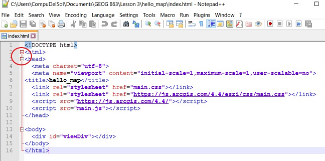 Figure 4.3 Collapsing the head section of an HTML doc in Notepad++
The minus that had been inside the box will change to a plus, indicating that clicking it again will re-expand that code unit. This is a feature of IDEs referred to as code folding. - Move your cursor down through the document and note that when the cursor is located within a start tag, that tag and its matching end tag will be highlighted (and vice versa). This highlighting can be very helpful, especially if you haven't done a good job of indenting your code logically.
- Now open the app’s main.js file in Notepad++ and move the cursor down the document until you reach the line where you create the Map object. Move the cursor to the right until you reach the opening brace. You should see that the brace is highlighted and a red line appears connecting the opening brace to its matching closing brace. The same behavior can be observed with brackets and parentheses. Given how often these characters are used in JavaScript -- and the importance of ordering them correctly -- this feature can be quite useful.
Now that we've worked with a more fully-featured source code editor, let's discuss some tips for working out the kinks in pages that aren't giving you the results you expect.
5.5.2 Debugging
5.5.2 Debugging
So, what do you do when you load your page in a browser and get...nothing? Thankfully, there are tools that can help pinpoint problems in your code without having to manually search line by line. Let's have a look at a couple of broken pages and how we can determine why they're broken.
- Load this Hello Map example in IE, Firefox, or Chrome. Your browser window should be blank because of an error in the page.
- Open the JavaScript console as follows:
Chrome - click on the menu icon (3 stacked dots to the right of the address bar), then select More Tools > Developer tools > Console.
Firefox - click on the menu icon (3 stacked lines, also in the upper right of the window) and select Web Developer > Web Console.
MS Edge - click on the menu icon (3 stacked dots, also in the upper right of the window), then select More Tools > Developer tools > Console.
You should see one of the following error messages, depending on your browser. (The console may report warnings in addition to errors, in which case you’ll need to skip over the warnings or toggle them off.)
Chrome - Uncaught SyntaxError: Unexpected identifier; the page's name and the line of the error appear to the right of the message (main.js:14, in this case)
Firefox - Uncaught SyntaxError: missing } after property list; main.js:14:4
MS Edge - Uncaught SyntaxError: Unexpected identifier; main.js: 14
Each browser in its own way is reporting that it encountered something unexpected on line 14. If this was your own page, you could have a look at that line in Notepad++ or whatever editor you are using. Let's just look at the source code in the browser in this case. - Within the Console, click on the main.js link listed next to the error message to view the code being loaded from that file. Depending on the browser you’re using, the code lines may be numbered. The "problem" line may also be highlighted or have the cursor on it. (If the .js code won't load in the Console, view the page's source code using Ctrl-U, then click the main.js link.)
As is sometimes the case, the problem here can be found just before the flagged line: there is no comma after the setting of the zoom property on line 13. It may seem confusing that the browser is flagging line 14, when the line requiring a fix is line 13, but it actually makes sense if you remember that a property-value setting doesn’t need to be followed by a comma (i.e., when it’s the last one associated with the object). So the browser flags the line where it’s finding something unexpected. (It expects a comma or closing brace after the zoom property.) - Load the second Hello Map example in IE, Firefox, or Chrome. Again, your browser window should be blank because of an error in the page.
- Using the error checking steps outlined above, you should identify the following error:
Chrome - Uncaught SyntaxError: Unexpected token ); on line 17
Firefox - Uncaught SyntaxError: expected expression, got ‘)’; on line 17
MS Edge - Uncaught SyntaxError: Unexpected token ')'; line 17
Line 17 is a pair of closing parentheses followed by a semi-colon. It’s logical to assume the second parenthesis closes the require statement’s arguments and that the first parenthesis closes some other entity in the code block. However, if you were to look at the code in Notepad++, you would see that the IDE matches the first parenthesis character up with the require arguments and that the second parenthesis has no match. The fact that the second parenthesis isn’t matched up with the opening parenthesis on line 1 indicates a problem. It turns out the first parenthesis shouldn’t be a parenthesis; it should be a closing brace (to go with the opening brace on line 4 defining the beginning of the callback function).
While checking for errors in this way can often be a big help, there are likely to be times when you're unable to identify the problem in your code. Another method for pinpointing problems is to produce some output at strategic points in your code. This could be as simple as an alert() statement that confirms that code execution reached a certain point, like
alert("Finished adding overlays");
You might also use an alert() box to display the contents of a variable or the property of some object:
alert("The coords are: " + pt.latitude() + ", " + pt.longitude());
An alternative to using alert() in this way is to write messages to the JavaScript console. This is especially preferable when you want to diagnose a problem with a loop and would rather not have to dismiss alert() boxes repeatedly. Writing messages to the console can be done as follows:
console.log("The value of i is " + i);
Over years of web development, I have found that these simple debugging strategies usually lead me to finding and fixing my errors.
5.5.3 JSLint/JSHint
5.5.3 JSLint/JSHint
One strategy for avoiding errors when you test your apps in a browser is to catch those errors in your development environment. A linter is a tool that is used to analyze code for potential errors before execution. Linters exist for many programming languages, but in a JavaScript context, JSLint is perhaps the best known. You can use JSLint online by navigating to JSLint, pasting your JS code into the big text box and clicking the JSLint button.
JSLint was developed by Doug Crockford in 2002 and the standards his linter enforces are described on the JSLint website. Many have found some of the JSLint rules to be overly strict (e.g., statements within a function are required to be indented exactly 4 spaces). For this reason, a more flexible alternative was developed as a community-driven open-source project: JSHint.
Many IDEs come equipped with one or both of these tools. Others can have the tools added through a plugin. Notepad++ had a JSLint plugin, but it does not work with the 64-bit version of the IDE (which you're likely to have installed). CodePen provides an Analyze JavaScript option on the JS editor panel's dropdown menu that is based on JSHint.
Pay attention to the availability and implementation of JSLint/JSHint in the IDE review portion of this week's assignment.
5.5.4 Beautifiers
5.5.4 Beautifiers
Especially when cobbling together snippets of code from various samples, it’s common for your code to become messy (e.g., indented inconsistently, varying amounts of whitespace, etc.). IDEs typically provide ways to indent or unindent blocks of code. In Notepad++, this can be done by highlighting the incorrectly indented code and hitting Tab or Shift-Tab, respectively. However, there are also beautifying tools available both online and within IDEs that can correct multiple kinds of errors across an entire document in seconds.
Here is a messy version of the Hello_Map JS code:
require([
    "esri/Map",
    "esri/views/MapView"
], (Map, MapView) => {

const map = new Map({
    basemap: "streets"
});


                const view = new MapView({
            container: "viewDiv",
            map: map,
            zoom: 4,
            center: [15, 65]
        });

});
This code, while perfectly valid as seen by browsers, is difficult for people to read because of the inconsistent indentation and large block of whitespace.
- Point your browser to jsbeautifier.org.
- Copy the messy code above and paste it into the large textbox on the jsbeautifier site.
- Click the Beautify JavaScript or HTML button either above or below the text box (or hit Ctrl-Enter). Voila! The messiness of this code is cleaned up.
There are several settings in the upper right of the page that you can use to tweak how the beautifier tidies your code. The first four dropdown lists are probably of the most interest:
- The first allows you to specify the number of spaces you wish to indent with (or use 1 tab instead). It’s considered good practice to use either tabs or spaces, but not to mix the two in the same document. Developers often have strong opinions in the space vs. tab debate. I lean toward using spaces since a space occupies one character regardless of the app you’re using to view the code, whereas a tab could be shown as 2, 4 or 8 characters wide depending on the app.
- The second list has to do with the amount of whitespace you want to appear between blocks of code (e.g., between two functions, after a loop or conditional expression, or as in this case, between the definition of two object variables).
- The third list allows you to specify the maximum width of your code before it gets wrapped to the next line.
- The fourth list involves the positioning of braces. Some developers (myself included) prefer to position the opening brace that goes with a function or object constructor on the same line as its “control statement”. Others prefer that the brace be placed on its own line.
I encourage you to experiment with these options to see how they affect the formatting of your code.
As with the linting tools, IDEs sometimes include a built-in beautifying tool or can have one added as a plugin. The only tool that I’m aware of for Notepad++ is JSToolNpp. I’m not going to walk you through the use of this tool since I’m not crazy about how it formats object definitions. For example, it formats an object like this:
const map = new Map({
        basemap: "streets"
    });
whereas I’d prefer it to be formatted like this:
const map = new Map({
    basemap: "streets"
});
However, you are welcome to install and play with the tool if you like.
Finally, you should note that CodePen offers a beautifier on the JS editor panel's dropdown menu (Format JavaScript).
5.5.5 Style Guides
5.5.5 Style Guides
In the previous sections, we saw that both linting and beautifying tools can be customized based on personal preference. Application development often involves multiple coders contributing pieces to the end product. Editing application code, whether fixing bugs or adding additional functionality, is much easier when all of the code is formatted in the same way. When code jumps between different formats (i.e., style rules), the person trying to interpret the code is forced to waste valuable time adjusting his/her mindset to the different formats. And even in organizations in which team coding is not employed, it is rare that an application will only ever be modified by the original author. Coders go on vacation, leave the company, etc. For these reasons, many organizations go to the trouble of constructing a style guide – a set of rules that all of their coders will follow. Here is a JavaScript style guide used at Google:
Many of these rules are fairly advanced, but there should be at least a few you can grasp. For example, the guide's authors specify that all statements must be ended in a semi-colon even though you might be able to get by with omitting them. Multiline string literals should be constructed using string concatenation rather than the line continuation character. Under the Code formatting heading, you’ll find some of the personal preference items we discussed in the beautifying section. Opening braces should be found on the same line as what they’re opening, property settings in an object definition should be indented two spaces, etc.
If you work in an organization that already does JS development and you’re going to be joining a development team, you should look into whether there is a style guide you should be following. If you’re just starting a new team, it might be a good idea to put some thought into creating a guide.
Assignment
The coding assignment for this lesson is in three parts. Here are some instructions for completing the assignment.
Although we learned about adding WebMaps and WebScenes to our apps, for full credit on Parts 1 and II you will need to add layers to the Map as discussed in 5.4 Layer Types. This will be useful in the next lessons where we need to access layers for custom symbology, queries, and features.
Part I
The Transportation Planning and Programming (TPP) division of the Texas Department of Transportation has published vector tile basemaps for Texas as services through ArcGIS Online. Find one of these services and create an app that displays its data in a 3D scene, zoomed in to the City of Houston.
Hint: You can narrow down your search in ArcGIS Online to different content types like Maps, Layers, Scenes, etc. Some content types are broken into sub-categories as well. Use the ability to search by content type along with appropriate search terms to identify the correct service. (Make sure you're not searching only the Penn State group content!)
If you're unable to find the described service, create a 3D app that displays data from some other vector tile service for partial credit.
Part II
One of Esri's sample ArcGIS Server instances hosts a map service that contains U.S. cities, interstates, and state/county boundaries:
Build an app that displays just the county boundaries on a 2D map. In your solution, you should be taking a snapshot of the data on the server and passing that to the client rather than passing the features themselves. Be sure to read the documentation carefully for how to display just the county sublayer. It might be a good idea to display all of the sublayers first before attempting to filter out some of them.
Part III
In this lesson, you began using a relatively basic IDE, Notepad++. For the last part of this week's assignment, I'd like you to download and experiment with a different IDE (Visual Studio Code, Sublime, WebStorm, Eclipse, Netbeans, Komodo), then share your thoughts on it in a recorded video. Here are some detailed instructions:
- Please go to the Assignment 5 IDE Review Sign-up page in the Lesson 5 module in Canvas to sign up for an IDE. The sign-ups will be set up such that the IDEs receive more or less equal coverage. (If there's another IDE that you'd like to evaluate, check with the instructor first.)
- Limit your video to 5 minutes.
- In your demo, be sure to discuss the IDE features that were mentioned in the lesson. And feel free to talk about any interesting features that were not in the lesson. (If demonstrating the IDE, please use files from a previous assignment rather than this week's.)
- Give your thoughts on whether you plan to use the IDE instead of Notepad++.
Deliverables
This project is one week in length. Please refer to the Canvas course Calendar for the due date.
- Upload the JavaScript file associated with your TX DOT vector tile app. No need to include the HTML or CSS. Don't post this app to your e-portfolio. (40 of 100 points)
- Upload the JavaScript file associated with your county boundary app. No need to include the HTML or CSS. Don't post this app to your e-portfolio. (40 of 100 points)
- Post a link to your IDE evaluation video to the Lesson 5 Discussion Forum. (20 of 100 points)
- Complete the Lesson 5 quiz.
Summary and Final Tasks
Summary and Final Tasks
In this lesson, you saw how to incorporate a web map you created using ArcGIS Online tools into a JavaScript API app and how Esri's REST API can be used to interact with services published through ArcGIS Server. You also learned about the various layer types built into the API and the circumstances under which each type might be used. Finally, you learned about some more generic web development topics, including Integrated Development Environments (IDEs) and debugging strategies.
Knowing the different layer types found in Esri's API and how to add them to a map is an important first step. However, chances are you'll want to customize the symbology of your map's layers so that they convey the desired information more effectively. That will be the focus of Lesson 6.
Lesson 6: Layer Visualization
Overview
In the previous lesson, we looked at several of the different types of layers in Esri's API that can be added to a map. One of the most important tasks in building a successful geospatial web app is to render the map layers so that they effectively convey the desired information. That will be the focus of this lesson.
Checklist
Lesson 6 is one week in length. (See the Calendar in Canvas for specific due dates.) To finish this lesson, you must complete the activities listed below. You may find it useful to print this page out first so that you can follow along with the directions.
| Step | Activity | Access/Directions |
|---|---|---|
| 1 | Work through Lesson 6. | Lesson 6 |
| 2 | Complete the project on the last page of the lesson.
|
Follow the directions throughout the lesson and on the last page. |
| 3 | Take Quiz 6 after you read the online content. |
Click on "Lesson 6 Quiz" to begin the quiz. |
6.1 Non-programming Options
Throughout the course, we’ve talked about using GUI-based tools whenever possible to avoid or simplify coding. In Lesson 1, we used app templates and Web AppBuilder to compose apps without writing any code. In Lesson 5, we were developing apps using code, but saw that we could greatly simplify the code needed to produce a map by doing the map development in ArcGIS Online and bringing the map into the app via its item ID.
In this lesson on layer visualization, we again have options that greatly reduce the coding burden. If you have ArcGIS Server, you can use desktop tools to visualize your layer, publish that layer as a service through your ArcGIS Server instance, then add your layer to an app as we saw in the last lesson.
If you don’t have ArcGIS Server, you can still easily handle the visualization of layers without coding. The workflow is to upload your shapefile or file geodatabase as a hosted feature layer to ArcGIS Online, symbolize the layer using the same GUI tools we saw in Lesson 1, then add the layer to the map in your code using its item ID. Let’s walk through that workflow.
- Sign in to ArcGIS Online.
Recall that in Lesson 1, we created a new map, then added zipped shapefiles to that map. Here, our goal is to upload the shapefiles to AGO so that they can be manipulated as individual Feature Layer items. - On your Content page, select New item.
- Drag and drop the Lesson 1 cities.zip shapefile from the File Explorer onto the appropriate box of the dialog (or click Your device to navigate to and select the zip file).
- After selecting the shapefile, confirm that the create a hosted layer option is checked.
- Add your name or initials to the default Title so that it will be unique. AGO doesn't allow a service name to be duplicated within an organization.
- Optionally, add tags that could be used to aid in discovering the layer (e.g., GEOG863).
- Click Save.
- In your list of content items, you should now see a cities item labeled as a Feature Layer (hosted).
- Click on your cities feature layer to open its details page.
- Click on the Visualization tab, then using the GUI, create some kind of thematic display of the cities data.
- After you’re done styling the layer, click Save Layer.
- To make it possible for others to view the layer without any authentication, click on the Overview tab, then choose Share > Everyone (public) > Save.
- Now to bring this hosted feature layer into an app, we just need to create a FeatureLayer object using the item ID:
const featureLayer = new FeatureLayer({
 portalItem: {
  id: “59d4705e7d2e48beb94faaa6b78307e7” //replace w/ your own layer ID
 }
});

map.add(featureLayer);
If you're wondering where that layer id comes from have a look at your browser window and you'll see something like :
http://pennstategis.maps.arcgis.com/home/webmap/viewer.html?useExisting=1&layers=59d4705e7d2e48beb94faaa6b78307e7
That last part after layers= is the layer id.
A quick and easy way to test this is to open the FeatureLayer sample referenced in Lesson 5, change the way the FeatureLayer is constructed, refresh the map, then zoom out (since the map is zoomed in on North Carolina and the Jen & Barry’s data is in Pennsylvania).
Note that it is also possible to do your layer visualization and publishing to AGO from ArcMap or ArcGIS Pro. The steps involved are described in detail in the AGO help if you’re interested.
6.2 Symbol Classes
Despite the handy methods for producing easy-to-deploy visualizations without coding discussed above, you may find it necessary to code visualizations using classes built into the JS API. As we’ll see, it is possible to develop layer renderings in both 2D Maps and 3D Scenes. The basic workflow entails manipulating Symbol, Renderer, and Layer objects. The rest of this lesson will focus on these API classes.
6.2.1 2D Symbols
In Lesson 4, we talked briefly about the API’s 2D Symbol classes in the context of adding graphics to a map. To refresh your memory, MarkerSymbols are used for Points, LineSymbols for Polylines and FillSymbols for Polygons. We saw that these three classes are actually abstract, and that the Symbol objects you can create are of the following classes:
Point: SimpleMarkerSymbol or PictureMarkerSymbol
Line: SimpleLineSymbol
Polygon: SimpleFillSymbol or PictureFillSymbol
The SimpleMarkerSymbol class has three particularly important properties:
color: can be set using a name string, a hexadecimal string, or RGB values;
size: can be set in points or pixels;
style: valid values include “circle”, “cross”, “diamond”, “square” and “x”
Less commonly used is the outline property, which defines how the outer edge of the symbol looks. (It is a thin black line by default.) This property must be set using a SimpleLineSymbol object (discussed below).
As its name implies, the PictureMarkerSymbol class is used to depict point geometries using an image. The important properties are url (set to the address of the image), along with width and height(set in points or pixels).
Like SimpleMarkerSymbol, the SimpleLineSymbol class also has three commonly set properties:
color: set like the color property above
style: default value is “solid”; others include “dash” and “dot”; see SDK for full list
width: like the size property above, can be set in points or pixels
Finally, the SimpleFillSymbol class has three important properties of its own:
color: same as above
outline: set using a SimpleLineSymbol
style: default value is “solid”; “none” is also commonly used; see SDK for full list
Below is an example that depicts the Jen & Barry’s data on a 2D map. The PictureMarkerSymbol class is applied to display the cities using an ice cream cone icon. Note that a SimpleMarkerSymbol (a yellow square) is also created and can be applied instead by commenting out line 40 and uncommenting line 39. Highways are shown as solid red lines using the SimpleLineSymbol class, and counties are shown in a solid gray fill with dashed outlines using the SimpleFillSymbol class.
Note that throughout the rest of the course, we'll be embedding pens from CodePen like the one below to give you a convenient way to interact with sample pages that we've written. The pens will initialize with the JS code shown on the left and the rendered page on the right. You can click on the HTML or CSS buttons to view those pieces of the app, click on the JS button to make the rendered page fill the whole box, or click the Result button to make the code fill the whole box. If you'd like the ability to modify the code a la Esri's sandbox, then you can click on the Edit on CodePen link in the upper right of the box.
See the Pen Jen & Barry's 2D Symbols by Jim Detwiler (@jimdetwiler) on CodePen.
If you look at the coding of the PictureMarkerSymbol, you'll see that the url has been set to an AGOL address, which may seem odd. The reason for this is found in the description of the url property:
- Make certain that the image is hosted on a CORS enabled server.
- Use an image hosted on the same domain as the application.
- Install a proxy.
We'll talk more about CORS later in the course, but for now it's good enough to understand that in order for the custom symbol to show up properly in the CodePen example above, it was necessary to upload the image to AGOL, share it with the public, and copy its URL. If you're instead creating a page that will run on your own web server, you can upload the image to the server and define the symbol's url property using the image's URL as shown here, in which the same code is running on a 000webhost server.
6.2.2 3D Symbols
While the 2D Symbols discussed above are supported in 3D scenes, Esri recommends creating 3D Symbols instead. Symbolizing Point, Polyline and Polygon objects in 3D scenes should be done using PointSymbol3D, LineSymbol3D and PolygonSymbol3D objects, respectively.
Working with these objects is complicated by the fact that Esri programmed them such that they are created by combining one or more shapes into one symbol. In most cases, you’ll probably be satisfied using just one of the available shapes (e.g., a sphere, cylinder, cube, or cone). In a moment, we’ll have a look at a 3D depiction of the Jen & Barry’s data in which the symbols are composed in this way (as a single shape).
Before that though, let’s have a look at this ArcGIS blog post, which does the best job I’ve found of demonstrating the creation of symbols from multiple shapes. Unfortunately, the links to the live examples described in the post are broken, but we can get the gist of the idea from the post itself.
The first map screenshot depicts earthquakes in southern California. Each quake point is shown using a symbol composed of three circles: two red-hued ones on the interior and a third hollow one on the exterior. Just below the map screenshot is the code snippet that creates the symbol. Here is what you should note from this snippet:
- A PointSymbol3D object is being created.
- PointSymbol3D has a symbolLayers property that must be set to an array of objects.
- The objects in the array are symbol layers. These are layers of shapes (similar in concept to what you’d work with in Photoshop or other image editors), not to be confused with the data layers we’ve discussed throughout the course.
- In this case, the symbol layers are three IconSymbol3DLayer objects. There are several Symbol3DLayer classes in the API and we’ll discuss them momentarily.
- As mentioned above, you’ll typically be content to create your symbol from just one symbol layer. Keep in mind that even if you have just one symbol layer, you still need to use an array (a 1-object array) to set the symbolLayers property.
Now that you understand the concept of a symbol layer, let’s talk about the types of symbol layers you can use to create symbols. For each geometry type (Point, Polyline, Polygon), it is possible to create a flat symbol (one that is based on 2D shapes) or a volumetric symbol (one that is based on 3D shapes). Here’s a table summarizing the symbol layer classes associated with the geometry types:
| Geometry type | Flat | Volumetric |
|---|---|---|
| Point | IconSymbol3DLayer | ObjectSymbol3DLayer |
| Polyline | LineSymbol3DLayer | PathSymbol3DLayer |
| Polygon | FillSymbol3DLayer | ExtrudeSymbol3DLayer |
The Point-related symbol layer classes (IconSymbol3DLayer and ObjectSymbol3DLayer) each have their shape defined by setting the resource property. This property is typically set using a primitive shape (circle, square, cross, x or kite for IconSymbol3DLayer; sphere, cylinder, cube, cone, inverted-cone, diamond and tetrahedron for ObjectSymbol3DLayer). For example:
{ primitive: “circle” }
It is also possible to set the resource property using an href value. For IconSymbol3DLayer, this would be the URL of an image. For ObjectSymbol3DLayer, this would be the URL to a 3D model (which could be constructed in ArcGIS Pro).
The color of the object is defined by setting the material property. For example, the circle in the first symbol layer in the blog post discussed above was made a 50%-transparent red color:
material: { color: [219,53,53, 0.5] }
The property used to size the object depends on the class. For IconSymbol3DLayer, the size property is used and can be set in either points or pixels. For example, the three circles that combine to form the PointSymbol3D in the blog post have sizes of 20, 8 and 50 points. For ObjectSymbol3DLayer, the object is sized through the setting of the width, height, and depth properties (all in meters).
When symbolizing your point data, you should consider how you want the symbols to appear as the user modifies the view’s tilt. By their nature, the volumetric Object3DSymbolLayer objects have a height, so they appear to extend above the ground (like a pushpin). With Icon3DSymbolLayer objects, you have the option of draping the flat symbol directly on the ground or billboarding it. A draped symbol will become harder to see the more the view is tilted, while a billboarded symbol will always face the user, regardless of the scene’s tilt or heading.
Icon3DSymbolLayer objects will billboard by default. To obtain the draped look, you need to modify the elevationInfo property of the FeatureLayer you’re symbolizing so that its mode is changed from the default of "relative-to-ground” to “on-the-ground”. At the end of this section, you’ll find samples that demonstrate draping and billboarding the Jen & Barry’s cities.
Another design possibility is to float the symbol above the terrain by some height. This can be done by setting the FeatureLayer’s elevationInfo mode to “relative-to-ground” and offset to the desired height. This elevation offset sample demonstrates drawing points in scenes with an offset height.
For the line-related symbol layer classes (LineSymbol3DLayer and PathSymbol3DLayer), you have fewer options. Your main considerations will be the color (again, set through the material property), the width (set through the size property) and whether you want the line to be flat (LineSymbol3DLayer) or volumetric (PathSymbol3DLayer). A volumetric line symbol looks like a pipe, so it is most appropriate for depicting water/wastewater, oil and gas pipelines. As with points, lines can be floated above the surface (or “buried” underground using a negative offset).
Finally, there are the polygon-related symbol layer classes (FillSymbol3DLayer and ExtrudeSymbol3DLayer). As with the other symbol layer classes, the material property is used to set the color. Each of the classes has one additional important property. For the flat FillSymbol3DLayer class, that property is outline, which can be set using a JavaScript object defining the desired color and size (for the width) of the polygon outline. For the volumetric ExtrudeSymbol3DLayer class, the other important property is size, which defines how high above the surface the polygon should extend (in meters). A common use case for the ExtrudeSymbol3DLayer class is extruding building footprint polygons by their height. We’ll see an example later in this lesson.
Below are examples that show the Jen & Barry’s data in a 3D scene. In all cases, the highways are depicted using the flat LineSymbol3DLayer and the counties using the flat FillSymbol3DLayer, since there was no good reason to use a volumetric symbol. The examples demonstrate three different ways of symbolizing the cities, however.
Flat, billboarded city symbols
See the Pen Jen & Barry's 3D Billboarded Symbol Demo by Jim Detwiler (@jimdetwiler) on CodePen.
Flat, draped city symbols
See the Pen Jen & Barry's Draped 3D Symbol Demo by Jim Detwiler (@jimdetwiler) on CodePen.
Volumetric city symbols
See the Pen Jen & Barry's Volumetric 3D Symbol Demo by Jim Detwiler (@jimdetwiler) on CodePen.
6.2.3 Esri's Symbol Builder
Recognizing the complexity of their Symbol object model and the value in being able to tinker with properties through a graphical interface, Esri developed their “Symbol Builder." Intended for developers, the app is divided into three sections: a map, a UI for selecting symbol options, and a code box. The basic idea is that you pick a symbol and use the UI to alter its properties (size, color, style, etc.). As you make your changes, a symbol with your selected properties will be drawn on top of the map and the code required to create the symbol will be displayed in the code box. When you’re satisfied with the symbol, you can copy the code and paste it into your script.
The app is fairly straightforward and I encourage you to try it out. Keep in mind that you can switch the map from 2D to 3D and change the basemap. This can be particularly useful since symbols often work much better on some basemaps than others. The only weakness I see in the app is that there’s no way to get back to the opening list of Symbol classes after you’ve already selected one. If you want to do that, you’ll need to reload the page.
6.3 Renderers
The Symbol objects discussed earlier can be used in conjunction with Graphic objects to depict small numbers of geometries. However, they are more commonly used together with Renderer objects, which are used to visualize Layers. In this part of the lesson, we’ll look at the three Renderer classes: SimpleRenderer, ClassBreaksRenderer and UniqueValuesRenderer.
6.3.1 SimpleRenderer
The SimpleRenderer class is used when you want to depict all of a layer’s features using the same symbol. This class was used several times in the Jen & Barry’s examples in the previous section. As shown in the examples, the important property to set is the symbol property. Optionally, you can also set the label property, which specifies what will appear in the Legend widget, if you decide to display it. (More on widgets and GUI development later in the course.)
6.3.2 ClassBreaksRenderer
The ClassBreaksRenderer class is used to symbolize features in a layer based on the values in a numeric field. A common example is using a color ramp to symbolize areal units by their population, with areas of low population shown in a light hue and areas of high population in a dark hue.
The first step in implementing this sort of visualization is specifying the field you want to base your rendering on (done through the field property). Optionally, you can normalize the values in this field by a) setting the normalizationType to “percent-of-total” and the normalizationTotal to the sum of the values, or b) setting the normalizationType to “field” and the normalizationField to some other field. For example, it’s common to normalize population by area to produce a map of population density.
Once you’ve specified what it is you’ll be mapping, you need to define the classes themselves. To define a class, you set its minValue, maxValue, symbol and label properties. The ClassBreaksRenderer actually provides two ways to specify classes. The first is by setting the classBreaksInfos property to an array of objects. The second is by using the addClassBreakInfo() method to add classes to the renderer one at a time.
See the Pen Jen & Barry's Class Breaks Demo by Jim Detwiler (@jimdetwiler) on CodePen.
The example above shows the Jen & Barry's counties symbolized based on population density. The code should be fairly straightforward to follow. What might be worth expanding on is how the class breaks and colors were decided. My suggestion is to use ArcGIS Desktop or ArcGIS Online to map the data using the desired classification method (e.g., Natural Breaks, Quintiles, etc.) and copy the min and max values for each class into your code. You can also select a color ramp in either platform, open the color picker for each class, and copy the hexadecimal color value into your code. Alternatively, you could use ColorBrewer to obtain the color values.
One thing I hope you noticed about the code from this example is that the section defining the class breaks is repetitive. This sort of repetitiveness should be avoided when possible. For example, what if you decided to change the app from 3D to 2D? After switching from a SceneView to a MapView, you would need to change from a PolygonSymbol3D to a SimpleFillSymbol five times (once for each class in the renderer).
See the Pen Jen & Barry's Class Breaks Demo (w/ function) by Jim Detwiler (@jimdetwiler) on CodePen.
The pen above reduces this redundancy and makes the app easier to modify. (It renders the same map as the first pen, so I have the Result toggled off by default.) Note that the code that adds a class to the renderer is moved to a function called addClass. This function requires five pieces of information to do its job: the minimum and maximum bounds for the new class, the color to display it with, its label (which appears if the layer is displayed in the Legend widget) and a reference to the Renderer. These values/objects are then used to set the appropriate properties in the addClassBreakInfo() method call.
With the function defined, it can be called upon five times to create each of the desired classes. This version of the code is an improvement over the previous one because a) changing the kind of symbol used requires just one change instead of five, b) the values that define the classes are clustered together, making it easier to edit them, and c) the length of the script is reduced.
Note that we’ll talk about the Legend widget and other GUI-related topics later in the course.
6.3.3 UniqueValueRenderer
The setup of a UniqueValueRenderer is quite similar to that of a ClassBreaksRenderer, with the differences owing to the fact that it involves matching values in a string field rather than a range of values in a numeric field. A common example is symbolizing land parcels based on their land use (residential, commercial, industrial, etc.) To set up an object of this class, you specify a field to base the renderer on (actually, up to 3 fields), then define the renderer’s classes using either the uniqueValueInfos property or the addUniqueValueInfo() method.
See the Pen Jen & Barry's Unique Values Demo by Jim Detwiler (@jimdetwiler) on CodePen.
The pen above shows the Jen & Barry's cities symbolized by the presence of a university in the city. The renderer is based on the UNIVERSITY field, which holds a value of 1 (has a university) or 0 (doesn’t have a university). Like the previous example, a function is used to handle the creation of the renderer classes. In this function, an if-then construct is used to create a different symbol and legend label depending on whether the UNIVERSITY value is 1 or 0. Note that two IconSymbol3DLayers (a cross and a circle) are combined to form the symbol for cities with universities.
6.3.4 Visual Variables
In addition to the Renderer functionality we’ve seen already, Esri also makes it possible to produce thematic depictions of data through what they call visual variables. For example, you might create a map of country populations using a light-to-dark color ramp. If you’re thinking you already saw how to do this with the ClassBreaksRenderer, that’s true. The difference with visual variables is that you’re not creating a limited number of classes to handle all of the values in the field you’re mapping. Instead, you’re creating a continuous ramp of color based on the field’s minimum and maximum values. A feature whose value is midway between the min and max values will be drawn in a color midway between the color you associated with the min value and the color you associated with the max value.
Color is one commonly used visual variable. Size is another. Opacity and rotation are the two others, though those options are less commonly used.
Esri refers to the use of visual variables as data-driven mapping, since the features are not being partitioned into classes whose bounds can be rather subjective. The symbolization is instead driven by the data.
A data-driven visualization can be created using any of the three Renderers we’ve discussed. Each Renderer class has a visualVariables property that can be set to an array of stop objects. At minimum, each object in the array should have a type (set to “color”, “size”, “opacity” or “rotation”) and a field (set to the name of the desired field). Optionally, you can also set a legendOptions property to specify if and how the visualization should appear in the legend.
The critical step in setting up a visual variable is defining the ramp. For both the color and size types, this can be done by creating an array of at least two stops. The code might look like this:
// Stops for a color visual variable
stops: [
 { value: 0,
   color: "#ece7f2", // light blue
   label: "< 0"
 },
 {
   value: 100,
   color: "#2b8cbe", // dark blue
   label: "> 100"
 }
]
|
// Stops for a size visual variable
stops: [
 { value: 0,
   size: 8
   label: "< 0"
 },
 {
   value: 100,
   size: 24,
   label: "> 100"
 }
]
|
See the Pen Visual Variables - Color Demo by Jim Detwiler (@jimdetwiler) on CodePen.
The pen above shows the use of a color visual variable to depict average household income in PA census tracts. Note that a diverging red-to-green color ramp (found at ColorBrewer) was employed, with red being associated with the minimum data value, yellow/beige associated with the mean, and green with the maximum. These data values were obtained by mapping the field in ArcGIS Online.
See the Pen Visual Variables - Color & Height Demo by Jim Detwiler (@jimdetwiler) on CodePen.
As mentioned, you are not limited to just one visual variable per renderer. Above is a pen that builds on the previous one by adding a second visual variable to the renderer and adding the layer to a SceneView rather than a MapView. This second visual variable extrudes (adds height to) the census tracts proportional to their population. (Note that this is not the best example since by design there isn’t a great deal of variation in census tract populations.)
See the Pen Extruded building footprints demo by Jim Detwiler (@jimdetwiler) on CodePen.
Speaking of polygon extrusion, one of its common uses is in extruding building footprint polygons by the building height to produce a more realistic depiction of a cityscape. Above is an example using buildings in Philadelphia.
6.4 Determining 3D viewpoint values
When setting up a map or scene programmatically, it can be difficult to figure out the initial viewpoint properties (e.g., a map’s center and zoom, or especially a scene’s tilt and heading). One way to determine these values is to write an app in which the MapView or SceneView is exposed as a global variable, run the app, adjust the view to your liking, then use the browser’s developer tools to obtain the values needed. I’ve written an app like this, so let’s walk through the process.
- Open the view properties demo page in Chrome.
- Open Chrome’s Developer Tools (three vertical dots icon > More tools > Developer tools).
- Click on the Sources tab. This tab enables you to view all of the HTML, CSS and JS source code associated with the page.
- In the left-hand pane, under the Page tab, you should see a list of server domains including Esri domains like js.arcgis.com and the obriengeog863.000webhostapp.com domain.
- Expand the obriengeog863.000webhostapp.com domain.
- Click on script.js to view its source code. (Note: This file hasn’t always appeared for me in my experience. If that happens to you, try refreshing the page with F5.)
The code for this app is identical to the 3D class breaks example from earlier in the lesson, with the exception that the view variable is declared, but not set, at the top of the script. This gives it a global scope. The variable is set in the same place as before, but note that the var keyword is omitted. Including that keyword would re-declare the variable with a local scope; it then would not be visible to the browser’s developer tools. - In the right-hand pane, you should see a tab labeled Watch.
- Click the Watch tab if it’s not selected already.
- Click on the + sign to add a new Watch expression.
- Enter the expression view.camera. You should see the word Object appear beside the expression.
- Click on the view.camera entry in the Watch list to expand its property list.
- Click on the (…) beside the heading property. You should see a value of 328, which should come as no surprise as that’s how the property was set in the source code. This value might be 327.99999 if you're looking in Edge (for some reason).
- You can likewise view the value held by the tilt property.
- The position property was set to a Point object (through auto-casting). You’ll need to expand its property list as you did for view.camera to see the important latitude, longitude and z settings.
- Leaving the Developer Tools panel open, go back to the app in the main Chrome window and change the viewpoint (maybe rotate the view from looking from the SE corner of the state to the NW to looking from the SW to the NE).
- Return to the Developer Tools window and click on the Refresh button found in the Watch section heading. The property listing should collapse, but if you re-expand it, you should see a new set of values corresponding to the change you just made in the main window.
So… hopefully you can see the idea here. You can use this set of steps to find a viewpoint that meets your app’s purpose, then copy the necessary viewpoint settings into the app’s source code. Once done, it’s a good idea to switch the view variable’s scope back to normal as it’s considered good programming practice to declare variables with the narrowest scope possible. You might also consider keeping a copy of the script file with the view variable declared with global scope so you can refer back to it down the road.
6.5 Configuring Popups
Popups are a topic that would also fit in the lesson on UI development, but since they are usually configured along with the layer’s renderer, we’ll talk about them now.
We saw earlier in the course that popups can be associated with graphics, though they are typically used to present information contained in a layer’s attribute table.
The first point to understand on this topic is that views (MapViews and SceneViews) have a Popup object associated with them. Note the wording – “a Popup object.” Only one Popup window can be open at a time.
While it’s possible to set the Popup object’s contents, doing so would lock in what is shown regardless of which feature is clicked. The correct way to configure a layer’s popups is to set its PopupTemplate property. PopupTemplates are most often set up for FeatureLayers, but the ImageryLayer and CsvLayer classes also support them.
Looking at the popupTemplate property in the SDK, you should note that it’s labeled as an autocast property. Thus, we can create a PopupTemplate object without having to add its module to the require() list.
6.5.1 Example 1: Simple Text
Starting with just a basic popup, have a look at the pen below based on the Jen & Barry's cities data.
See the Pen Jen & Barry's Popup Demo by Jim Detwiler (@jimdetwiler) on CodePen.
Lines 18-34 create a JavaScript object that is later used to set the FeatureLayer’s popupTemplate property. title and content are two properties that you will almost certainly want to set in any context. The title is the text that will appear at the top of the window in bold print. The content is what will appear in the body of the window. Note in the example that both of the strings used to set these properties contain field names enclosed in braces. This is the syntax used for plugging in values from the layer’s attribute table. Also note that the content string can contain HTML.
While the popups would work with just the title and content set, the example also sets the fieldInfos property, which is used to format number and date field values. Here, the property is set to an array of two objects. The POPULATION field has its digitSeparator set to true, which adds a separator (e.g., a comma in the U.S., a period in the U.K.) for numbers in the thousands or greater. It also has its places property set to 0 to avoid showing digits after the decimal point. The CRIME_INDE field has its places set to 2 to round its values to the nearest hundredth.
The last important point to note in the example is the setting of the FeatureLayer’s outFields property. This property, set using an array, specifies which fields from the attribute table should be included in the data sent from the server to the client. In this case, the array ["*"] specifies that all fields be included. This is OK when you’re dealing with a small dataset as in this case. For larger datasets, you can improve your map’s load time by limiting the outFields to just the fields needed.
6.5.2 Example 2: Media
In addition to simple textual information, popups can also display different forms of media (e.g., images and charts). In this second example showing the United States, I’ve configured the popups to show the state flag, license plate, and a pie chart of the population by race.
Note that the content property is set to an array of JavaScript objects rather than a string. When specifying the objects in this array, you must define each object's type. Depending on the type, you’ll then define some other property. In this example, there are two objects in the content array.
Starting with the first object, note that it is of type: "text", which requires following up by setting the text property to your desired string. Here, I’ve set the string to some HTML defining a heading and a horizontal rule.
The second object in the content array is of type: "media", which requires following up by setting the mediaInfos property. This property is itself set to an array of mediaInfo objects, in this case a 3-object array. The first two objects in the array are of type: "image", while the third is of type: "pie-chart" (other media types allowed are "bar-chart", "column-chart" and "line-chart").
Note that each of the media objects has its caption and value properties set. With ImageMediaInfo objects, the value must be set to an object with a sourceUrl setting. With PieChartMediaInfo objects, the value must be set to an object with a fields setting. Here I've set the fields property to an array of field names defined on Line 32. I knew about these fields from the REST services directory.
6.5.3 Docking
You may have noticed while experimenting with popups that they contain a button in the upper right that can be used to toggle it between its default state as a callout window connected to the clicked feature and a docked state. Docking the popup can be especially useful when it contains a lot of information or if the app is used on mobile devices.
Customizing the docking behavior is done by working with the Popup object’s dockOptions property. This property can be set using an object with one or more of the following properties: buttonEnabled, position and breakpoint. The buttonEnabled property can be set to False if you’d like to remove the docking button from the popup interface. The position property can be set to one of six allowed values ('top-right', 'top-left', 'top-center', 'bottom-right', 'bottom-left', and 'bottom-center'). The breakpoint property can be set to an object that defines the dimensions at which the popup should be docked automatically. See the Esri's Popup Docking sample if you’re interested in learning more on this topic.
6.5.4 Actions
In addition to displaying text and media, the popup can also be configured to perform actions. By default, it contains a Zoom In button, to zoom in to the clicked feature, but the popup can be customized to execute other tasks as well. This lesson is long enough already, so I’ll just direct you to a couple of Esri samples that provide nice examples:
- Popup actions - adds a button for measuring the length of clicked line features
- Custom popup actions – adds a button for opening the websites of breweries stored in a point layer
Assignment
This week's assignment is rather open ended. I'd like you to do the following:
- Find a vector data service that interests you either on ArcGIS Online or on an ArcGIS Server instance,
- Display the data from this service using a ClassBreaksRenderer, UniqueValueRenderer, or through the use of visual variables,
- Configure popups (programmatically) to display information from the service's attribute table.
If you're having trouble deciding on what to map, you might find it easier to select from the services hosted on Esri's 6 4 sample ArcGIS Server instances (there used to be 6 but Server2 and Server4 have apparently been taken offline and Server 1 & 3 seem to have recently joined them):
1 | 2 | 3 | 4 | 5 | 6
Deliverables
This project is one week in length. Please refer to the course Calendar, in Canvas, for the due date.
- Edit your e-Portfolio so that it includes a link to your map and post a link to your e-Portfolio through the Assignment 6 page. (80 of 100 points)
- Beneath the map or on your e-Portfolio page, provide a short description of your map and reflect on what you learned from the lesson, what you found challenging, and how you might apply what you learned to your work. (20 of 100 points)
- Complete the Lesson 6 quiz.
Summary and Final Tasks
In this lesson, you learned about the many 2D and 3D symbol classes used to depict points, lines and polygons in Esri's JS API. You then saw how thematic mapping can be done through the use of various Renderer objects. Finally, you were shown how popup windows can be configured via the API to display information about map features in the form of text, images and charts.
With the basics of layer implementation under your belt, Lesson 7 will look at how to build search and query functionality into an app.
Lesson 7: Adding Search and Query Capability
Overview
Overview
An important element of many geospatial applications is the ability to search for features that meet certain criteria. The nature of those criteria might be spatial (e.g., land parcels adjacent to a particular street) or non-spatial (e.g., land parcels owned by a particular person).
In Lesson 7, we’ll see how Query objects can be used in an Esri JS API app to answer both spatial and non-spatial questions. Before that, however, we’ll look at the API’s Search widget, which can be used to find values in a layer’s attribute table or to find places when configured to work with a locator service.
Objectives
At the successful completion of this lesson, you should be able to:
- configure the Search widget using sources (layers and/or locators);
- understand the concept of a promise (in a JS context);
- set a layer's definition expression;
- define and execute queries.
Questions?
If you have any questions now or at any point during this week, please feel free to post them to the Lesson 7 Discussion Forum. (That forum can be accessed at any time by clicking on the Discussions tab.)
Checklist
Checklist
Lesson 7 is one week in length. (See the Calendar in Canvas for specific due dates.) To finish this lesson, you must complete the activities listed below. You may find it useful to print this page out first so that you can follow along with the directions.
| Step | Activity | Access/Directions |
|---|---|---|
| 1 | Work through Lesson 7. | Lesson 7 |
| 2 | You will choose a scenario from the list in the poll linked from the assignment page requiring the development of a map based on Esri's JavaScript API.
|
Follow the directions throughout the lesson and in the scenario chosen from the poll. |
| 3 | Take Quiz 7 after you read the online content. |
Click on "Lesson 7 Quiz" to begin the quiz. |
7.1 The Search Widget
7.1 The Search Widget
A common feature of many mapping apps is the ability to search for a place by entering text in a search box. This feature can be added to an Esri JS app through the Search widget. This widget can be configured to find locations using a Locator (geocoding) service or features in a FeatureLayer. Let’s take a look at various implementations of this widget.
7.1.1 Basic Implementation
7.1.1 Basic Implementation
A basic implementation of this widget is really quite simple, as demonstrated by Esri’s Search Widget (3D) sample. After adding the Search module to the require() list, all that is necessary to implement the widget is to create a new object of the Search class, set its view property to the app’s view, then add the widget to the view’s UI in the desired position. The widget will match the user’s text against Esri’s World Geocode service by default.
Some properties of the widget that you might consider customizing include:
- allPlaceholder – text users see in the search box prompting them on what to enter
- minSuggestCharacters – number of characters that must be entered before queries are made against the widget’s source
- popupEnabled – Boolean specifying whether a popup can be opened over a search result
- popupOpenOnSelect – Boolean specifying whether a popup should open automatically over the selected result
- popupTemplate – object that defines what the user sees in the popup
7.1.2 Using a Custom Locator
7.1.2 Using a Custom Locator
Esri’s World Geocoding service is suitable for many apps, particularly those built at a global or continental scale. However, for apps built for relatively small areas of interest, it may be possible to utilize a locator built using data from an authoritative source, such as a city or county. The advantage to using a locator from such a source is that it is much more likely to be kept up to date (e.g., to contain new subdivisions).
See the Pen Search Widget Locator Demo by Jim Detwiler (@jimdetwiler) on CodePen.
The example above was built using a locator developed specifically for the City of St. Paul, Minnesota. The first step in creating an app like this is discovering the desired locator. Many locators can be found in ArcGIS Online by searching for locator in the Tools category. (1277 Madison St is an address in St. Paul if you're looking to try the locator.) If this sample does not work for you, it may be that the City has taken its geocoder / locator service offline probably due to costs as geocoding is one of the more expensive services to maintain due to the number of credits used.
Once you've identified the ArcGIS Server REST endpoint of your desired locator, incorporating it into your app involves modifying the Search widget’s sources property. In my example, I included only the St. Paul locator, but as the property name implies, you can wire the widget up to multiple locators (e.g., you might have locators available for adjacent jurisdictions). The widget is designed such that Esri's World Geocoding service is included as a source by default. I've disabled that behavior by setting the includeDefaultSources property to false. We’ll see a multi-source example later in the lesson.
As explained in the SDK, the Search widget can have its sources property set to a LocatorSearchSource, LayerSearchSource, or some combination of the two. Looking at the LocatorSearchSource documentation, you’ll notice that a LocatorSearchSource object has some of the same properties mentioned on the previous page (e.g., popupEnabled). While perhaps a bit confusing, this duplication allows for having different settings for these properties on a source-by-source basis. For example, you might have a reason to disable popups for one of your widget’s sources, but enable them for another.
Getting back to the St. Paul example, the sources property is set using a single LocatorSearchSource object. Unsurprisingly, the most important property to set for this object is its url, which should be set using the REST endpoint of the locator service.
From there, because the widget provides just a single text box, you’ll want to look for matches against the locator field that is labeled as the Single Line Address Field in the REST Services Directory. In the case of the St. Paul service, that field is called SingleLine.
Finally, the placeholder property is used to provide a prompt or hint to the user on what should be entered in the search box.
In addition to its locator, there are several other LocatorSearchSource properties that you might want to set. Here are a few of them:
- autoNavigate – do you want to zoom to the selected location?
- countryCode – used to restrict searches to a single country (e.g., "US")
- resultSymbol – used to customize the symbol used to show the selected location
- zoomScale – used to control the scale that the app will zoom to after finding a match
7.1.3 Searching in a FeatureLayer
7.1.3 Searching in a FeatureLayer
As mentioned earlier, the Search widget can also be configured to find features in a FeatureLayer. The app below allows for finding cities and counties in Jen & Barry's world.
See the Pen Search Widget FeatureLayer Demo by Jim Detwiler (@jimdetwiler) on CodePen.
The key difference as compared to the previous example is that a LayerSearchSource (actually two) is used instead of a LocatorSearchSource. The SDK shows that a LayerSearchSource has many properties in common with a LocatorSearchSource, though it obviously has others that are unique to it.
Here’s a quick rundown of what’s happening in this app:
- The two FeatureLayers are created using their portalItem ids as we’ve done earlier in the course.
- An appropriate PopupTemplate is defined for each FeatureLayer.
- The searchFields property is set to the field that should be searched for the user’s text.
- The exactMatch property is set to false, allowing for partial matches.
- The outFields property is set to the array of fields used by the app. In this case, only the NAME field is needed in both layers.
- When more than one source is specified for the widget, a drop-down arrow appears on the left side of the search box. The drop-down list contains a choice for each of the sources. Setting a LayerSearchSource’s name property specifies how the source will appear in the drop-down list. (In this case, "Cities" and "Counties" is assigned to the name property.)
- The allPlaceholder property (which is assigned to the Search object) controls the hint that appears in the search box when it has multiple sources.
- The placeholder property (set at the source level) controls the hint that appears if that individual source is selected from the drop-down list discussed above.
- The zoomScale property is set for the cities layer source. Unlike lines and polygons, points have no logical extent envelope to zoom to. Leaving this property unset on a point layer is likely to cause the app to zoom in closer than you would like. Leaving the property unset on the county layer makes sense since zooming to the polygon extent works nicely.
7.2 Querying
7.2 Querying
One of the most common operations performed in GIS is the query. The Esri JS API makes it possible for developers to query layers in a number of different ways. For one, you can set a layer’s definition expression so that it displays just a subset of its data. You can also query a layer to get a count of features meeting the criteria, to get the IDs of the features, or to get the features (attributes & geometries) themselves.
7.2.1 Definition Expressions
7.2.1 Definition Expressions
Perhaps the simplest form of query you can perform using Esri’s API is defining a layer’s definitionExpression. This is a property supported by a few different layer sub-classes, including FeatureLayer and ImageryLayer. If you’ve worked with desktop GIS, you’ve probably encountered this sort of feature. The idea is that you can restrict a layer’s underlying data to a subset meeting certain criteria. Using a definition expression is common when working with datasets that cover multiple political subdivisions (e.g., states in the U.S.).
The definitionExpression property can be set to any valid SQL where clause. Here is an example that filters out roughly half of the Jen & Barry's cities by selecting only the features whose UNIVERSITY value is 1.
See the Pen Definition Expression Demo by Jim Detwiler (@jimdetwiler) on CodePen.
7.2.2 Getting Feature Counts
7.2.2 Getting Feature Counts
As mentioned, Esri’s API provides methods for getting a count of features meeting some selection criteria, getting the IDs of those features, or getting the features themselves. Regardless of which kind of response you require, the first step in the process is creating an object of the Query class. Perhaps the most-used property on the Query class is where, which takes the same sort of SQL where clause that we saw earlier when discussing the definitionExpression property.
There are many other Query properties, some of which we’ll discuss momentarily. For now, let’s look at this example that reports the number of counties in Jen & Barry’s world that meet the criterion of NO_FARMS87 > 150.
See the Pen queryFeatureCount() Demo by Jim Detwiler (@jimdetwiler) on CodePen.
Note that after creating a FeatureLayer of the counties, a Query object is created on lines 29-31. The object’s where property is set to a variable that was defined near the top of the script on line 8. The Query object is then used on line 34 as the argument to the queryFeatureCount() method (a method of the FeatureLayer class). Line 35 contains the alert() statement that produces the message you saw when you first opened this page. What we skipped over at the end of line 34 is some code that handles what’s returned by the queryFeatureCount() method: a promise. You’ve probably seen references to promises while poking around the SDK. Well, now we’re finally going to discuss what a promise is.
7.2.3 Promises
7.2.3 Promises
The folks who run the Mozilla Developer Network define a promise object as follows:
The Promise object represents the eventual completion (or failure) of an asynchronous operation and its resulting value.
The basic idea behind promises in JavaScript (and this goes well beyond geospatial apps) is that a lot of the operations that scripts perform take some time to complete. Rather than grinding the user experience to a halt while waiting for one of these operations, the browser gets to work on it using part of the device’s resources, but continues on executing the code that comes next. The notion of a promise came about as a way to simplify the coding of applications that contain asynchronous operations.
A promise can be in one of three states: resolved, rejected, or pending. As a developer working with a promise, you can write code to be executed when the promise resolves successfully and when it is rejected (fails to finish successfully).
Returning to the example from the previous page, running a query against a layer on some server somewhere takes some time. So Esri wrote the queryFeatureCount() method to return a promise. As is typical, working with this promise typically involves calling on its then() method. The then() method requires that you specify a callback function to be executed when the promise has been resolved. In the example, I inserted an anonymous function, though it is also acceptable to plug in the name of a function that’s been defined elsewhere. This can be a good idea when the function is relatively long.
Referring back to the definition of a promise object, when a promise is resolved successfully, it returns a value. In the case of queryFeatureCount(), as explained on its page in the API Reference, the returned value is the number of features meeting the query criteria. Something that is a bit tricky getting used to in working with promises is that the return value is passed along to the callback function specified in the then() method call. When defining the function, you need to create a variable to hold that passed value. In my example, I called this variable count; in the API Reference example, it’s called numFeatures. The important thing is that you know the data type being returned -- the API Reference conveys this to you in this case with the return type being listed as Promise<Number> -- and write your code to work with it properly.
As mentioned, you can also write code to be run in the event that the promise is rejected (fails). This error handling function should come immediately after the success handling function. The example below again uses queryFeatureCount(), this time with a misspelling of the field name in the query. Note the second anonymous function embedded within the then() method, which logs an error to the browser console when queryFeatureCount() fails.
See the Pen Promise Rejected Demo by Jim Detwiler (@jimdetwiler) on CodePen.
The Guide section of the SDK provides further reading on Working with promises.
Now that you know how to handle methods that return a promise, you should be aware that there are certain classes in the API (MapView, SceneView, and all of the Layer sub-classes) that also return a promise when you create an instance of the class. So when you create a MapView, for example, you can write code that defines what you want to happen when that view is ready. It might help to conceptualize this second type of promise as class-based, as opposed to the method-based promises discussed above.
An important change in working with class-based promises occurred with the release of version 4.7 of the API. Prior to that release, developers would use then() to specify what to do with the object once it is ready to be used. In other words, then() was used with both types of promises. Beginning with version 4.7, class-based promises are instead handled using when(). The reasoning behind this change, having to do with compatibility with native JavaScript promises, is detailed in this Esri blog post.
Returning to the queryFeatureCount() example, handling an object as a promise was actually an important part of the coding. The FeatureLayer referenced by the counties variable takes a moment to load, so the counties.when on line 34 essentially tells the browser to wait to execute the queryFeatureCount() method until that layer has finished loading.
To help illustrate the change in class-based promise handling, below is the same app written for version 4.6, in which then() is used instead of when(). A lesson to learn here is that the version of the API employed by an app matters.
See the Pen Untitled by Jim Detwiler (@jimdetwiler) on CodePen.
7.2.4 Selecting Features
7.2.4 Selecting Features
Simply getting a count of the features meeting certain criteria is sometimes sufficient, but it’s often necessary to work with the features themselves. To do that, you use the queryFeatures() method. As with queryFeatureCount(), queryFeatures() returns a promise. The difference is that the queryFeatures() promise resolves to a FeatureSet object rather than a Number.
See the Pen queryFeatures() Demo by Jim Detwiler (@jimdetwiler) on CodePen.
The example above uses the same Query where clause as the previous ones and displays the counties meeting the criterion as graphics. Note the following important points:
- A new empty GraphicsLayer object is created to hold the counties meeting the query criterion.
- The Query has its returnGeometry property set to true. This is necessary to be able to map the results.
- The queryFeatures() method is executed after the counties layer has finished loading (line 40).
- Following on example code from the SDK page on promises, the FeatureSet that gets returned by the queryFeatures() method is passed along to a function called displayResults().
- The displayResults() function is defined such that the FeatureSet returned by queryFeatures() is stored in a variable called results.
- Getting at the counties in the FeatureSet is done by reading its features property, which returns an array of Graphic objects.
- The array of Graphic objects is immediately passed to a JavaScript array method called map. JavaScript developers use the map() method to do something to each item in an array and return the result as a new array. In this case, the anonymous function plugged into the map() method changes the symbol of each graphic to a yellow SimpleFillSymbol.
- The new array of Graphic objects is added to the GraphicsLayer (in the resultsLayer variable).
So far, where and returnGeometry are the only Query properties we’ve looked at. However, there are several others that are important in certain contexts. Here is a brief description of just a few of these properties:
- num – the maximum number of features to return; often used together with the start property to implement paging of results
- orderByFields – an array of fields to use for sorting the results
- outFields – an array of fields to include in the results; limiting this array to only what you need can improve performance
There are actually a few more Query properties that I think are worth discussing, but I left them out of this list because they’re considered in greater depth in the next section on spatial queries.
7.2.5 Spatial Queries
7.2.5 Spatial Queries
If you’re an ArcGIS Desktop user, the sort of query we’ve dealt with so far has been analogous to the kind you’d build using the Select By Attributes dialog. Now let’s look at how you’d go about performing a query like one you’d build using the Select By Location dialog.
To implement a spatial query, the main properties of concern are geometry and spatialRelationship. The geometry should be set to some point, line or polygon that you’d like to check against the features in the layer you’re applying the query to. The spatialRelationship should be set to a string defining the sort of check to run, such as "intersects", "overlaps", "touches", etc.
For example, let’s say you were writing an app in which the user was given the ability to draw a shape on the map and you want to identify the land parcels that intersect that shape. The basic steps for carrying out this sort of operation would be to:
- Get a reference to the land parcel layer.
- Create a Query, setting its geometry to the user-defined shape and its spatialRelationship to "intersects".
- Invoke the queryFeatures() method on the parcel layer.
- Write code that handles the FeatureSet returned by queryFeatures().
Have a look at the example below, which essentially carries out the Jen & Barry's site selection queries (minus the ones having to do with the recreation areas and highways).
See the Pen Spatial query demo by Jim Detwiler (@jimdetwiler) on CodePen.
Again, here is a list of the main points to take away from this script:
- A series of variables holding the selection criteria are defined at the top of the script, making it easier to modify those values if desired.
- Those values are incorporated into a couple of where clause variables using string concatenation.
- After the cities and counties layers have loaded, the county-level query is executed and the resulting FeatureSet is passed along to a function called findGoodCities().
- The findGoodCities() function is defined to store that FeatureSet in a variable called goodCounties.
- In findGoodCities(), a Query is created to be used against the cities layer.
- The expression goodCounties.features returns the array of Graphics that met the county-level criteria.
- The JavaScript forEach method is used to loop through the array of county Graphics. On each pass through the loop, the geometry property of the cities Query is set to the geometry of the county in that iteration of the loop.
- The cities Query is then applied to the cities layer, with the FeatureSet from that query being passed to the callback function called displayResults().
- The displayResults() function is similar to how it looked in the previous example, creating a yellow graphic for the cities identified by the query. One difference is that embedded within the map() function is a console.log statement that prints the name of the city currently being processed. The expression graphic.attributes.NAME returns the value from the NAME field for the current city. Other field values can be retrieved in this way also, provided they are included in the outFields list when defining the Query. (Be sure to open your browser’s developer console to see the results listed.)
- Note that cityQuery was used here to evaluate both attribute and spatial criteria at the same time.
- We’ll see how to write content like the cities list to a more user-friendly place in the next lesson when we look at user interface development.
Assignment
Assignment
For this week's assignment, please select from one of the scenarios below. Regardless of the scenario you choose, I'd like you to follow these guidelines:
- Use the JavaScript prompt() method to ask the user for a subset of data to map (e.g., a state). We'll see better methods for getting user input and return to your selected scenario to "do it right" in the next lesson.
- Configure your app so that appropriate information is displayed through popup windows.
- Use ColorBrewer to obtain logical color values.
- Look at the service in the ArcGIS Online Map Viewer or ArcGIS Desktop to get a sense of its data fields and values.
Before reading over all of the scenarios, go to the sign-up page in Canvas to see which of them are still available. Here are the scenarios:
- 2020 U.S. Presidential election
Using this U.S. Presidential election feature service, prompt the user for a state, then display a county-level map of the voting in that state. Use ClassBreaksRenderer to display the margin of victory for either candidate. Set up class breaks like 0-10%, 10-20% and >20% with smaller-margin counties drawn in a light shade of blue/red and the larger-margin counties in a dark shade. The best way is to set the renderer's valueExpression property to an Arcade expression that calculates the value for mapping. Note: The "Minn" in the service name refers to the name of the author, not that the data are limited to the state of Minnesota. Also, the service defaults to displaying results from 2012, but it provides results for the 2012, 2016 and 2020 elections. - World cities
Using the World cities feature service, prompt the user for a continent, then display the cities in that continent symbolized by population (varying either size or color). This scenario is a bit trickier than the others in that there is no continent identifier in the Cities layer. To identify the correct cities, you can query this Continents feature service to get the polygon geometry of the selected continent, then use a spatial query to find the appropriate features in the Cities layer. - U.S. National Parklands
Using the U.S. National Park lands feature service, prompt the user for a National Park Service region, then display the parklands within that region. Use different symbols for the common park types (National Monument, National Historic Site, National Park, National Historical Park, National Memorial) and depict all other types in a class called Other. - U.S. County Demographics
Use this Popular Demographics of the United States feature service. Don't worry that it says it's been deprecated the updated version is in beta and requires a subscription (the updated version is here - New Demographics version but you'll want to setup your own renderer if you're testing it as its default symbolises as points not polygons making it seem like it's not loading. Also make sure you grab the data not the web map... It contains population fields for five US generations (Greatest Generation, Baby Boomer, Gen X, Millennial, and Gen Z). Choose a generation (don't make this a user option, just pick one that interests you) - Prompt the user for a state, then display the counties in that state according to the generation's population as a percentage of total population. Similar to the election scenario, you can calculate the population percentage using valueExpression and an Arcade expression in either ClassBreaksRenderer or VisualVariable. - Alternative fuel stations
Using the alternative fuel stations feature service, prompt the user for a state, then display the alternative fuel stations in that state. Use PictureMarkerSymbol to show the fuel types as appropriate icons. I've put together a set of free icons that can be downloaded here. - 2016 EU Referendum in the UK
Using this 2016 EU Referendum feature service, prompt the user for a region (e.g., Northern Ireland, North East, North West), then display the voting districts in that region based on their remain/leave vote. The remain/leave vote percentages add to 100, so you can safely base your ClassBreaksRenderer on one of the two percentage fields. As with the presidential election scenario above, set up vote margin classes like 0-10%, 10-20%, >20% and use shades of one color to depict the remain districts and shades of another color to depict the leave districts. Note: this service will not display properly in a SceneView using API version 4.8 or higher. So use a MapView or version 4.7 of the API. - Wildfires
Using this Historic Wildfire Perimeter Service, prompt the user for a year (between 2000-2018), then display the fire perimeters from that year. Render the layer by fire size in acres using either ClassBreaksRenderer or VisualVariable with an appropriate color ramp. - Hurricanes
Using this Hurricane feature service from Living Atlas, prompt the user for a year, then display hurricanes from that year. The service has a default symbology, but I'd like you to override that using dotted lines (in a 2D Renderer because it's not available in 3D) rather than solid and a light-to-dark color ramp to indicate the hurricane category (using the Wind_Speed field). You'll find the ClassBreaksRenderer class to be helpful.
Note: ArcGIS Server-hosted feature services are configured by default to return a maximum of 1000 features. This limitation comes into play for some of the scenarios above and is clearly not ideal. The publisher of the service has the ability to override this setting, but app developers like yourselves do not. One solution for developers is to query the service recursively, such that the full set of features is retrieved in 1000-feature chunks. If you found that you were able to complete the assignment fairly easily, you might consider researching and attempting such an approach. But we will not be expecting you to work out a solution to this problem if it affects your app.
Deliverables
This project is one week in length. Please refer to the Canvas course Calendar for the due date.
- Remember to sign up for a scenario before you start working on it.
- Edit your e-Portfolio so that it includes a link to your map and post a link to your e-Portfolio through the Assignment 7 page. (80 of 100 points)
- Beneath the map or on your e-Portfolio page, provide a short description of your map and reflect on what you learned from the lesson, what you found challenging, and how you might apply what you learned to your work. (20 of 100 points)
- Complete the Lesson 7 quiz.
Summary and Final Tasks
Summary and Final Tasks
In Lesson 7, you learned how to add place-finding capability to an app through the use of locator services and the Search widget. You also saw how that widget can be used to search for values in layer attribute tables. Finally, you looked at the use of the Query class in defining queries (spatial, non-spatial, or both at once) and how Query objects can be used as inputs to methods that return feature counts, feature IDs, or the features themselves. Importantly, you learned how promises play a prominent role in handling the results of asynchronous operations both in geospatial and more generic JavaScript applications.
One last note on the topic of queries: in looking at the SDK or the source code of other apps, you may come across a class called QueryTask. This class was used in earlier versions of Esri's API to execute queries defined in Query objects. While queries can still be executed using a QueryTask, you should note that the QueryTask class supports only layers derived from ArcGIS Server services (i.e., it does not support ArcGIS Online layers).
One aspect of this lesson that you may have found dissatisfying was that the queries were all hard coded into the apps. There was no way for users to supply their own query parameters as we're all used to seeing in more sophisticated apps. The good news is that Lesson 8 is all about UI development. With the knowledge you'll gain from that lesson combined with what you learned here in Lesson 7, you should be well on your way to developing your own killer apps. ![]()
Lesson 8: GUI Development
Overview
Overview
Through this point in the course, we've worked with many of the most commonly used parts of Esri's JavaScript API. In Lesson 8, we're going to shift gears a bit to look at ways to enhance the user experience. We'll talk about some mapping widgets from Esri, HTML form elements for obtaining user input, and Dojo widgets for designing page layouts. My hope is that this lesson will be one of the more valuable ones, inspiring you to think about user interface designs that might work well for your data and setting the stage for you to draw from everything you've learned over the last several weeks in a final project of your choosing.
Objectives
At the successful completion of this lesson, you should be able to:
- work with several of the widgets built into Esri's JS API;
- build HTML form elements into an app to obtain user input;
- handle important UI events, such as button clicks and selections from dropdown lists;
- use Dojo widgets (dijits) to aid in designing your app's layout.
Questions?
If you have any questions now or at any point during this week, please feel free to post them to the Lesson 8 Discussion Forum. (That forum can be accessed at any time by clicking on the Discussions tab.)
Checklist
Checklist
Lesson 8 is one week in length. (See the Calendar in Canvas for specific due dates.) To finish this lesson, you must complete the activities listed below. You may find it useful to print out this page so that you can follow along with the directions.
| Step | Activity | Access/Directions |
|---|---|---|
| 1 | Work through Lesson 8 content on UI development. | Lesson 8 |
|
2 |
Complete the project described on the last page of the lesson.
|
Follow the directions throughout the lesson and on the last page. |
| 3 | Take Quiz 8 after you read the online content. |
Click on "Lesson 8 Quiz" to begin the quiz. |
8.1 Implementing API Widgets
8.1 Implementing API Widgets
Esri provides several widgets that can be added to the GUI with little coding to improve the user experience. A common use for widgets is in enabling the user to change basemaps. The BasemapToggle widget is used when you have exactly two basemaps that you’d like the user to be able to switch between. The BasemapGallery widget allows the user to choose from any number of basemap options. Let’s have a look at how these and a few other widgets are implemented.
8.1.1 BasemapToggle
8.1.1 BasemapToggle
There are four key steps in implementing this widget:
- Set the basemap property of the Map object to the basemap you want the user to see when the app loads.
- Create the new BasemapToggle object, associating it with a View.
- Set the BasemapToggle’s nextBasemap property to the other basemap you’d like the user to be able to switch to.
- Add the widget to the desired screen location.
The four steps are annotated in the code sample below:
const map = new Map({
 basemap: "topo-vector" // STEP 1
});

const view = new MapView({
 container: "viewDiv",
 map: map,
 center: [-86.049, 38.485],
 zoom: 3
});

const toggle = new BasemapToggle({
 view: view, // STEP 2
 nextBasemap: "hybrid" // STEP 3
});

view.ui.add(toggle, "top-right"); // STEP 4
8.1.2 BasemapGallery
8.1.2 BasemapGallery
This widget provides the user a set of basemap options (with thumbnail previews) to choose from. The simplest implementation, as seen in this sample involves creating a BasemapGallery object, associating it with the appropriate View, and adding it to the desired position in the UI.
8.1.3 Custom Basemaps
8.1.3 Custom Basemaps
Where the implementation of these widgets can become more complicated is if you want to offer non-Esri basemap options. First, have a look at this app, which provides a preview of many (mostly open-source) basemaps.
The app lets you preview a basemap by selecting it from the list of mini-maps on the right. Be aware that you can change the map extent to something other than Europe, if desired. After selecting a basemap, you’ll see the JS code that would be used to implement it in Leaflet (an open-source JS API). The Leaflet syntax is not quite the same as Esri’s, but we’ll be able to work out the differences.
Choose the Stadia.StamenTerrain option to follow along with the discussion below. (This is a tiled map developed by Stamen, a cartography and visualization company based in San Francisco, and delivered in partnership with Stadia, another geospatial company.)
Using this basemap in Leaflet involves creating a TileLayer object by specifying the URL of the server that hosts the map tiles, along with some optional parameters such as attribution info and subdomains. (Subdomains are often set up on the tile server to speed up the delivery of tiles to clients.) Note that the server URL contains the letters s, x, y and z in braces. These are placeholders for the subdomain, x coordinate, y coordinate and zoom level, respectively. The TileLayer class is programmed to insert the appropriate values for these placeholders to retrieve the necessary tiles.
In an Esri context, we instead create a WebTileLayer and assign the server URL to the urlTemplate property. Esri’s placeholders are a bit different: subDomain, level, col and row. The subdomains property that was set using a string of characters in Leaflet is the subDomains property set using an array of strings in Esri. Finally, the attribution property in Leaflet is instead the copyright property in Esri. If we wanted to create an Esri WebTileLayer based on the Stamen Terrain basemap, the code would look like this:
const terrainLayer = new WebTileLayer({
urlTemplate: 'https://tiles.stadiamaps.com/tiles/stamen_terrain/{level}/{col}/{row}.png',
subDomains: ["a","b","c","d"],
copyright: '© <a href="https://www.stadiamaps.com/" target="_blank">Stadia Maps</a> © <a href="https://www.stamen.com/" target="_blank">Stamen Design</a> © <a href="https://openmaptiles.org/" target="_blank">OpenMapTiles</a> © <a href="https://www.openstreetmap.org/copyright">OpenStreetMap</a> contributors'
});
The next step is to create a new Basemap object from the WebTileLayer:
const terrain = new Basemap({
  baseLayers: [terrainLayer],
  title: "Stamen Terrain",
  id: "terrain",
  thumbnailUrl:
"http://www.arcgis.com/sharing/rest/content/items/d9118dcf7f3c4789aa66834b6114ec70/info/thumbnail/terrain.png"
});
The thumbnailUrl property provides control over the preview image that appears for the basemap option when displayed by one of the basemap widgets. You’re welcome to create this thumbnail yourself based on some desired extent. (If on Windows, you can print the screen to the Windows clipboard and use an image editing app like Paint to crop and re-size. The image should be sized to 200x133 pixels.) If you don’t want to go to that trouble, you might have luck searching for the basemap in ArcGIS Online and copying the URL of the thumbnail that you find there. That is what I did in this case.
Have a look at the source code for the example below:
See the Pen Custom BasemapGallery by Jim Detwiler (@jimdetwiler) on CodePen.
In this app, I’ve implemented the BasemapGallery widget with two non-Esri basemaps: Stamen Terrain, discussed above, and the Positron basemap developed by Carto (a company based in Madrid). I want to draw your attention to a couple of important points:
- after the creation of the two Basemap objects, a LocalBasemapsSource object is created and used to set the BasemapGallery’s source property,
- after the source property is set, the activeBasemap property is set to one of the basemaps.
8.1.4 Home
8.1.4 Home
The Home widget is used to provide users with the ability to return to the app’s initial viewpoint. To implement the widget, you simply need to create a new Home object and set its view property to the appropriate View. You then specify where to add the widget on the UI as seen with the earlier widgets. This sample demonstrates the Home widget.
8.1.5 LayerList
8.1.5 LayerList
The LayerList widget is used to provide users with a list of the app’s operational layers and the ability to toggle the layer visibility on/off. This is another widget that is straightforward to implement, so I'll again refer you to an Esri sample of the LayerList widget.
8.1.6 Legend
8.1.6 Legend
We saw the Legend widget used earlier in the course. Basic implementation of this widget is simple, only requiring you to specify the View containing the layers you’d like listed in the legend. By default, the widget will display an entry for each layer in the view, though this can be overridden. Here are a couple of examples, built on the UniqueValueRenderer example from Lesson 5:
Uncustomized legend
See the Pen Uncustomized Legend Demo by Jim Detwiler (@jimdetwiler) on CodePen.
Customized legend
See the Pen Legend Demo by Jim Detwiler (@jimdetwiler) on CodePen.
In the first example, the Legend has only its view property set. Note that each of the two layers displayed on the map are included in the legend and that the labels for each legend entry are taken from the layer source’s name.
In the second example, the layerInfos property is used to customize the legend a bit. Only one object is defined in the layerInfos array, for the cities layer, so the counties layer is not added to the legend. A more user-friendly title is also applied to the cities layer.
Esri’s Legend widget sample demonstrates a similar customization of a layer’s title. One thing I want to call your attention to is in how the reference to the layer is obtained. The layer is actually the first layer in a web map and is retrieved using the expression webmap.layers.getItemAt(0).
8.1.7 ScaleBar
8.1.7 ScaleBar
I’m guessing you haven’t been living under a rock all your life and are familiar with the concept of a scale bar. The ScaleBar widget has two main properties that you may want to set: style and unit. The unit property can be set to "metric", "non-metric" or "dual". The style property can be set to "ruler" or "line". Here's an example that shows a map with two ScaleBar widgets:
See the Pen ScaleBar demo by Jim Detwiler (@jimdetwiler) on CodePen.
The only difference I can see between the two styles is that the ruler style has the labels appear above the line while the line style has them below the line. The Esri ScaleBar sample shows that setting the unit to dual will produce a line with the metric label on top and the non-metric label on bottom.
8.2 HTML Form Elements
8.2 HTML Form Elements
In the rest of this lesson, we’re going to look at a lot of examples that demonstrate how GUIs can be built. Studying these examples and practicing with the elements they demonstrate should really ramp up your ability to develop geospatial web apps.
Learn More
Before getting to the examples, please work through the HTML Forms tutorial at w3schools. There are many different form elements discussed in the tutorial that you might be able to incorporate into an app. Parts of the tutorial that you should disregard in this context are the parts dealing with form submission. The tutorial discusses submitting form values to a server, where they might be processed by a server-side language like PHP or Ruby. In our context, we’ll be processing the form values on the client device using JavaScript instead. So feel free to skip over the discussion of the Submit button, the action and method attributes, and GET vs. POST.
8.2.1 Checkbox
8.2.1 Checkbox
This Esri sample allows the user to switch easily back and forth between 3D terrain layers depicting an area before and after a landslide. A checkbox is used to toggle between the two layers. Let’s look at how this checkbox is coded.
First, a semi-transparent div (with id of "paneDiv") is positioned in the bottom right of the map. Embedded within that div are three child elements -- another div (id of "infoDiv") that provides brief instructions, an input element (type of "checkbox" and id of "elevAfter"), and a label that's been associated with that checkbox (done using the attribute setting for="elevAfter").
There's a lot going on in this sample, most of it outside the scope of what I want to get across here. Focusing on how to implement a checkbox, note the inclusion here of the checked attribute. checked is an example of a Boolean attribute. You don't need to set it equal to any value. If the checked attribute is present, the box will be checked when the page loads; if that attribute is omitted, the box will be unchecked.
The assignment of an id to the checkbox is an important step in the implementation as that's what enables working with the element in the JS code. The JS code associated with the checkbox appears on lines 185-187. The DOM's getElementById() method is used to get a reference to the checkbox, plugging in the id that was assigned to the element in the HTML code. The DOM's addEventListener() method is then used to set up a "listener" for a certain kind of event to occur in relation to the checkbox – in this case, the "change" event. As outlined on the w3schools site, addEventListener() has two required arguments: the event to listen for and a function to execute when that event is triggered. And similar to how a promise returns an object to its callback function, the addEventListener() method passes an event object to its associated function. While this event object has a few different properties, the most applicable in most cases is the one used here – target. The target property returns a reference to the element that triggered the event, which in this case is an input element of type checkbox. So what’s happening on line 186 is the layer that represents the terrain after the landslide has its visible property set to event.target.checked. In other words, if the box is checked (event.target.checked returns true), then the "after" layer’s visible property is set to true. If the box is unchecked (event.target.checked returns false), then the layer’s visible property is set to false. (The "after" layer is what we see when its visible property is true because the two layers were added to the Map up on line 56 with "before" coming first in the array and "after" second. The "before" layer gets drawn first, then the "after" layer is drawn on top of it. So the "before" layer will only be seen if the "after" layer is toggled off.)
If you look over the rest of the code, don't fret if you have trouble following. It's fairly advanced. Focus on the checkbox pieces, which have been discussed here.
8.2.2 Dropdown List
8.2.2 Dropdown List
As you saw in the w3schools tutorial, a dropdown list is created in HTML using a select element. This Esri sample shows a simple usage of a select element to provide the user a list of floors in a building. The user selecting one of the floor options causes only the features from that floor to be displayed.
First, have a look at the HTML. As with the earlier samples, a div is created to hold the UI element (here given an id of "optionsDiv"). Within the div is the select element and its child option elements. Each option has a value attribute (which can be accessed using JS) and the text that the user sees (the text between the start and end tags). In many cases, those two strings are the same. Here, the value attribute is assigned an expression in which the floor number is just part of a larger string. We’ll come back to that expression in a moment.
As we saw in the previous sample, the addEventListener() method is used here to set up a handler for an event associated with a form element. In the previous sample, an anonymous callback function was embedded directly within the addEventListener() statement. In this case, the name of a function defined elsewhere (showFloors) is specified instead. This function will be executed whenever the floorSelect element has its change event triggered.
The showFloors() function is defined on lines 135-149. The same expression we saw earlier (event.target) is used to get a reference to the element the listener is attached to. Unlike the checkbox sample, where the checked property was read, here the value property is read to obtain the select element’s value (e.g., "FLOOR = '1'", "FLOOR = '2'", etc.).
The logic behind the display of the selected floor’s features is pretty clever. A forEach() loop is used to iterate through each of the layers in the scene. The entire "Building Wireframe" layer is meant to always be visible, so line 141 basically says to ignore that layer. For all other layers, the definitionExpression property (discussed in Lesson 6) is modified to show just the features from the selected floor.One wrinkle in setting the definitionExpression is that the building identifying field is not the same in all the layers. Part of the solution to this problem is the buildingQuery variable defined on lines 64-69. This object variable is defined having the layer names as the keys and the corresponding expressions needed to select building Q as the values. The definitionExpression has two parts: the first, built by retrieving the appropriate building Q selection expression from the buildingQuery variable (using layer.title as the key); the second, built using the value of the selected option in the dropdown list.
An interesting point to note is the way that the "All" option is handled. It’s assigned a value of "1=1", which may seem strange at first glance. However, it makes sense when you stop to think about it. Let’s say that the loop is processing the Walls layer. That layer will have its definitionExpression set to "BUILDINGKEY = 'Q' AND 1=1". In deciding whether a feature should be included in the layer, each side of the expression will be evaluated as either true or false. The AND operator indicates that both sides of the expression must be true. The expression 1=1 is always true, which gives the desired result of all features being displayed, regardless of their FLOOR value.
8.2.3 Button
8.2.3 Button
The next sample also makes use of the select element (three of them, actually), but unlike the previous sample, the script’s main logic isn’t carried out until a button is clicked. The button is created on line 282 as an HTML button element, and as seen in prior samples, is assigned an id. As in the previous sample, an event listener is defined (line 165). In this case, the listener is set up on the button’s click event. References to the three select elements are established on lines 168-170; they are then used to retrieve the selected options on line 191.
8.2.4 Text Box
8.2.4 Text Box
The pen below shows a simple app that provides the user a text box to enter the name of a hurricane to display on the map.
See the Pen Text box demo by Jim Detwiler (@jimdetwiler) on CodePen.
Some noteworthy aspects of this app:
- A div (id of "paneDiv") is the container for all of the custom UI elements.
- Within that div are an input element of type="text" and a button element. Both are assigned ids so that they can be accessed in the JS code.
- The input element has its placeholder attribute set to provide a prompt to the user on the sort of entry expected in the box. This and other input attributes are described at w3schools.
- Line 30 of the JS code establishes a listener for the button's click event, the getTrack() function.
- That function obtains the name entered by the user into the text box by reading its value property on line 37.
- The storm name is then incorporated into a definitionExpression applied to the FeatureLayer that was created earlier in the code.
8.2.5 Range Slider
8.2.5 Range Slider
A slider control can be an effective means of enabling the user to specify a numeric parameter within a range of possible values. The example below -- based on an Esri sample that appears to no longer be in their SDK -- demonstrates how a range slider can be implemented in an Esri JS app. HTML5 makes it possible to insert a slider onto a page using an input element of type="range", and in fact, an earlier version of the Esri sample displayed the sliders using that element type. However, the example below uses the Slider widget, which was introduced at v4.12 of Esri's API.
See the Pen Slider widget demo by Jim Detwiler (@jimdetwiler) on CodePen.
Initial setup
Two divs are defined in the HTML on lines 25 and 27 of the HTML to serve as placeholders for the two Slider widgets. The widget objects themselves are created early in the JS code, on lines 25-53. The min and max property settings should be self-explanatory. The steps attribute specifies how much the slider value can be incremented when it is dragged, relative to its min value. Here, a step of 100 and a min of 0 means that the slider can take on values of 0, 100, 200, etc. If the min were changed to 50, possible values would be 50, 150, 250, etc. The values property specifies the positions on the slider where "thumbs" should be placed. Each of the sample's sliders has a single thumb, but the widget allows for defining multiple thumbs (say, to enable the user to specify a range of quake magnitudes instead of just a minimum magnitude as the sample is written).
Getting the slider value
Also near the top of the JS code, references are obtained to the UI's dropdown list and button using the getElementById() method we've seen in the previous samples. A listener is set up for the button's click event on lines 224-226, which specifies that a click on the button should trigger execution of a function called queryEarthquakes(). That function (which begins on line 228) creates a Query object that looks for features in an earthquake layer that have a magnitude value greater than or equal to what the user specified through the magnitude slider. We talked about queries in the last lesson, so that’s not my focus here. What I want you to focus on is that the slider's value is obtained simply by reading its values property (the same property that was used to define the initial thumb position). An index of [0] is specified here to get the only thumb value, but keep in mind that you would also need to specify an index of [1] if as suggested above you allowed the user to define a range of desired values. The single user-selected magnitude value is then used to set the Query's where property, That constraint combined with the well buffer distance ultimately determines which earthquakes will be added to the map as Graphic objects by the displayResults() function.
8.2.6 Date
8.2.6 Date
Many apps require the user to input one or more dates. It is possible to acquire dates through a plain text box. However, using a "date picker" widget can make the entry task a bit less tedious for the user, and just as importantly, help ensure that the date is supplied in the correct format. HTML5 introduced a new input type of Date that provides a date picker, and its use is demonstrated here:
See the Pen Date Picker v4.13+ by Jim Detwiler (@jimdetwiler) on CodePen.
Looking at the HTML at the bottom of the example, you should note the following:
- The two input elements are assigned a type="date" attribute.
- An id is assigned to each element so that it can be manipulated with JS code.
- The min and max attributes can be used to limit the dates available to the user. These attributes are set dynamically via the setDates() JS function so that the app allows for selecting dates between today and 30 days ago. However, if such dynamic behavior isn't needed, the attribute values could be hard-coded in the HTML using a yyyy-mm-dd format.
- The required attribute specifies whether or not the user should be allowed to skip over that UI element.
Now have a look at how the selected dates are retrieved in the getFires() function. First, just above the function, references to the dateFrom and dateTo elements are obtained using getElementById(). The selected dates are then retrieved by reading the value property and inserted into a definition expression that causes the layer to display only the features for which the FireDiscoveryDateTime field has a value that falls between the two selected dates.
Of course, it's not always the case that a date picker needs to have its attributes set dynamically. Below is an example that shows data from another wildfire layer, this one containing historical data for the year 2019. As the date range is predetermined, the date pickers can have their attributes hard-coded in the HTML rather than computed on the fly in the JS. (Note that this is a polygon layer and depending on the range entered, you may need to zoom in a bit to see any of the returned polygons.)
See the Pen Date Picker v4.13+ by Jim Detwiler (@jimdetwiler) on CodePen.
8.3 Clickable Sidebar List
8.3 Clickable Sidebar List
One UI design seen frequently in geospatial apps is a sidebar containing a list of map features. The items in the list can be clicked to see where the feature is located on the map.
Below is an example which shows counties in Jen & Barry’s world that meet the 500-farm criterion. FYI, this example builds on an earlier one and is modeled after this Esri sample.
See the Pen Clickable sidebar demo by Jim Detwiler (@jimdetwiler) on CodePen.
Initial setup
In the HTML, the div that holds the map (id="viewDiv") is embedded within a parent div (class="panel-container"). Another div (class="panel-side") is also defined within the panel-container div. The panel-side div contains a header element along with an unordered list element (id="list_counties").
In the stylesheet, the important settings are:
- The panel-side div is given a width of 300px, a height of 100%, absolute positioning, and a top and right position of 0. (This causes it to be 300px-wide box in the upper right of the window.)
- Its overflow property is set to auto, which means that if its content can’t be fit into the div, a scrollbar will appear, allowing the user to scroll to see the rest of the content.
- ul elements within the panel-side div are given a list-style of none. This means you won’t see the default bullet symbol (or any other symbol).
- The list items are padded 5px on top and bottom, and 20px on left and right.
- Elements with a class of panel-result (which we’ll see momentarily when we look at the JS code) have a cursor property setting that causes the cursor to change to a pointer if the user hovers over the element.
- The panel-result elements also have their text turn orange if the user hovers over the element (or the element gets focus from the keyboard).
Changes made from the earlier example
You may recall this same map was displayed in an example from Lesson 6, which was focused on querying. In that example, the features meeting the Query criterion were added to a GraphicsLayer. In this example, the features are instead used to create a new FeatureLayer. The farmQuery variable is defined on line 40. Some important differences in this version of the farmQuery are:
- It has its outFields property set to a subset of the layer's available fields (just those needed to populate the sidebar list and the popups).
- Its orderByFields property is set so that the features in the sidebar are listed in an intuitive way.
- The outSpatialReference property is set to match that of the basemap. It turns out this isn't necessary for this particular app since the county data and the basemap are in the same spatial reference. However, if that were not the case, clicks on the sidebar items would result in the popup not being anchored in the correct location.
    console.log('Basemap SR: ' +view.map.basemap.baseLayers.items[0].spatialReference.wkid);

	    console.log('Counties SR: ' + counties.spatialReference.wkid);
Populating the list
The bulk of the list population logic is found in the displayResults() function (lines 52-89). The basic idea is that a new li element will be created for each item in the FeatureSet returned by the Query, then all of the li elements will be inserted into the ul element embedded within the panel-side div.
To accomplish this, the DOM’s createDocumentFragment() method is used to create a new empty object to store the li elements. A forEach loop is used to iterate through the Query’s FeatureSet. Within that loop, an li element is created using the createElement() method. After the li element is created, DOM methods are used to set some of its attributes. First, it is assigned to the CSS class panel-result. (We saw the cursor property setting assigned to this class above.) Next, it's given a tabIndex of 0, which means it will be the first item in the list to receive focus in the event the Tab key is used to cycle through the list items. Third, the element is assigned a custom attribute (data-result-id = index). (The index variable is automatically updated on each iteration through the forEach loop, so each li element will get a unique data-result-id value.) This will come into play momentarily when we look at the code that handles clicks on the list. Finally, the text of the li element is set to a concatenation of the name and farm count for the current county. The li element is then added to the DocumentFragment created just before the loop on line 70 using the appendChild() method.
After iterating through all of the counties returned by the query and creating a li element for each, the task is to plug those li elements into the ul element that was hard-coded into the page's HTML. This is accomplished by first getting a reference to that ul element (line 23), then using appendChild() again, this time to append the DocumentFragment to the ul. (Recall that the page initialized with a "Loading..." message; this text is cleared out before the list items are added by setting the element's innerHTML to an empty string.)
A couple of final important things happening in the loop through the query results is that a) each county graphic has its popupTemplate set to match the one assigned to the counties layer, and b) the graphic is added to the array stored in the variable graphics (created on line 50) using the array method push(), which adds the graphic to the end of the array.
Handling clicks on the list items
The last part of the app to code is setting up a listener for clicks on the sidebar list. Line 91 uses the DOM method addEventListener() to trigger execution of a function called onListClickHandler() when the user clicks on the list. Looking at that function, the expression event.target returns a reference to the li element that was clicked. target.getAttribute("data-result-id") then gets the custom id value that was assigned to that li element.
The key to having the popup open over the correct county is that the data-result-id value matches the position of the county in the graphics array. On the first pass through, the query results loop assigned that county's list item a data-result-id of 0 and its graphic was added to the graphics array at position 0. On the second pass, that county's data-result-id was set to 1 and its graphic was added to the graphics array at position 1, etc.
Before we get to the opening of the popup though, we have to look at line 97. This line is a bit tricky with its use of the logical operator &&. This operator is more commonly used in an if construct; for example, in situations where you want both condition A AND condition B to be true. Here it's being used in an assignment statement. The Mozilla Developer Network JavaScript tutorial does a pretty good job of explaining how logical operators work in this context and I encourage you to read through the page if you're interested in understanding line 97 well.
The short (OK, not really all that short) summary is this: the expression resultId && graphics && graphics[parseInt(resultId, 10)] gets evaluated from left to right. If the resultId variable holds a null value (which it would if you didn't click on an li element), then the other pieces of the expression won't even be considered and the result variable will be assigned a value of false. If resultId holds some number (which it would if you did click on an li element), then the first part of the expression will evaluate to true and the next piece of the expression will be evaluated.
Similarly, if the graphics variable holds an empty array (e.g., no counties returned by the query), then the graphics piece of the expression will evaluate to false, the last part of the expression will be ignored, and result will be assigned false. If there are county graphics in the graphics variable, then the last part of the expression will be evaluated.
The last part of the statement uses the parseInt() method to convert the value from the data-result-id into an integer. (HTML attributes are always stored as strings, but we need the id value as a number.) The 10 argument in parseInt(resultId,10) says that you want the parsing to be done in base 10 math. So basically, that expression is changing values like "1" to 1, "7" to 7, etc. The number returned by parseInt() then gets plugged into the square brackets. So, a resultId of "1" will ultimately yield the county graphic that was at position 1 in the graphics array, the resultId of "7" will yield the county graphic at position 7 in the array, etc. In those cases, the expression on line 97 will evaluate to a county graphic, which is then what is assigned to the result variable.
After all that, we finally get to the popup code. Line 100 first ensures that everything was OK with the click on the list. If so, then the Popup object associated with the MapView is opened using its open() method. Passed into the open() method is the county graphic (stored in the result variable and used to set the Popup's features property) and the centroid of the geometry associated with that graphic (used to set the Popup's location property).
Phew! Hopefully you were able to follow all of that. If not, don't hesitate to ask for help on the discussion forum.
8.4 Dijits
8.4 Dijits
One of the benefits to using a JavaScript framework like Dojo is that they provide widgets that greatly simplify UI development. In this part of the lesson, we’ll talk about dijits, Dojo’s name for their widgets. The dijits we’ll focus on are the Layout dijits BorderContainer, ContentPane, and TabContainer.
8.4.1 Page Layout
8.4.1 Page Layout
So far in the course, the majority of our apps have had the map fill the entire browser window. Earlier in this lesson, we saw how to overlay UI elements on top of the map. However, there may be times when you want to draw the map in a smaller area of the page and surround it with other types of content. This can certainly be done with plain HTML and CSS, but JS frameworks like Dojo typically offer widgets to simplify the process.
The example below shows a layout with a sidebar and header built using Dojo’s Layout dijits BorderContainer and ContentPane. While the example has just placeholder text, you should be able to imagine content that you’d include in your own app. For example, the header could include the app’s title and maybe an organization logo. The sidebar could contain a listing of map features like we saw in the previous section. Note that the border between the map and sidebar is resizable, a nice feature for users that is made much easier to implement using a framework.
See the Pen Dojo Layout by Jim Detwiler (@jimdetwiler) on CodePen.
Let’s walk through the code that produced this page. While dijits can be added to a page dynamically using JS code, in this example they are defined using HTML. (In the Dojo documentation, adding dijits with JS is referred to as the programmatic approach, while using HTML is the declarative approach.)
The first difference in the HTML of this example as compared to earlier examples is the linkage to the stylesheet associated with Dojo’s claro theme. Dojo’s reference site provides more information on the implementation of their themes, but the basic idea is that they produce a consistent look and feel to the Dojo elements placed on the page. The other step in implementing the theme is adding the theme’s class name to the body element.
The page’s body contains a div (with id of appLayout) that has its data-dojo-type attribute set to dijit/layout/BorderContainer, a dijit used to divide a page into as many as five regions. Here the appLayout div contains three child divs. The child divs are defined as ContentPane dijits and have their regions defined through the data-dojo-props attribute. The first (classed as centerPanel) is assigned to the center region and contains the viewDiv div you’ve seen used in earlier examples to hold the MapView or SceneView. The second div (classed as edgePanel) produces the narrow strip in the top region and the third div (also classed as edgePanel) produces the sidebar in the left region. Note also that the left region div includes a splitter: true property setting. This is what makes it possible to drag the border between the left and center divs to resize them.
A critical piece of implementing these dijits is the script element on lines 40-44. This code includes an AMD require() block just like we’ve seen for getting access to Esri’s API classes, except this one provides access to the Dojo dijit classes we just discussed above. Importantly,t the require block includes the dojo/parser module, defines a matching class named parser, then uses the parser class to execute the parse() method. This finds all of the elements decorated with a data-dojo-type attribute and converts them into the slick widget the user sees on the page.
One last important point to note is that the implementation of dijits as we're doing here changed at version 4.25 of the Maps SDK for JS. Prior to that version, Esri's content delivery network (CDN) hosted several Dojo modules as part of what you got when you loaded the Esri modules. Beginning at 4.25, the Dojo modules were no longer included. This means that loading those modules now has to be done separately, which is done by the script element on lines 10-34. This change in the CDN along with a discussion of how to incorporate the Dojo modules (packages) going forward is covered in the Release notes section of the documentation.
8.4.2 TabContainer
8.4.2 TabContainer
The next dijit type we’ll discuss is the TabContainer, which can be used to present page content through a series of tabs. In the example below, I’ve built an app that displays three maps of the 2010 U.S. population by race, each under a different tab.
See the Pen Dojo Tabs by Jim Detwiler (@jimdetwiler) on CodePen.
The HTML of this app is similar to the previous example in the use of the claro theme and the BorderContainer and ContentPane dijits. In this case, I’ve embedded a div with a data-dojo-type of dijit/layout/TabContainer within the center region ContentPane. From there, the tabs are created by adding ContentPane divs as children of the TabContainer div. Each of the tab divs has its title attribute set to the label that should appear on the UI. Then inside each of those divs is an empty div that serves as a placeholder for three different MapViews. Note that the first of the three tab divs has a data-dojo-props setting of selected: true. This causes that tab to be the one that’s selected when the app first loads.
Moving to the JS code, a WebMap and MapView are created for each of the three divs embedded within the tabs (whiteDiv, blackDiv and hispDiv). The WebMaps display 2010 Census population data and were authored by an Esri staffer. They are associated with the appropriate div in the HTML through the setting of the MapView’s container property, as we saw earlier in the course.
8.4.3 DateTextBox
8.4.3 DateTextBox
Earlier in the lesson we saw that dates can be obtained from the user via the date input type built into HTML5. Another date picker option is Dojo's DateTextBox dijit. This dijit is demonstrated in the CodePen below:
See the Pen Date Picker (Dojo DateTextBox) by Jim Detwiler (@jimdetwiler) on CodePen.
Looking at the HTML, you should note that the widget is actually created as an input element of type="text" (i.e., a "plain" text box). However, it has a dojotype attribute setting of dijit.form.DateTextBox, which is what causes it to be rendered as a calendar. Other attribute settings to note:
- The required attribute specifies whether or not the user should be allowed to skip over that UI element.
- Instead of being set to a function, the onChange attribute of the fromDate dijit is set to a single line of JS code. This is a nice shortcut that also makes your code a bit easier to interpret. In this case, it dynamically sets the min date of the toDate dijit equal to whatever date was selected in the fromDate dijit, making it impossible for the user to select a toDate earlier than the fromDate.
In the JS code, the setDates() function is immediately called upon when the page loads. That function creates two Date objects: one representing today and the other 30 days prior to today. Those JS Date objects are used to set the dijits' initial values and constraints (min and max possible dates). This is in contrast to the earlier date picker example, in which those attributes were set to strings in yyyy-mm-dd format.
The rest of the app works exactly the same as the earlier date picker example.
And paralleling the earlier page that covered the HTML5 date picker, below is an example built on the 2019 wildfire layer in which the DateTextBox dijit's values and constraints have been hard-coded within the HTML.
See the Pen Date Picker (Dojo DateTextBox dynamic) by Jim Detwiler (@jimdetwiler) on CodePen.
8.4.4 Other Dijits
8.4.4 Other Dijits
We've really just scratched the surface of Dojo widgets that could be useful in developing geospatial apps. I encourage you to browse through the Dijit documentation to see some of the other UI elements that are available. Here are a few that are particularly useful:
- Menu and MenuBar
- Tree
- ColorPalette
- ConfirmDialog
- Dialog
- ProgressBar
- Toolbar
- AccordionContainer
You should also keep in mind that Dojo is just one of many JS frameworks that can be used to develop your apps. The Guide section of the SDK includes a page on how other frameworks can be integrated into an Esri JS API app.
8.5 Text Overlay
8.5 Text Overlay
You may have situations, especially when your app requires user interaction with the map, that call for displaying some sort of instructions. In the example below, note the bit of text along the top of the map enclosed within a semi-transparent box.
See the Pen Text Overlay Demo by Jim Detwiler (@jimdetwiler) on CodePen.
This text box is created through two steps:
- In the HTML, a div element is defined and assigned an id. Within the div, the desired text is placed inside a p element.
- In the CSS, the div is placed through absolute positioning 10 pixels from the top of the page and 62 pixels from the left. A padding of 12 pixels is added to the left and right of the div so that the text isn’t rendered too close to the edge. The text is given a white color, while the background of the element is made black with a transparency value of 0.5. This allows the text to be displayed to the user without completely obstructing the view of the map underneath.
Earlier in this lesson, you used the view.ui.add() method in MapView and SceneView to add API widgets to the map interface. You can also use it to add your own custom widgets built with HTML text and form elements. This example shows a few ways to add your own HTML widgets to the map interface and notice that I've used the Esri's CSS class "esri-widget" so they match the Esri's theme. For simplicity, I've only included the code for creating and placing widgets in this example, but programming actions was described earlier in the lesson.
8.6 Populating a Dropdown List
8.6 Populating a Dropdown List
Earlier we saw how to provide users with a set of options through a dropdown list (select element). As in that example, it is sometimes easy and appropriate to hard-code the list options into the page's HTML. However, there are also times when the list is quite long or changes over time. In such cases, it makes more sense to populate the list programmatically.
Also earlier in the lesson, we looked at a sample that involved querying earthquakes based on different attribute and spatial criteria. I want to return to that sample now because the well type dropdown list was constructed by identifying the unique values in one of the wells layer’s fields. If you’re going to populate your own lists "on the fly," you’ll want to implement similar logic.
See the Pen Untitled by Jim Detwiler (@jimdetwiler) on CodePen.
First, an empty select element (no child option elements) is defined in the HTML at the bottom of the code.
Within the JS code, a FeatureLayer containing the wells is created on lines 57-65. That layer is added to a new Map and the Map is associated with a new MapView. Then on lines 90-101 comes a chain of promises. The first is associated with the loading of the MapView. Within its callback function, its return object is set to the wells layer. It in turn has a promise defined such that when the layer is finished loading a Query object is created and used in a call to queryFeatures(). Because the Query has no filtering properties set, queryFeatures() returns all features from the wells layer.
Once the query returns its features, they are passed along to a function called getValues(), which is defined just below the promise chain. The getValues() function uses the map() method to iterate through all of the wells features, retrieving the values in the STATUS2 field and producing a new array containing those values. (The values in this array are the same ones you see in the well type dropdown list, though each value is in the array potentially many times.)
The array produced by the map() method in getValues() then gets passed along to the getUniqueValues() function. That function first creates a new empty array that will be used to store each unique value from the STATUS2 field just once. It uses the forEach() method to iterate over all of the values. Within the forEach loop, the idea is to check whether the current value is in the unique value array yet, add it to the array if it’s not, and skip over it if it is.
Looking at the if expression on lines 119-124, it is composed of three smaller expressions:
- uniqueValues.length < 1
- uniqueValues.indexOf(item) === -1
- item !== ""
uniqueValues.length returns the number of items in the array.
uniqueValues.indexOf(item) returns the position of the first occurrence of item in the array. If item is not in the array, the expression will return -1.
The === operator may be new to you. Recall that a single = character is used for assigning values to variables or setting properties. When you want to test for equivalence between two entities, you need to use == or ===. The difference is that === requires a match in not only the values but also the data types, while == requires a match in just the values. For example, consider the following variables:
x = 0;
y = false;
And note how the following expressions evaluate:
if (x == y) { // this evaluates to true
if (x === y) { // this evaluates to false
So, the indexOf() condition in this example is written with extra caution to ensure the value being examined is truly not yet in the array.
The first two of these expressions are actually evaluated together (note the placement of parentheses) such that if the unique value array is empty or the item is not yet in the array, then the first part of the if condition should evaluate to true.
The last of the three expressions is then examined. It checks to make sure item is not an empty string (i.e., that the STATUS2 value wasn’t blank for the current record).
The use of the && operator means that the first part of the if condition:
uniqueValues.length < 1 || uniqueValues.indexOf(item) === -1
and the second part:
item !== ""
must both be true.
Given the setup of this loop, each value from the STATUS2 field will be added to the uniqueValues array exactly once.
That array is then passed along to the addToSelect() function. That function first uses the array sort() method on the values to put them in alphabetical order, then iterates through them using another forEach loop. In this loop, an option element is created using the createElement() method we saw earlier in the lesson, the text of the element is set to the current iteration value, and the option is added to the select element. Once all of the values have been processed by the loop, the list is fully populated.
Assignment
Assignment
For this week's assignment, I want you to return to the scenario you selected for the Lesson 7 assignment. Regardless of the scenario, I'd like you to follow these guidelines:
- Instead of acquiring the user's input on what to map via the JavaScript prompt() method, use one of the more appropriate UI elements covered here in Lesson 8.
- Include a sidebar that lists the features displayed on the map. Clicks on items in the sidebar should open a popup over their associated features on the map. (If you're looking for extra credit or just to challenge yourself, try displaying the sidebar information in a table. For example, you might use an extension for Dojo called dgrid, which can be used to provide a table with sortable and resizable columns, among other features.)
- Include a user-friendly legend.
- Include any other widgets or UI features that you think would enhance your app.
Deliverables
This project is one week in length. Please refer to the course Calendar, in Canvas, for the due date.
- Edit your e-Portfolio so that it includes a link to your map and post a link to your e-Portfolio through the Assignment 8 page. (100 of 100 points)
- Complete the Lesson 8 quiz.
Summary and Final Tasks
Summary and Final Tasks
In Lesson 8, you learned how your apps can be "taken to the next level" through the addition of many different types of user interface elements. I hope you'll come away from this lesson and associated assignment excited and thinking of ways you can apply what you've learned to your own work. You'll have an opportunity to do just that in your own final project in a couple of weeks. But first, you'll have one last lesson that focuses on building analytical capabilities into your web apps.
Final Project
Final Project
Part I - Build an app
My hope is that you are itching to apply what you’ve learned in the course, especially after the UI lesson, to some project of your own. Perhaps you have something in mind involving your job. For those of you whose job doesn’t provide a suitable project, you should be able to come up with an idea based on some outside interest.
Requirements
I prefer to keep this project open-ended in terms of requirements to allow you to go in whatever direction you like. However, I will give you one piece of guidance:
Projects that implement knowledge/skills gained from just the topics covered by the course materials will earn a maximum of 90%. The remaining 10% is reserved for efforts that go beyond the course materials.
Project Ideas
The kind of "default" project I have in mind is one in which you have some large dataset and develop an app that provides a UI for selecting a subset of that data (e.g., data from a selected state or county). That sort of basic project would definitely need some thought put into how to earn the 10% reserved for "above and beyond" ideas.
Other ideas:
- Build an editing app.
- Implement a layer type we didn’t cover (e.g., CSVLayer, KMLLayer, WMSLayer).
- Create your own instance of ArcGIS Server (following instructions from our Cloud and Server GIS course), publish data and/or geoprocessing services on that instance, then develop an app that consumes those services. (The expectations for the app itself would be lowered for a project of this type, given the work that would go into the ArcGIS Server prep. Also, please notify the instructor of your intent to complete a project of this type. There are some behind-the-scenes tasks that we'll need to do for you.)
- Install Collector for ArcGIS on a mobile device, collect data from your property or community, then build an app that displays that data.
- Incorporate functionality from some other JS library, such as charting from D3.
- Use a server-side language like PHP to "scrape" data off of some website.
- Build an app that implements one of the advanced topics below.
- Build an app using a non-Esri platform (e.g., based on the Google Maps or OpenLayers APIs).
Part II - Report on an advanced topic
As we’ve done a couple of times earlier in the course, I’d like you to record a video, this time about some advanced web mapping topic. I’ll provide a list of potential topics you can sign up for, though I’m certainly open to others if you have something else in mind. Just run your topic by me.
Note that many of these topics are discussed in the Guide section of the Esri JS API SDK.
- Secured content/authentication
- Running the API locally
- Benefits of implementing an API key
- Point clustering
- Branding apps with widget CSS
- Building with ECMAScript (ES) Modules
- Adaptive layouts for mobile devices with CSS
- Migrating from version 3.x to 4.x
- Source code version control (e.g., using Github)
- PointCloudLayer
- Client-side layers/queries
- Custom widget development with TypeScript
Making sense of these topics requires varying levels of background knowledge, so I suggest you take at least a few minutes to research the topic that interests you most before signing up for it. I have a good idea of everyone's prior experience/abilities and will have that in mind when it comes time to grade your video. If you feel you've been stuck with a topic that's just too difficult for you to report on, please shoot me an email.
Sign up for a topic that interests you in Canvas.
It's possible you'll be able to incorporate your advanced topic into your Final Project app, though that's certainly not required.
Here are some points that you should consider addressing in your video:
- Limit your video to 5 minutes.
- Provide background on the topic so that the viewer has a basic understanding of what you're discussing. (This is not always clear just looking at the topic names.)
- Is there any prerequisite knowledge/skill that someone should have before exploring the topic?
- If applicable, walk through one or more code samples that help to illuminate your topic. The samples might be found in Esri's SDK or elsewhere, such as sites like stackoverflow.
- Cite the resources you consulted in researching your topic.
- Make a recommendation on how interested colleagues can learn more.
Deliverables
This project is two weeks in length. Please refer to the course Calendar, in Canvas, for the due date.
- Upload your Final Project app to your e-portfolio.
- Post a link to your app to the Final Project Submission page in Canvas. (70 of 100 points)
- Post a link to your advanced topic report to the Final Project Discussion Forum in Canvas. (30 of 100 points)
- Complete the Final Quiz in Canvas. (This covers all of the course content and accounts for 10% of your overall grade.)
Google Maps Content
Google Maps Content
The old Google Maps API-based version of this course can still be found at:
e-Portfolios
e-Portfolios
Since you'll be creating web-based maps, you'll need to have space on a web server to publish them. Some of you may have your own personal website set up already. If so, you can use that. We used to have webspace at Penn State (referred to as PASS, short for Penn State Access Account Storage Space) but this was retired in July 2023. As a replacement we're suggesting 000webhost.com which offers free accounts (1 free / user) and seems to have reliable uptime (which is also important and not always a given).
There's a number of alternative account options but it's the "Free Web Hosting" one that we're going to use.
There is one wrinkle - if you try to signup with your Penn State address you'll get an error message : "Please use an email address from a reputable email provider (like GMail or Outlook)." That's a slight inconvenience but we suspect everyone has their own alternative address.
Once you've created your account, create your new website (ignoring the annoying prompts to sign up for a premium account, you don't need one)
Name your website something like SURNAMEGeog863
Give it a password
It'll churn for a few seconds and you'll have a webpage.
If you're wondering what the URL is for your site it'll be the name you gave you site in all lower case (e.g. https://surnamegeog863.000webhostapp.com/)
There's some instructions at your URL (once it's created) telling you how to build a simple website (we'll ignore that) and how to upload your own (which we'll be doing in Lesson 3 when you create a HTML page)
Once you've got your webspace allocated, there are a few ways to connect to it. Here are two, with the first being the one I recommend most:
Connect using FileZilla
FileZilla is a free and open-source secure file transfer protocol (SFTP) application. If you already have another SFTP app that you prefer, you're welcome to use it instead.
- FileZilla can be downloaded at FileZilla. Installation should be straightforward.
- Along the top of the application window, you should see text boxes for making a connection to a remote server. Fill out the boxes as follows:
To find your FTP details, please log on to your members' area go to 'Settings' -> 'General Settings' -> 'FTP Details' section and you will be presented with your information.
If you don’t know your website password, please go to your members' area -> 'Manage Website' -> 'Settings' -> 'General' -> 'Password'
Host: files.000webhost.com
Username: your website name (e.g. surnamegeog863) all lowercase
Password: same as your website password
Port: 21
Then click Quickconnect. Tell FileZilla whether you want it to store your password. After a moment, you should see a connection to your webspace on the right side of the window.
If you want to set it up using Site Manager then the connection parameters will look like:
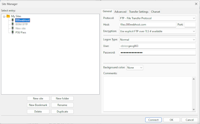
- Double-click on the public_html folder to access the part of your webspace that's open to the world to see (where you'll want to post your projects).
- To transfer a file from your local system to your webspace, navigate to the file in the left-hand pane, right-click on the file and select Upload. (Or drag and drop from the local site to the remote site.)
- When finished transferring files, you can disconnect from the remote server by clicking on the button with the red X.
To avoid having to enter the same connection parameters every time, you can store them as follows:
- Open the Site Manager (1st button on toolbar).
- Click New Site.
- Give a name to your connection (e.g., PSU web space).
- Enter the Host and Port values as specified above.
- Set the Protocol to FTP - File Transfer Protocol.
- Set the Logon Type to Normal or Ask for password (depending on whether you allowed FileZilla to store your password or not).
- Set the User to your website name (again probably surnamegeog863).
- Click Connect and enter your password if prompted.
Going forward, you can connect to your webspace in FileZilla by going to the Site Manager dialog, selecting the connection you created above, and clicking Connect.
Note: The application is set up by default to show a directory tree and a file listing for both the local and remote sites. If you're like me and prefer to see the directory tree and files in a single pane, you can toggle the directory trees off by clicking on the 3rd and 4th buttons in the toolbar.
Connect using the 000webhost File Manager
- This is a web-based means of uploading files to your web space.
- If you check out the Dashboard (click "Manage") then you'll see a few icons - try File Manager and it'll show you your folders - public_html is where you'll be putting your html, js and css files later in the class. A bit like Windows Explorer or Finder on a Mac you can click on the folder names on the left and create new folders with the icons in the top right. I'd suggest a folder per lesson to keep everything neat and tidy.
- Going this route doesn't require installing any additional software and the interface is fairly self-explanatory. The downside is that the interface is a bit clunky and tedious.
You may encounter some web publishing tutorials that recommend you set up a blog. Blogs are preferable to a plain personal web page for most students because blogging software provides page authoring tools that simplify the publishing process. However, for this course, you should avoid setting up a blog. You will need to be able to write your own HTML from scratch and the blogging tools will only complicate matters.
Video Recording with ScreenPal
Video Recording with ScreenPal (formerly Screencast-O-Matic)
Some assignments in this course will require you to use screen recording software to record and then share videos with your instructor and peers. We recommend using ScreenPal (which used to be called Screencast-O-Matic) because it is free and easy to use. If you are not familiar with it, please take some time to learn how to use it during orientation week. The first assignment that uses ScreenPal is in Lesson 1. The details will be provided within the lesson. The more comfortable you are with ScreenPal, the more effective your video will be and the better your grade will be. There are a couple of considerations to be aware of about ScreenPal .
- You will need to set up an account on screenpal.com to be able to share links to your videos. Do not use your Penn State userid and password for this. You can sign up with a Google account or using an email address.
- When it is time to create your video to share, keep in mind that there is a 5-minute time limit for your assignments so you need to plan what you want to record ahead of time. ScreenPal has a 15-minute time limit, so be sure to keep track of your time.
- You may want to practice what you plan to say and time it to make sure that you won’t go over the time limit. Talking while demonstrating a piece of software takes a certain skill, so if this isn’t something that you are familiar with, practice that too. Don’t be discouraged if you have to re-record your video. Since they are only 5 minutes long, it is not a huge time commitment and it is to be expected with anything new.
- Help videos are available to teach you how to use the tool on the ScreenPal Help page. Be sure to review the videos before you try to create your first video.
To Make your Video
- Go to the ScreenPal (SP) website. You can watch a quick demo before you get started. You should use the FREE service, which is linked at the bottom of the home page. You may choose to use another screen capture software program if you prefer. You should just make sure that you can save your finished file as an MP4 for submission for this course.
- Second, record your screen while you give your five-minute demonstration (make sure the audio is clear - using a headset microphone is normally the best way to ensure decent audio quality).
- Third, save it as a video file when you are done recording. You should save it as an MP4, and give it an appropriate, descriptive filename. Then click the green Publish button.
To Share Your Video
- Allow ample time for the video to show up in the My Uploads section of the Your Account page.
- Watch the Hosting video tutorial on the Help page to learn how to get the URL for your video to share with your instructor and peers.