Lesson 5: Introduction to Arc GIS Pro and 3D Modeling ArcGIS Pro
Overview
Overview
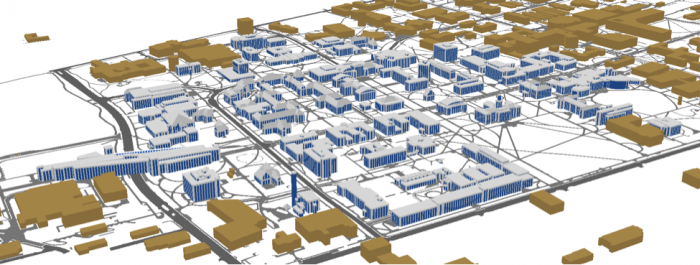
In this module, you will build a 2D map of the University Park campus including buildings, trees, roads, walkways, and a digital elevation model (DEM). You will learn how to convert 2D maps to 3D presentations. Then procedural symbology that we have created for you in CityEngine will be imported and applied to the 3D map to create a realistic scene.
Learning Outcomes
By the end of this lesson, you should be able to:
- Explain options for 3D modeling within Arc GIS Pro
- Understand ArcGIS Pro's integrated 2D–3D environment (Local and Global Scenes)
- Convert a 2D map to a 3D scene
- Explain 3D symbology
- Extrude features to 3D symbology
- Find an example of a 3D CityEngine/ArcGIS Pro model: campus model
- Compare procedural modeling rules (.cga) vs procedural rule package (*.rpk)
- Create a 3D model of elevation (DEM)
- Create a 3D scene from a 2D building footprints of campus-based on the DEM
- Employ a procedural rule symbology based on the rule package
- Link procedural rule symbology to attributes table
- Distinguish static modeling from procedural modeling
- Restructure the map and represent the 3D scene based on the imported model
Lesson Roadmap
| To Read |
|
|---|---|
| To Do |
|
Questions?
If you have any questions, please post them to our "General and Technical Questions" discussion (not e-mail). I will check that discussion forum daily to respond. While you are there, feel free to post your own responses if you, too, are able to help out a classmate.
Section One: Create a Map of University Park Campus
Section One: Create a Map of University Park Campus
Introduction
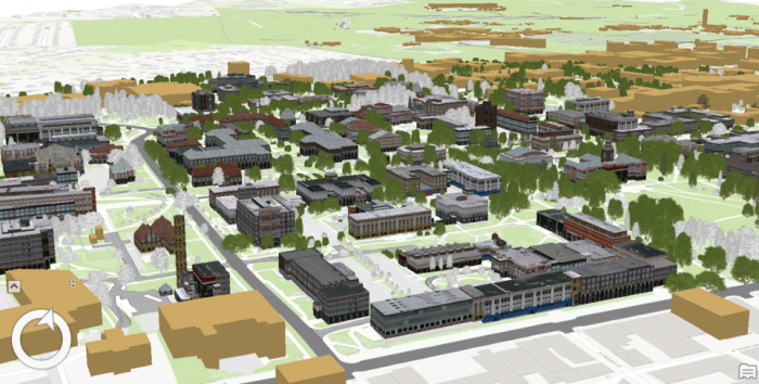
The first step into 3D modeling using ArcGIS Pro is making a map. First, you will create a project. Then you will add necessary data to your map where you have all the tools you need. Then, you will explore the University Park Campus with navigation tools and bookmarks. This 3D model of the University Park Campus will be the final result of this lesson.
1.1 Start a Project
1.1 Start a Project
If you do not have ArcGIS pro installed on your computer, please install it before continuing.
The first step in making a map is creating a project, which contains maps, databases, and directories.
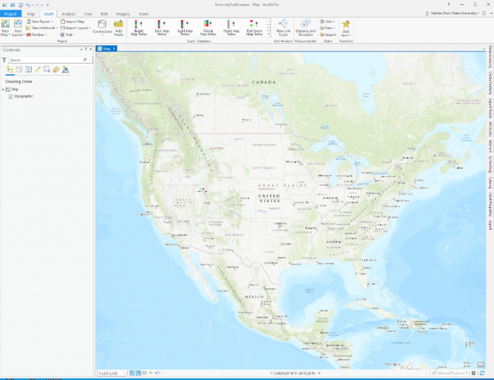
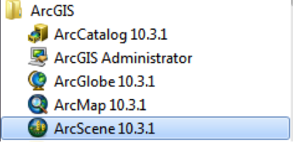
- Start ArcGIS Pro 2.7
 Credit: 2021, ArcGIS [2]
 - Sign in using your licensed ArcGIS account. See this link [3] for how to sign in using the Penn State account.
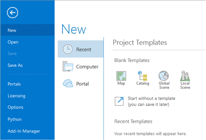
- When ArcGIS Pro opens, you can see a list of project templates under the heading “Create a New Project”. If you have created projects before, you can also see a list of your recent projects.
Project templates are useful in creating a new project because they have aspects of ArcGIS Pro that are important including folder connections, access to databases and servers, and predefined maps.
A Blank template starts a new empty project. It means you won’t have the aspects mentioned above and will start from scratch to build your project. Scene views are for 3D map presentations. Global Scene is a useful template when your data is best represented on a globe. A Global Scene creates a project based on ArcGlobe (part of 3D Analyst extinction of ArcGIS for Desktop). Local Scene is useful for a small area to perform analysis or edit. It is similar to ArcScene in ArcGIS for Desktop. The Map template is suitable for creating a 2D map for your project. It creates a geodatabase in the project folder.[1]
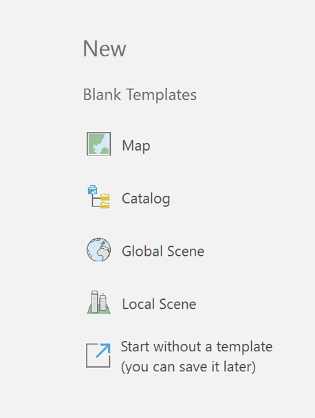
- Click on Map under ‘New’. The Map template is suitable for creating a 2D map for your project. Other templates are for 3D maps. Selecting Map.aptx will let a new window appear: Create a New Project.
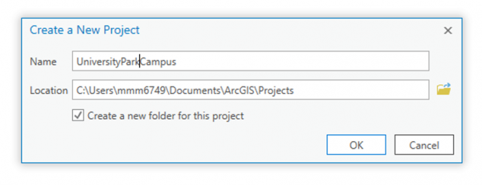
- Name the project “UniversityParkCampus”. By default, the project will be saved to the C: Drive where the ArcGIS folder is located. Change the location if desired.
 Credit: 2021, ArcGIS [2]
 - Click OK. The project opens and displays a map view.
 Credit: 2021, ArcGIS [2]
[1] For more information on project templates: (1) ArcGIS Pro [4], (2) GISP, Tripp Corbin. 2015. Learning ArcGIS Pro. Community Experience Distilled. Packt Publishing: P. Accessed September 22, 2016. http://lib.myilibrary.com?id=878863 [5].
1.2 Add Data to the Map
1.2 Add Data to the Map
To explore Penn State’s University Park Campus, you need data. Download the data [6]. You can save the data package on any location on your computer. Please make sure to unzip the file. It is highly recommended that you save data in the project folder you created before, UniversityParkCampus. The reason is that if you have to move to a different computer, saving everything in your project folder will avoid (most likely) issues with connecting data to your project.
Note: ESRI ArcGIS software is sensitive to the change of data location. If the location address is changed compared to where the addresses are stored in the project, you have to re-link data.
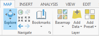
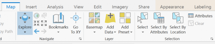
- Go back to the ArcGIS Pro project. At the top of the page, a ribbon is located. Click on the map tab. In the layer group, click on Add Data.
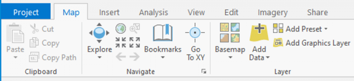 Credit: 2021, ArcGIS [2]
The Add Data Window will open. You will have three options for finding data: (1) the project folder, (2) portal (online), and (3) my computer.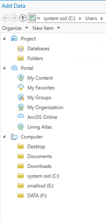 Credit: 2021, ArcGIS [2]
 -
In the pane of the window, under my computer click on the folder that you have saved the data files in. If you have used the default location for saving the project (C:\Users\Yourname\Documents\ArcGIS\Projects), the geodatabase is inside the UniversityParkCampus folder.
-
Go inside the geodatabase and Double-click the following layers to add them to the map: UP_BUILDINGS,UP_Major_Roads, UP_Minor_Roads, UP_Sidewalks, and UP_TREES.
Attention: if you go to the project folder you can see that a geodatabase named exactly as your project has been created: “UniversityParkCampus.gdb’.This is the geodatabase that you will use for saving the results of the analysis. The geodatabase that we have given you (Lesson5.gdb) contains external data prepared for you to start.
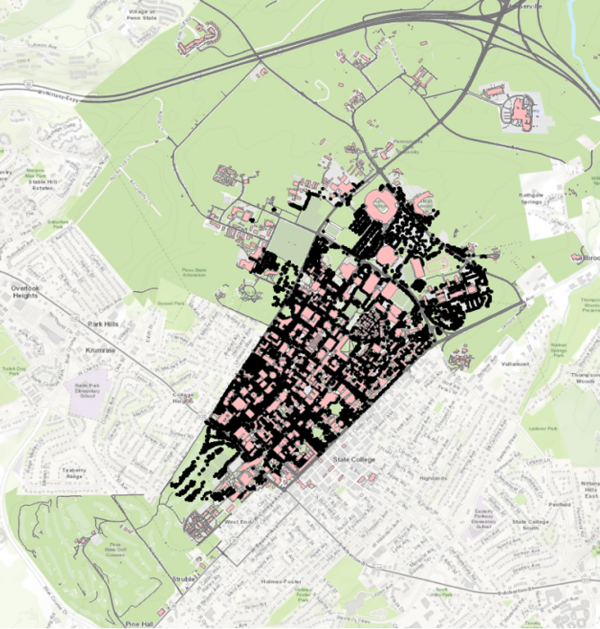 Credit: ChoroPhronesis Lab [1]
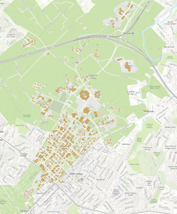
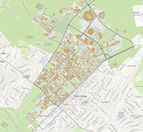
The map will center on the University Park campus in State College, PA.
1.3 Navigate the Map and Create Bookmarks
1.3 Navigate the Map and Create Bookmarks
Before we focus on symbolizing the layers and improve the map, you will learn how to navigate the map and create bookmarks to quickly return to key areas.
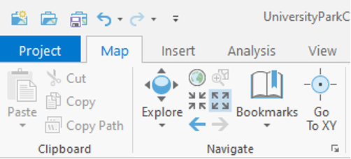
- On the top of the page, a ribbon is located. On the Map tab, in the Navigate group, click the ‘Fixed Zoom Out’ button. The map zooms out a fixed distance.
You can also zoom by positioning your mouse pointer in the map window and using the mouse’s scroll wheel.
 Credit: 2021, ArcGIS [2]
 - Zoom out until you see the entire campus area.
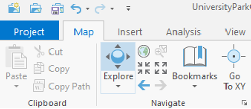
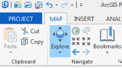
- In the map tab, in the Navigate group, click the Explore button.
 Credit: 2021, ArcGIS [2]
 - Click and drag the map to pan to the west side of campus where the IST (Information Sciences and Technology) building is located.
 Credit: ChoroPhronesis Lab [1]
 - Pan back to the center of the University Park campus.
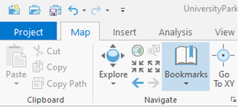
Now, you will create bookmarks to quickly and efficiently navigate to points of interest. - In the Map tab, in the Navigate group, click the bookmarks button and choose a new Bookmark.
 Credit: 2021, ArcGIS [2]
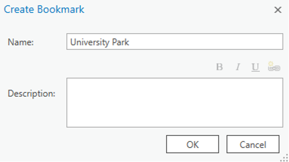
 - Type University Park for the Bookmark Name. Click OK.
 Credit: 2021, ArcGIS [2]
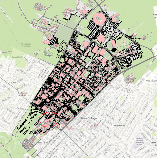 Credit: ChoroPhronesis Lab [1]
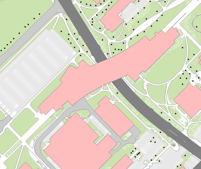
 - Zoom back to the IST building highlighted below. To zoom to a specific extent, press and hold the Shift key and draw a box around the area on the map.
 Credit: ChoroPhronesis Lab [1]
 - Bookmark the IST building. Name the bookmark IST.
- Click the Bookmarks button and click the University Park bookmark.
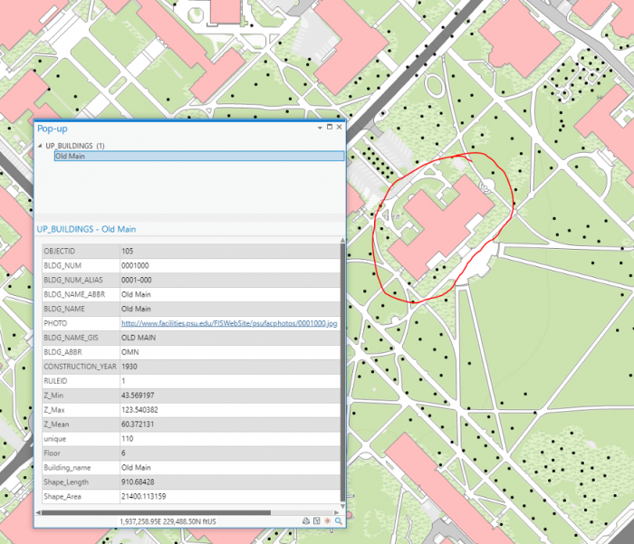
- Click on the building pictured below to open a pop-up window with additional information.
Every feature has a pop-up window. By default, a pop-up displays the attribute data of the selected feature. The above example includes the building’s name and its construction year.
 Credit: ChoroPhronesis Lab [1]
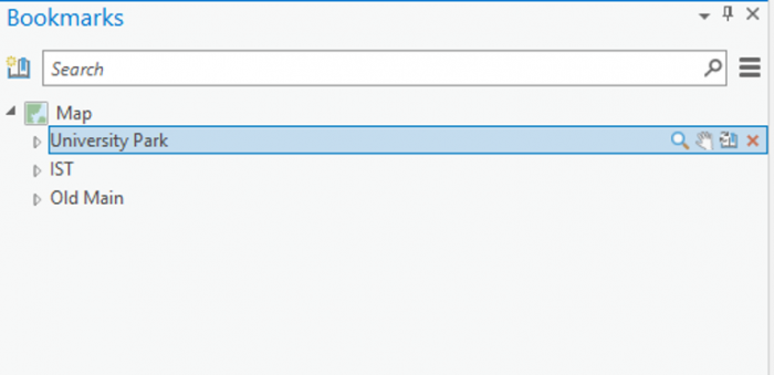
 - Bookmark this building and name it Old Main. You can also access the Bookmarks pane on the right side of your map to get an overview of the bookmarks you created.
 Credit: 2021, ArcGIS [2]
 - Click some of the buildings to learn about the data. You can find the Geography Department and the Hub and bookmark them for practice.
- Return to the University Park bookmark. In the Quick Access Toolbar at the top corner of the ribbon, click the Save button to save your project.
 Credit: 2021, ArcGIS [2]
In the next lesson, you will learn about data symbolization and editing.
Section Two: Symbolize Layers and Edit Features
Section Two: Symbolize Layers and Edit Features
Introduction
You probably noticed during your map-exploration that it was hard to distinguish some of the features because of how they were symbolized. In this section, you will symbolize your map, for example, to enhance readability.
2.1 Symbolize the UP_BUILDINGS layer
2.1 Symbolize the UP_BUILDINGS layer
First, you'll give the buildings layer a more appropriate color.
- If necessary, open the UniversityParkCampus project in ArcGIS Pro.
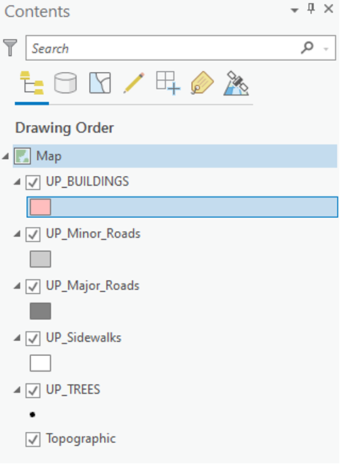
- On the contents pane, uncheck all layers but UP_BUILDINGS. Click the colored rectangle symbol under the UP_BUILDINGS layer.
The Symbology pane opens to the Gallery.
 Credit: 2021, ArcGIS [2]
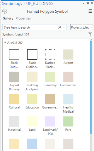 Enter caption hereCredit 2021, ArcGIS
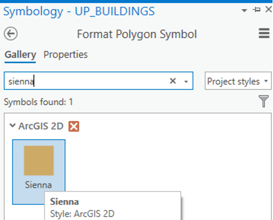
 - In the search box, type sienna and press Enter.
 Credit: 2021, ArcGIS [2]
 - The result is that the symbology for buildings will change to orange-brown. Feel free to explore further color options.
 Credit: ChoroPhronesis Lab [1]
2.2 Symbolize the UP_Major_Roads and UP_Minor_Roads layers
2.2 Symbolize the UP_Major_Roads and UP_Minor_Roads layers
Next, you will change the major roads symbol.
- On the Contents pane, turn on the UP_Major_Roads layer. Click the colored rectangle symbol under the UP_Major_Roads.
- On the Symbology pane, click Properties.
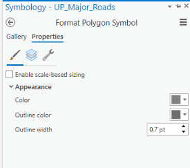 Credit: 2021, ArcGIS [2]
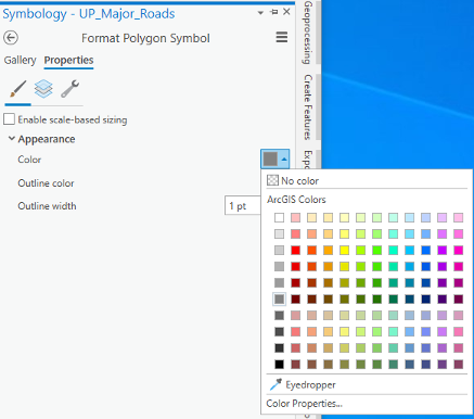
 - Under Appearance, click the drop-down arrow next to Color and choose Gray 50%. For the outline color, choose no color.
Hover over a color to see its name.
 Credit: 2021, ArcGIS [2]
 - At the bottom of the Symbology pane, click Apply.
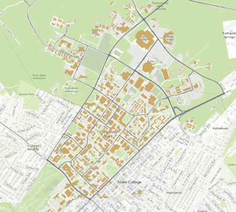 Credit: ChoroPhronesis Lab [1]
Repeat the previous steps for UP_Minor_Roads. Change Minor roads’ symbol to ‘Gray 40%’ with no outline color.
2.3 Symbolize the UP_Sidewalks
2.3 Symbolize the UP_Sidewalks
Next, you will change the UP_Sidewalks.
- On the Contents pane, turn on the UP_Sidewalks. Click the colored rectangle symbol under the UP_Sidewalks.
- On the Symbology pane, click Properties.
 Credit 2021, ArcGIS
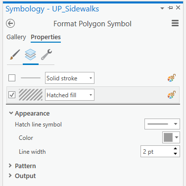
 - Under Appearance, click the drop-down arrow next to Color and choose Gray 40%. For the outline color, choose no color.
- Then click on the Layers tab. Un-check the first option, which is for outline style. Click on the second option and choose hatched fill.
For the hatch line symbol, choose simple stroke (2.0 pt). Hover over to see its name.
Choose 2.5 pt for the line width.
- At the bottom of the Symbology pane, click Apply.
 Credit: ChoroPhronesis Lab [1]
2.4 Symbolize UP_TREES
2.4 Symbolize UP_TREES
Trees in Up_Trees are point features. Here we will show you how to symbolize point features based on attributes. Before symbolizing this layer, explore the attribute table for this layer.
- On the Contents pane, turn on UP_TREES. Right-click the UP_TREES layer and click on the Attribute Table.
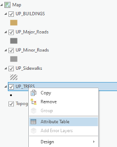 Credit: 2021, ArcGIS [2]
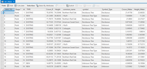
 - Examine the fields in the attribute table.
This tree layer is extracted from LiDAR Imagery collected in 2015. Some of the trees species are existing trees from a 2005 survey. Some have been added to the database as new trees and some are best guesses based on the LiDAR data. Therefore, tree type, listed as ‘symbol’ is only available for some but not all trees. A new tree database is under development for a complete tree database. You can see different tree symbols, such as deciduous and evergreen. You will symbolize the tree layer based on the symbol field.
 Credit: 2021, ArcGIS [2]
 - Close the attribute table.
- Click the point under UP_TREES. The Symbology pane will appear on the left side.
- At the top of the page, a ribbon is located. Click on the appearance tab.
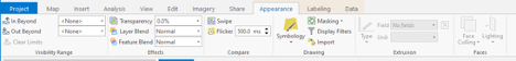 Credit: 2021, ArcGIS [2]
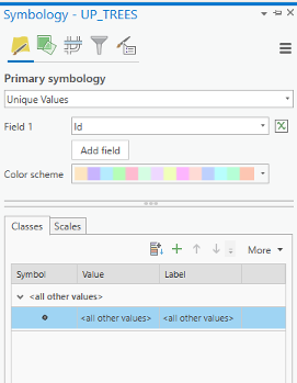
 - Click the drop-down arrow under Symbology and select ‘Unique Values’ under ‘Symbolize your layer via categories’. Now you can see that the symbology pane on the left side has changed to unique values.
 Credit: 2021, ArcGIS [2]
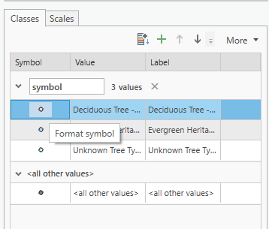
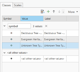
 - Change the value field from Id to symbol. Now you can see different values under symbol attribute.
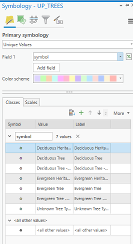
There are three types of deciduous and three types of evergreen and one ‘Unknown Tree Type’ value. Null values belongs to new trees which do not have tree symbol assigned to them. We would like to group all deciduous trees together and all evergreen trees together.
 Credit: 2021, ArcGIS [2]
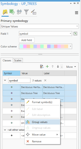
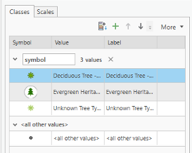
 - Select all three categories for deciduous trees and group them. Do the same for evergreens.
 Credit: 2021, ArcGIS [2]
 - Click on the label values (last column) and change the values to Deciduous, Evergreen, and Unknown, respectively.
- Now select Format symbol for deciduous category.
 Credit: 2021, ArcGIS [2]
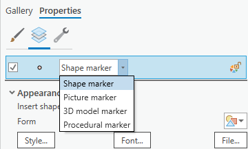
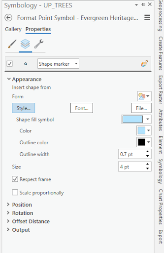
 - For the evergreen symbol, under Layers, choose shape maker from the menu. This time instead of Font, click on Style tab.
 Credit: 2021, ArcGIS [2]
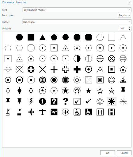 Credit: 2021, ArcGIS [2]For color, choose Tarragon green, and for the outline color black. The outline width should be 0.2 opt and the symbol size, 13 pt.
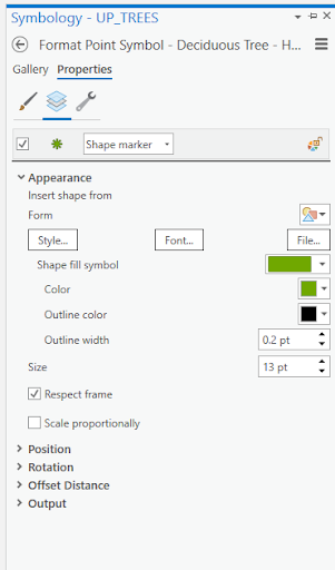 Credit: 2021, ArcGIS [2]
 -
For the evergreen symbol, under Layers, choose shape maker from the menu. This time instead of Font, click on the Style tab.
 Credit: 2021, ArcGIS [2]
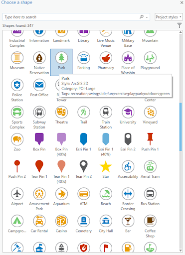 Credit: 2021, ArcGIS [2]
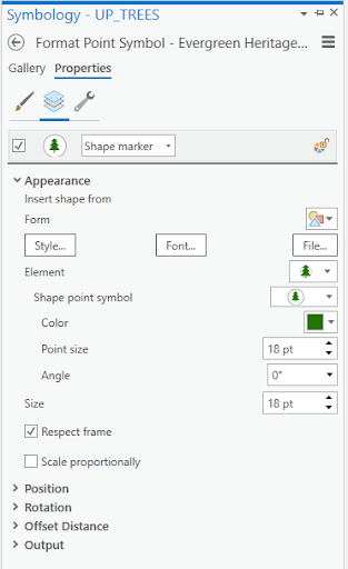
Based on the screenshot, choose Fir Green for the color, and 18 pt for the symbol size.
 Credit: 2021, ArcGIS [2]
 -
For the unknown symbol, under Layers, choose shape maker from the menu.
Then click Font and choose shape 107 and click ok.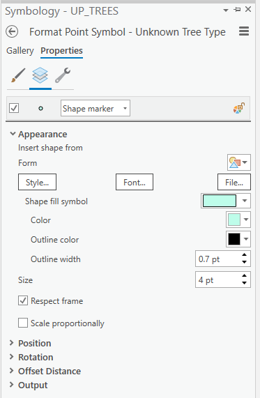 Credit: 2021, ArcGIS [2]Based on the screenshot, choose Medium Olivenite for the color, no color for the outline color and 0.01 pt for the outline width, and finally 13 pt for the symbol size.
 Credit: 2021, ArcGIS [2]Click apply on the bottom of the pane.
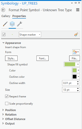 Credit: 2021, ArcGIS [2]
To make the trees more visible, you can drag the layer on top of the layers in Content pane. The final result would be like the following image: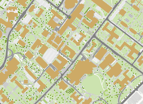 Credit: ChoroPhronesis Lab [1]
 - Make a Screenshot of UP Campus with all symbolized layers for your graded assignment. This is labeled Task 1 on the Tasks and Deliverables.
Section Three: Explore Raster Data
Section Three: Explore Raster Data
Introduction
To present a 3D scene of University Park Campus, you need an elevation base for your building footprints and other layers such as roads and trees. In this section, we focus on preparing the Digital Elevation Model (DEM) for University Park Campus. The Digital Elevation Model (DEM) is a bare earth elevation model. It has been extracted from LiDAR data.
3.1 Add and Explore Raster Data
3.1 Add and Explore Raster Data
In the previous section, you worked with feature data, data displayed as discrete objects, or features. While feature data is great for depicting buildings, roads, or trees, it is not the best way to depict elevation over a continuous surface. To do that, you'll use raster data, which can demonstrate a continuous surface. Raster data is composed of pixels, each with its own value. Although it looks different from feature data, you add it to the map in the same way.
- If necessary, open the University Park Campus project in ArcGIS Pro.
- In the Map tab, in the Layer group, click the Add Data button.
- In the Add Data window, under My Computer, navigate to where you have saved the data. Double-click UP_BareEarth to add it to the map.
- In the Contents pane, uncheck the boxes next to all layers, leaving only UP_BareEarth, UP_Buildings, and the basemap visible.
The elevation unit is feet. Unlike the feature layer, which has shape geometry, raster layer use pixel matrices in which each pixel stores its own value. The layer resolution, the size of its pixels or cell size (x,y) is 2 by 2 square feet. The result, 4, means that each pixel represents an area of four square feet.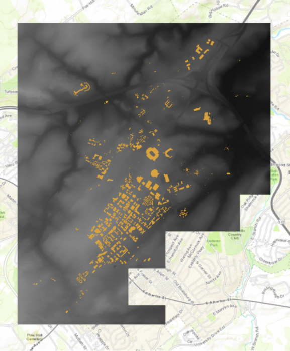 Credit: ChoroPhronesis Lab [1]
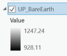
 - In the Contents pane, click the arrow next to UP_BareEarth to view its symbology.
Instead of a single symbol, this layer has a color scheme for different values. The values represent elevation in feet. The elevation ranges from about 825 feet above sea level (black) to about eighteen hundred feet above sea level (white).
 Credit: 2020 ArcGIS [2]
 - On the Map tab, in the Navigate group, click Explore. Click anywhere on the raster to open a pop-up window.
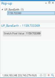 Credit: 2021, ArcGIS [2]
The pop-up shows the Pixel Value, which indicates the actual value of a pixel. In this raster, it shows the elevation. In the above image, the selected pixel has an elevation of about 1159 feet above sea level.
- Close the pop-up.
3.2 Smoothing the DEM and Creating Contours
3.2 Smoothing the DEM and Creating Contours
Before exploring the raster data in 3D, we need to smooth the elevation model, so the 3D model of campus fits the elevation model nicely. In order to monitor the level of smoothness of a DEM, creating contours can be helpful. A contour set built based on a raw digital elevation model (DEM) data can show minor variations and irregularities in the data. Creating a smooth contour set for topography is helpful in smoothing the data.
Note: the smooth grid should not be used for any analysis that requires raw DEM. For instance, building height cannot be extracted from a smoothed DEM.
- At the top of the page, a ribbon is located. Click on the analysis tab.
 Credit: 2021, ArcGIS [2]
 - In the Geoprocessing group, click Tools.
- In the Geoprocessing pane, search ‘Focal Statistics’.
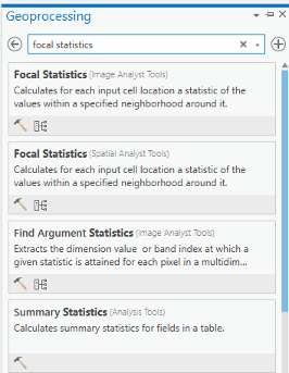 Credit: 2021, ArcGIS [2]
 - Select the Focal Statistics, which is located under Spatial Analyst Tool.
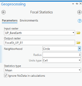
The Focal Statistics tool will resample from the DEM and apply a search distance defined by cells or model distance.
- Choose UP_BareEarth as the input raster. Name the output raster so you can remember it! Every smoothed grid should be named and documented with information describing the smoothing process. The default name is FocalST_UP_B1. It means focal statistics phase 1.
- Select Circle from the drop-down next to Neighborhood and set the smoothing Radius to 3. Leave all other default settings. Specify MEAN as the Statistics type.
 Credit: 2021, ArcGIS
 - Click Run on the bottom of the pane to create the first smoothed grid.
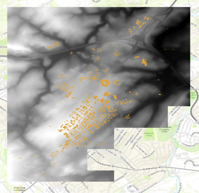 Credit: ChoroPhronesis Lab [1]
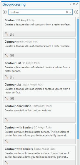
 - Contour lines can be created from this smoothed grid. Go back to the search bar in the Geoprocessing pane and search contour. Select contour with Barriers (Spatial Analyst Tool).
 Credit: 2021, ArcGIS [2]
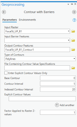
 - Select FocalSt_UP_B1 as the Input raster and specify the output contour feature as FocalSt_UP_B1_Contour1. Types of Contour will be polyline. Set the Contour Interval to 5 feet and Indexed Contour Interval to 20 feet. Leave default values for other options. Click Run to create the contours.
 Credit: 2021, ArcGIS [2]
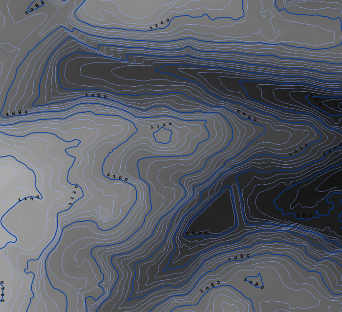
 - When the contours have been drawn, zoom in and inspect them. Notice that these lines are quite dense, especially when the entire model is viewed. Open the attribute table and verify that approximately 2,310 contour lines were created. These contours range in elevation from
930 to 1245 feet.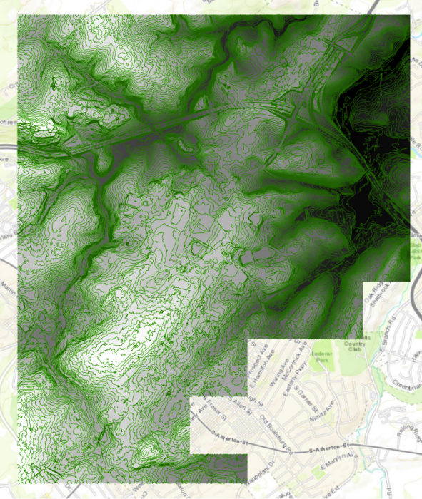 Credit: ChoroPhronesis Lab [1]
 - We can symbolize the indexed contour to have a better sense of elevation. Click the contour layer in the contents pane. Click the appearance tab. Under Symbology, select unique values. On the Symbology Pane symbolize based on value field “Type”. Type 1 are contours, which are every 5 feet and type 2 are barriers, which are every 10 feet.
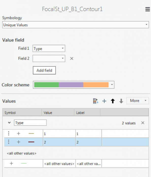 Credit: 2016 ArcGIS [2]
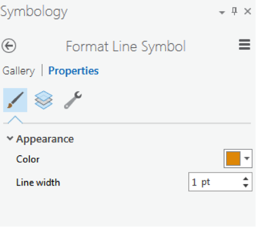
 - As you learned in the previous section, select symbology for each type. When you click format symbol, you can either choose Gallery (choose from preexisting styles) or choose Properties. We suggest properties.
 2016 ArcGIS [2]
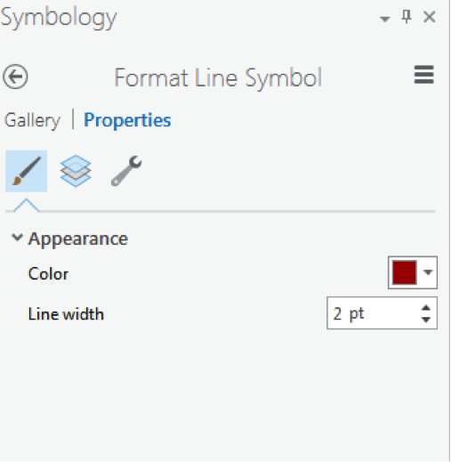 Credit: 2016 ArcGIS [2]
 -
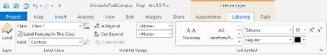
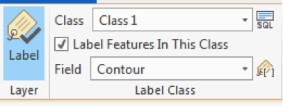
Click the contour layer in the contents pane. Make sure the symbol is highlighted by clicking on it. From the top ribbon, under Feature Layer, click Labeling. Under Label Class group, choose Contour for Field value. For class value click on the SQL button.
 Credit: 2021, ArcGIS [2]
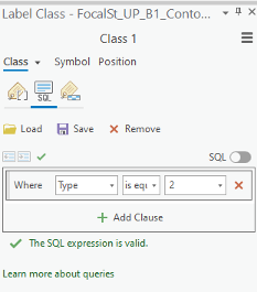
 - In Label Class pane, under SQL, click New Expression. Choose Type is equal to 2. With this selection, you will only label indexed contours. Click Apply.
 Credit: 2021, ArcGIS [2]
 - Go back to the labeling tab on top of your map. Choose font Corbel, size 12, bold, black.
- Click Label button under Layer group.
 Credit: 2016 ArcGIS [2]
 - Your final result should look like this image.
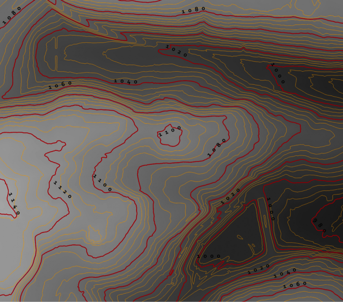 Credit: ChoroPhronesis Lab [1]
 - Keep this contour layer for comparison with the final result.
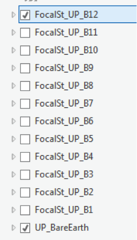
- To have a smoother DEM, you have to repeat step 5 to 7 for a few times (Focal Statistics). Let’s say 12 times. Every time, you have to use the previous smoothed DEM. For instance, for the second round, you will use ‘FocalSt_UP_B1’ as an input. Keep the same naming system and options. Name the second output as FocalSt_UP_B2. You do not need to create contours for every smoothed layer. You will create another contour layer for the last output ‘FocalST_UP_B12’ to compare it with the first result.
 Credit: 2016 ArcGIS [2]
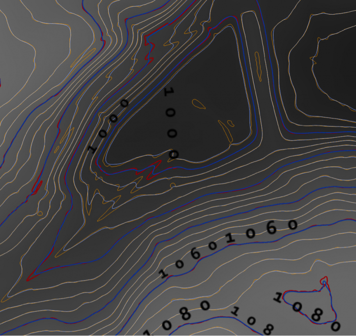
 - Now that you have the final DEM Layer (FocalST_UP_B12), Create Contour with Barriers for it. Repeat step 11 to 15. You can see how much smoother the new contours are. It means that we have a smooth DEM that is easier to work with.
 Credit: ChoroPhronesis Lab [1]
 - By choosing another color for the ‘FocalSt_UP_B1_Contour12’, you can compare the smoothness with the first created contour layer. You can choose light blue for the contours and dark blue for index contour. Repeat the labeling process to label your contours.
 Credit: ChoroPhronesis Lab [1]
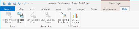
 - Select ‘FocalSt_UP_B1_Contour12’ in the Content Pane. From the top ribbon, choose Data, under Raster Layer. Click Export Data.
 Credit: 2021, ArcGIS [2]
 - As input Raster, choose ‘FocalSt_UP_B12'. Rename the output Raster to Smoothed_DEM. Click Run.
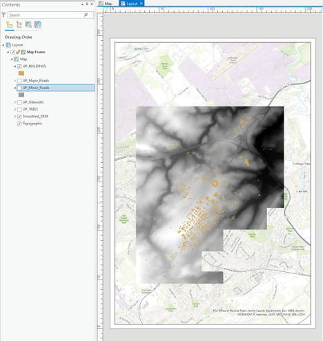
You do not need the other raster/contour layers you created (from B1 to B12). You can remove them from your Contents pane. Also, remove UP_BareEarth. - For your final Assignment, you need a map of Smoothed_DEM and its full extent. Turn off all layers but Smoothed_DEM and Topographic. Zoom in or out, so that the DEM is in the center of your map.
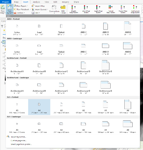
- On top Ribbon, go to the Insert tab and add a new layout of A4 size. a layout page is opened.
 Credit: 2021, ArcGIS
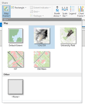
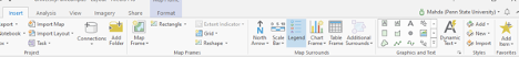
 - On Insert tab, click Map Frame and select the map option with Scale.
 Credit: 2021, ArcGIS
 - Draw the frame on the A4 paper layout that you would like the map to appear.
 Credit: 2021, ArcGIS
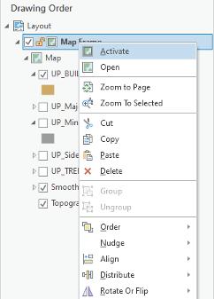
 - Under Layout, right-click on Map Frame and click Activate. You can zoom in and out until get the desired scale. Also, on the bottom of the page you can enter the desired scale. When finished, click Layout on top ribbon and Close Activation.
 Credit: 2021, ArcGIS [2]
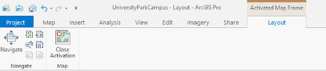 Credit: 2021, ArcGIS [2]
 - Under insert, click Legend on Map Surrounds.
 Credit: 2021, ArcGIS [2]
 - Draw the legend wherever you like on the Layout area. You can try to add a north arrow or scale bar if you are interested.
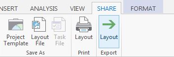
- Click the Share tab. Under Print click Layout. Select Adobe PDF and Print the results. This is labeled as Task 2 on the Tasks and Deliverables.
 Credit: 2016 ArcGIS [2]
Section Four: Explore 3D Data
Section Four: Explore 3D Data
Introduction
In this section, you’ll visualize 3D data. You will learn how to convert a 2D map to 3D scene, visualize the DEM layer and other feature classes such as trees and buildings.
4.1 Convert a Map to a Scene
4.1 Convert a Map to a Scene
Most commonly we display data as a 2D map (although this may change in the future). Traditionally, in ArcGIS software, a 2D map was displayed in ArcMap and a 3D scene displayed by ArcScene.
In ArcGIS Pro, you will have 2D maps and 3D scenes in the same platform. A scene is a map that displays data in 3D. By default, ArcGIS Pro will convert a map to a global scene, which depicts the entire world as a spherical globe. Since your area of interest is University Park Campus, not the entire globe, you will need to change the settings so the map converts to a local scene instead.
- Before starting this section, turn on UP_BUILDINGS and Smoothed_DEM layers.
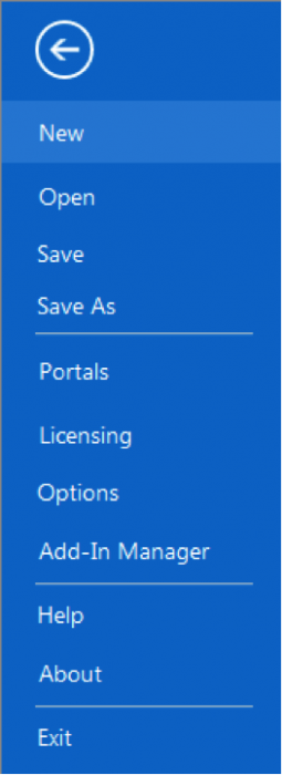
- Click the Project tab.
 Credit: 2016 ArcGIS [2]
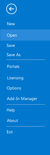
 - Click Options, on the blue pane.
 Credit: 2016 ArcGIS [2]
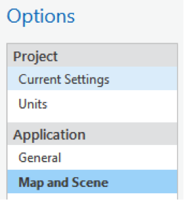
 - The Options window will appear. Under Application, click Map and Scene.
 Credit: 2016 ArcGIS [2]
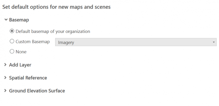
 - Choose the default base map of your organization.
 Credit: 2019 ArcGIS [2]
 - Click OK. In the blue pane, click the back arrow to return to your map.
- On the View tab, in the View Group, click Convert and from the drop-down menu choose ‘To Local Scene’.
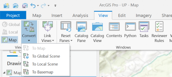 Credit: 2019 ArcGIS [2]
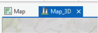
Your map converts to 3D, creating a new pane called Map_3D. You can go back to your 2D map at any time by clicking the Map tab.
 Credit: 2016 ArcGIS [2]
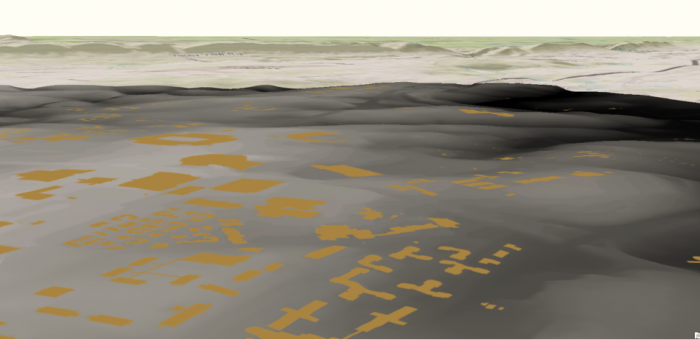
 - Under the Map_3D pane, still, your data is 2D and flat. This is because your layers are designed as 2D. You will change them later in this section. If the UP_BUILDINGS layer is in the 3D Layers, drag it down to 2D Layers.
- In the Map_3D scene, hold down the scroll wheel or the V key and drag the pointer to tilt and rotate the scene. Pan and zoom the same way you would in a 2D map.
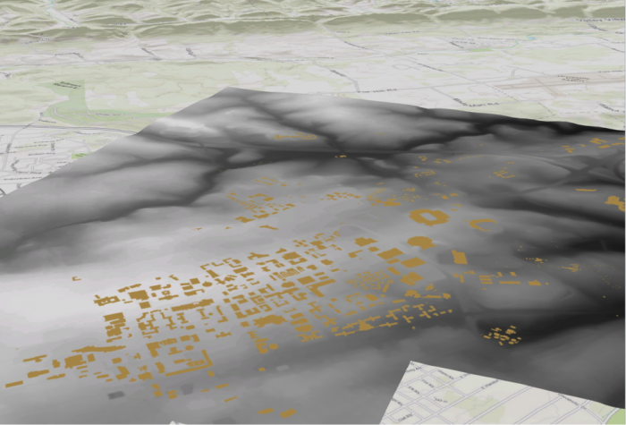 Credit: ChoroPhronesis Lab [1]
The flatness of the campus contrast with hills in the distance. By default, scene uses a map of elevation data, called an elevation surface, to determine the ground's elevation. It is a low resolution but spans the entire world.
- On the Map tab, in the Layer group, click the Add Preset button and choose Ground. The Add elevation source window opens. The Smoothed_DEM should be set as the ground in the area around campus. Navigate to the location of Smoothed_DEM. Click Select.
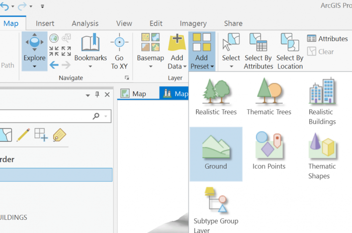 Credit: 2019 ArcGIS [2]
 - Pan, zoom, and tilt to navigate the scene and better view the new ground elevation. You may have to zoom very close to see the shifts in elevation.
 Credit: ChoroPhronesis Lab [7]
4.2 Extrude the UP_BUILDINGS Layer
4.2 Extrude the UP_BUILDINGS Layer
Another layer that is flat but should not be is the building footprint. The UP_BUILDINGS layer has height data in its attributes. It has been extracted from LiDAR data (as discussed in Lesson 4). To display the layer in 3D, you will use a command called extrusion, which displays features in 3D by using a constant or an attribute as the z-value. In this layer, the attribute will be Z_Mean.
- In the Contents pane, click and drag the UP_Buildings layer from the 2D Layers group to the 3D Layers group.
- Right-click on UP_BUILDINGS layer and select properties.
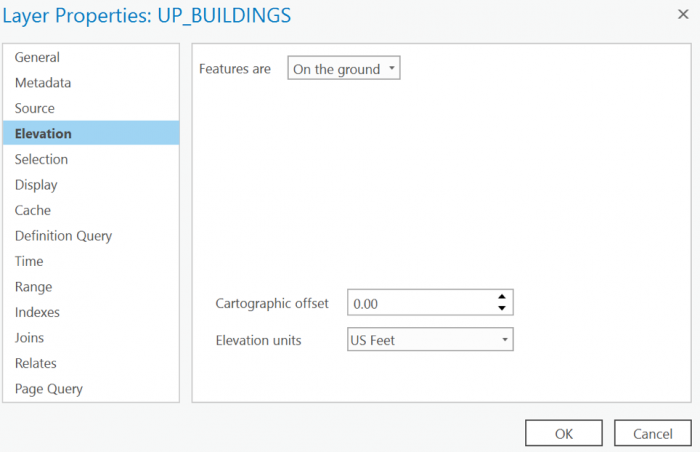
- Go to Elevation tab. Select the drop-down menu in front of ‘Features are’.
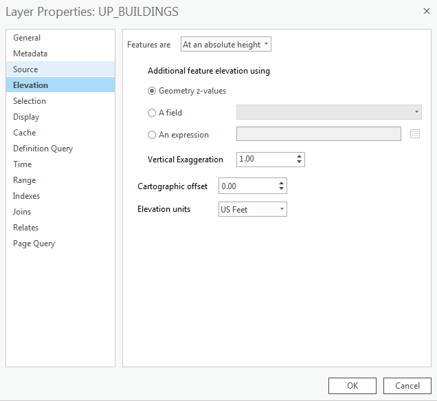 Credit: 2016 ArcGIS [2]
 - Select ‘On the ground’ option. This means that the buildings layer uses the DEM as the ground base for elevation. For ‘Elevation units’ choose US feet. Click OK.
 Credit: 2019 ArcGIS [2]
 - In the Contents pane, right-click UP_BUILDINGS and choose Attribute Table. Find the Z_Mean field. You will extrude the layer with values in this field.
- Close the attribute table.
- Make sure the UP_BUILDINGS is selected on the Contents pane.
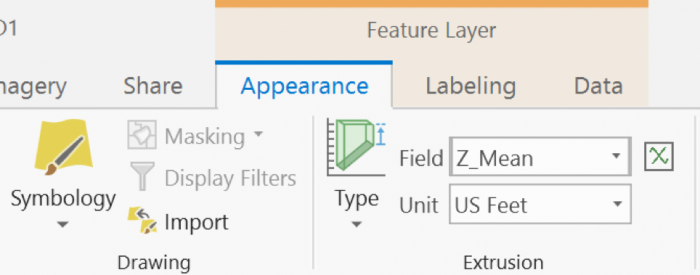
- On the Appearance tab, in the Extrusion group, click the Type button and choose Max Height
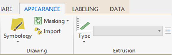 Credit: 2016 ArcGIS [2]
 - Click the menu next to Type and choose Z_Mean.
The features are extruded, meaning they are given a height value based on the selected field. They now appear 3D on the map.
 Credit: 2019 ArcGIS [2]
 - Turn off Smoothed_DEM Layer. Now, you can see the extruded buildings on top of the base map.
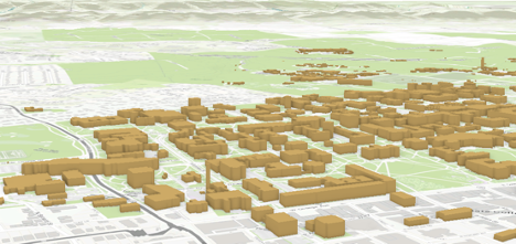 Credit: ChoroPhronesis Lab [1]
 -
Now you can turn on Roads and sidewalks. Make sure they are under 2D layers. Later in this Lesson, you will extrude trees and symbolize them.
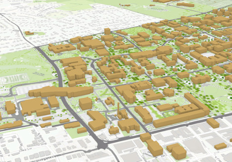 Credit: ChoroPhronesis Lab [1]
 - If you turn off the basemap (Topography), you will have a better view of the roads and sidewalks.
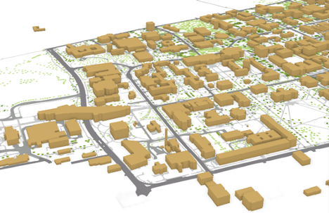 Credit: ChoroPhronesis Lab [1]
 - Save the Project.
Section Five: Display a Scene with More Realistic Details
Section Five: Display a Scene with More Realistic Details
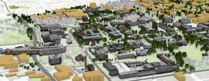
Introduction
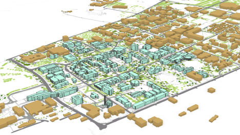
As you can see, the extruded buildings in the previous section, are blocks with no details, just the elevation. In this section, you will learn how to present part of west campus with more details. To do so, you should remove some of the features from UP_BUILDINGS that overlap with the layer that has more detailed information. This new layer (UP_Roof_Segments), that you will add to the map, consists of roof segments with detailed elevation. This information has been extracted from LiDAR data. In other words, instead of treating buildings as a big, undifferentiated chunk, every change in shape or elevation in each building has been detected and a new layer that represents those change/segments have been created. In Module 4, we have explained the process of creating this layer in detail.
5.1 Add and Extrude the UP_Roof_Segments
5.1 Add and Extrude the UP_Roof_Segments
In this section, you will remove the overlapping part of UP_BUILDINGS Layer with the P_Roof_Segment. This means that the UP_Roof_Segments represents part of campus with more details while UP_BUILDINGS will represent the rest of the campus (where the detailed model is not available) with less detail.
Therefore, you should remove the overlapping feature from UP_BUILDINGS Layer. This means that the UP_Roof_Segments represents part of campus with more details while UP_BUILDINGS will represent the rest of the campus (where the detailed model is not available) with less detail.
- On the contents pane, uncheck UP_BUILDINGS Layer.
- On the Map tab, in the Layer group, click the Add Data button.
 Credit: 2016, ArcGIS [2]
 - Add UP_Roof_Segments from the geodatabase (Module5.gdb) that you downloaded earlier in this Lesson.
- Right-Click on UP_Roof_Segment layer and select properties.
- Go to Elevation tab. Select the drop-down menu in front of ‘Features are’.
- Select ‘On the ground’ option. This means that the buildings layer uses the DEM as the ground base for elevation. Click OK.
- Click UP_Roof_Segment on the contents pane.
- On the Appearance tab, in the Extrusion group, click the Type button and choose Max Height.
 Credit: 2016, ArcGIS [2]
 - Click the menu next to Type and choose Z_Mean_Roof.
- Change the layer outline width to 0.3.
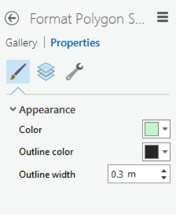 Credit: 2016 ArcGIS [2]
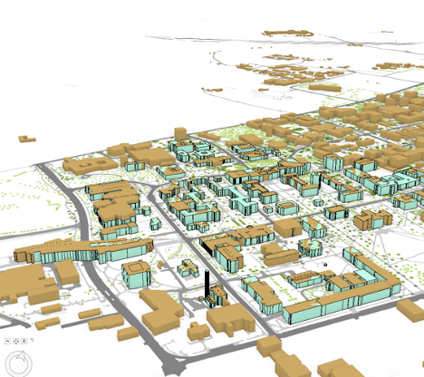
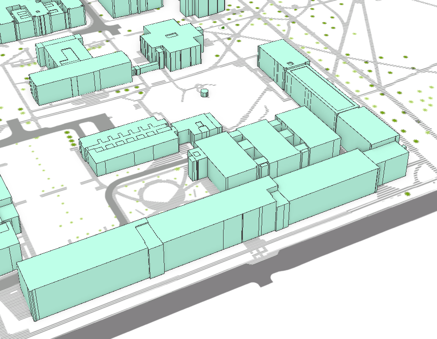
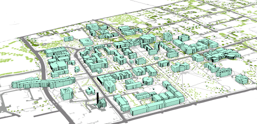 Credit: ChoroPhronesis Lab [1]
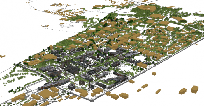
This is how your model should look like. You can navigate by holding down the scroll wheel or the V key and drag the pointer to tilt and rotate the scene. You can see the level of details each building presents in 3D.
 Credit: 2019, ArcGIS [2]
 -
To see how the buildings look like in reality, go to GoogleMaps [8]. Search for University Park Campus.
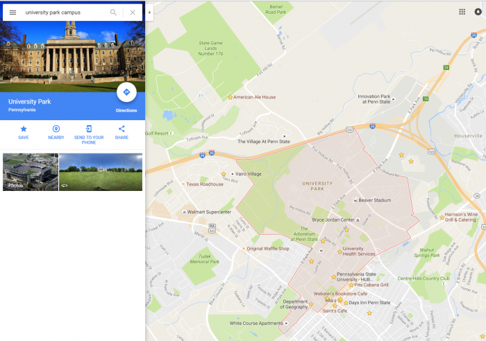 Credit: Google Maps [9]
Click the earth option at the bottom of the page.
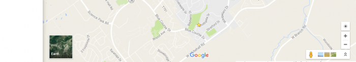 Credit: Google Maps [9]
Your map will turn to Earth view.
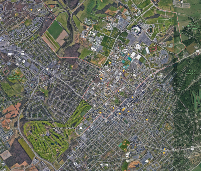 Credit: Google Maps [9]
Zoom in to Penn State Alumni Association. This is how the roofs structures look like:
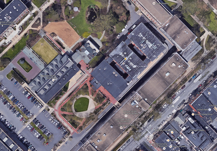 Credit: Google Maps [9]
Go back to your ArcGIS Pro project and find the same building. You can find the same level of detail in roof structure.
 Credit: ChoroPhronesis Lab [1]
Go back to Google map and explore more. You see that some of the buildings have flat roofs and some shed roofs. However, in your 3D model, all the roofs are flat. You will add different roof types later in this module.
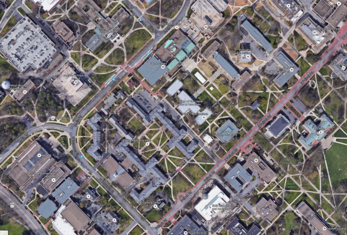 Credit: Google Maps [9]
 - Go back to ArcGIS Pro. In the content pane, turn the UP_BUILDINGS layer back on and make sure that it is located under the UP_Roof_Segments layer. In parts of campus which has both layers, the two layers are not overlapping well; this is because UP_Roof_Segments layer masking UP_BUILDINGS and has more details in the change of elevation than the UP_BUILDINGS Layer.
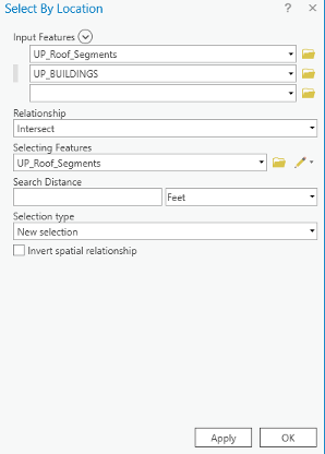
- In order to remove features from UP_BUILDINGS, you should select those features. The best way to do that is to select by location. On the Map tab, in the Layer group, click the ‘Select By Location’ under Selection group.
- You will select features from UP_BUILDINGS that intersect with UP_Roof_Segments. Therefore, choose the factors as shown in the image below. Click Run.
- If you uncheck the UP_Roof_Segments layer, you can see the part of UP_BUILDINGS that has been selected. This is the part that overlaps the UP_Roof_Segments.
 Credit: ChoroPhronesis Lab [1]
However, what you need to keep is the rest of the buildings, not what has been selected. Therefore, you will switch selection to select the remaining part of the campus.
- Right-click on Up_BUILDINGS. Under Selection, choose Switch Selection.
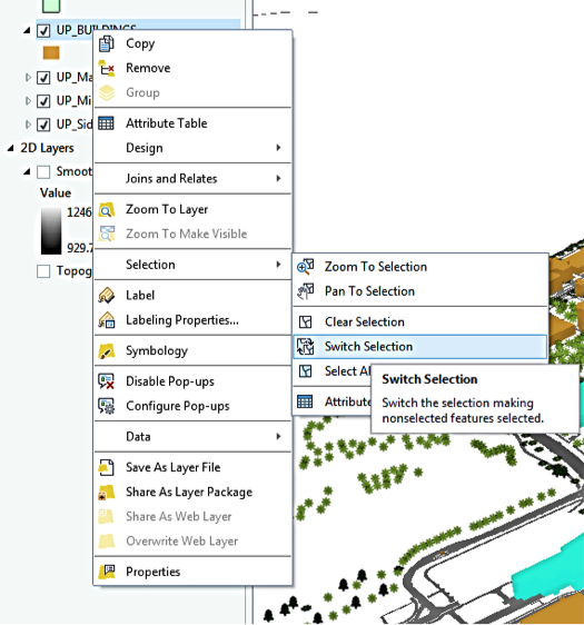 Credit: ChoroPhronesis Lab [1]
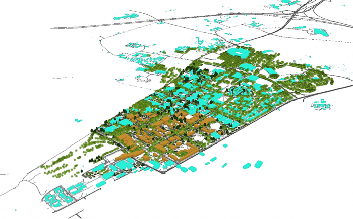 Credit: ChoroPhronesis Lab [1]
 - Now, you will export the selected features. Right-click on UP_BUILDINGS layer and click Data, choose Export Features.
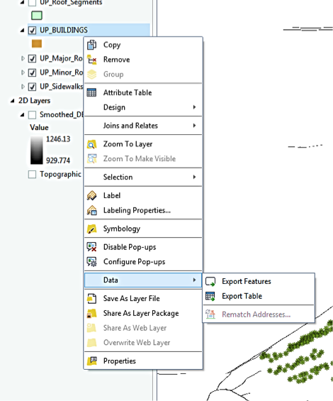 Credit: 2016 ArcGIS [2]
 - Rename the output features to ‘Building_Footprints’. And click Run.
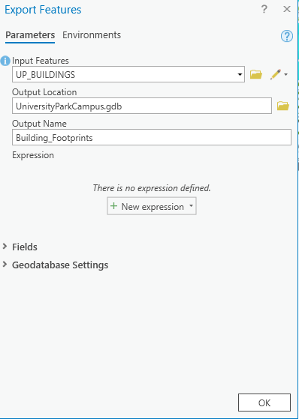 Credit: 2020, ArcGIS [2]
 - On the contents pane, uncheck UP_BUILDINGS Layer. Click Building_Footprints on the Contents pane.
- If the Building_Footprints layer is not extruded,in the Appearance tab, in the Extrusion group, click the Type button and choose Max Height. Click the menu next to Type and choose Z_Mean.
 Credit: 2016, ArcGIS [2]
 - Turn the UP_Roof_ Segments layer back on. Your map should look like this:
 Credit: ChoroPhronesis Lab [1]
 - Save your project.
5.2 Apply a Rule Package to the UP_Roof_Segments Layer
5.2 Apply a Rule Package to the UP_Roof_Segments Layer
In this section, you’ll add special 3D textures and models to your scene to give it a more realistic appearance. The symbology of the structures is presentable in 3D but doesn't give the impression of a realistic city model. For instance, types of roofs, roof textures or façade textures, are not defined in this type of 3D presentation. To make the campus look more realistic, you can set the layer's symbology with a rule package created in CityEngine (see Lesson 2). Rule packages contain a series of design settings that create more complex symbology. Although you cannot create rule packages in ArcGIS Pro, you can apply and modify them from an external file (more in the next lessons).
- Download Building_From_Footprint rule package [6].
- Locate the compressed file in your Downloads folder. Save the file in the project folder you have created earlier in this Module. It is a single file named Building_From_Footprint.rpk.
- If necessary, open the University Park Campus project in ArcGIS Pro.
- In the Contents pane, click the symbol under UP_Roof_Segments to open the Symbology pane.
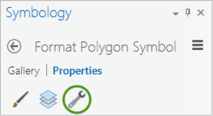
- In the Symbology pane, click Properties and click the Structure button.
Structure presents symbol layers, or graphical components, that create a symbol.
 Credit: 2016, ArcGIS [2]
For the UP_Roof_Segments, the only symbol layer is the light green solid color you have used. To add a rule package to the Symbology, you will create a new symbol layer to which a rule can be applied. - In the drop-down menu in the heading of the symbol layer, choose fill layer
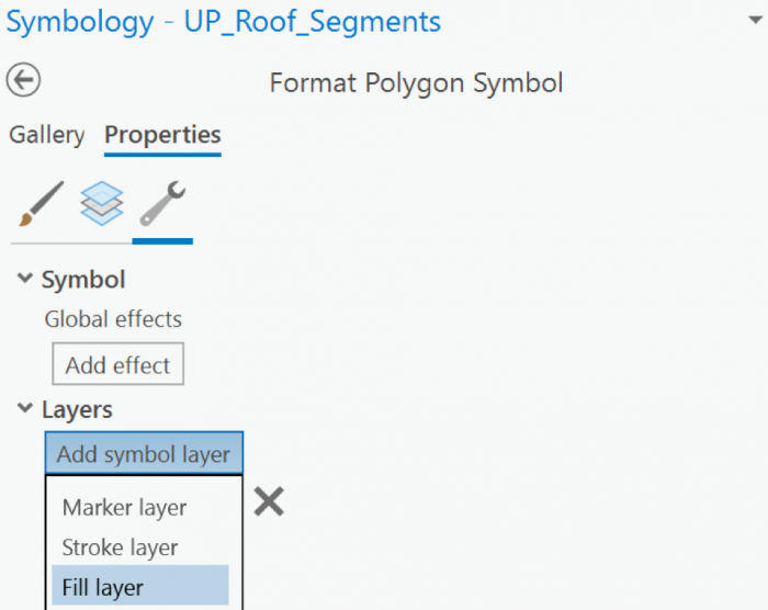 Credit: 2019, ArcGIS [2]
 - Next, you will apply the rules to the Fill symbol layer using the file you downloaded. Under Properties, click the Layers button. Then, select the Procedural fill. Uncheck the line and green color.
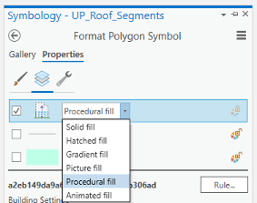 Credit: 2021, ArcGIS [2]
 - The icon from a gray solid color would be changed to an icon indicating a rule assignment. Click the Rule button and Browse to the location of the extracted Building_From_Footprint.rpk file and double-click it. The Symbology pane populates with several symbology settings or rules, that can be adjusted.
- Click apply.
- On the Symbology pane, you need to set rules. Because the rules that are created in CityEngine are based on metric parameters, we have created fields with metric values in the Up_Roof_Segments attribute table.
 Credit: 2016, ArcGIS [2]
 - As you can see, next to each parameter is a ‘set attribute driven properties’ sign. Click to set values from the attribute table.
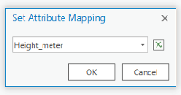 Credit: 2021, ArcGIS [2]
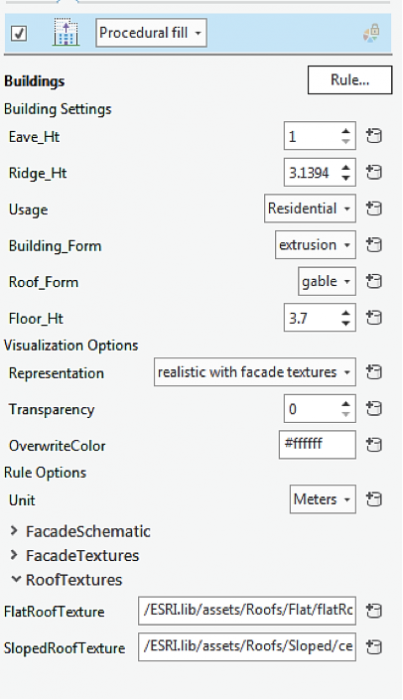
 - Eva_Ht is the distance from the ground to the bottom of the roof. Select Height_Meter from the attribute table.
- Ridge_Ht is the distance from the ground to the top of the roof. Select Ridge_Height_Meter. It is mostly applicable to the slopped roof.
- For Usage select educational. You can see switching from another usage like residential to educational, the thumbnail on the bottom of the pane will change.
- Building_From, select extrusion.
- Change the Floor_Ht to 4.
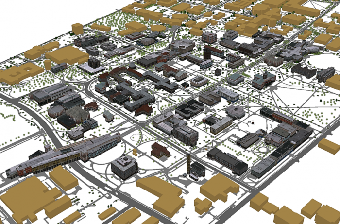
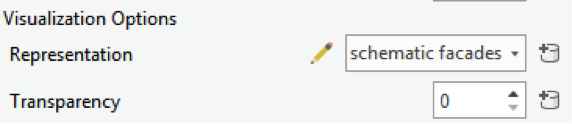
- You will have three options for visualization: (1) realistic with façade textures, (2) schematic facades, (3) solid colors. For now, choose the first option and you will explore the rest later. Click Apply.
 Credit: 2016, ArcGIS [2]
 - Explore the map to get a closer look at the symbology. Roof symbols and Façade symbols. As you see the façade material does not match the actual buildings you can see on Google Earth. That’s because real images of buildings of campus have not been taken. These images are from ESRI library for an international city which is a sample library with different building size and usage textures. The roofs are texturized base on some categories: flat, hip, shed, or pyramid. There is an asset folder of different roof textures and façade textures that are used in setting these rules. For instance, one of the Hip roof colors that you see in the following image. It has been assigned to Hip roofs along with a few more textures.
 Credit: 2016, ArcGIS [2]
 - Save your project.
5.3 Apply a Rule Package to UP_TREES Layer
5.3 Apply a Rule Package to UP_TREES Layer
In this section, you will insert a 3D model of trees with assigned rules. In your 3D Scene, you can see that 2D symbols of trees are presented in 3D. One of the ways to show your trees in 3D is to use LiDAR information such as crown diameter and tree height along with CityEngine procedural rules. However, ArcGIS Pro does not support assigning rule packages to point layers on the Symbology pane, yet. ArcGIS Pro is under constant development and will offer this functionality in the future. A workaround is to export the tree point layer as Polygons with Z information. Then the polygons can be converted to points. The point feature class with Z information and inherited rules can be added to your map as a preset.
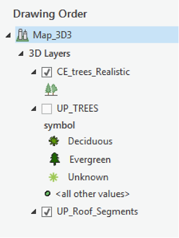
- Uncheck the Up_TREES layer in the 3D Layers list.
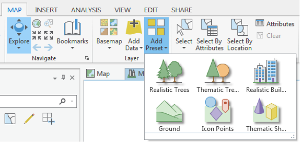
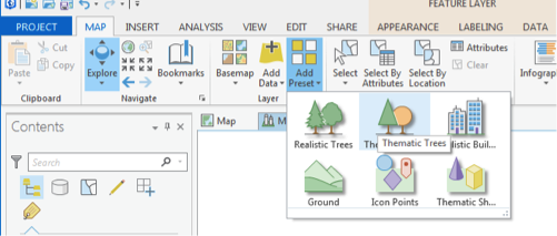
- Under the Map tab, click Add Preset and select Realistic Trees.
 Credit: 2016, ArcGIS [2]
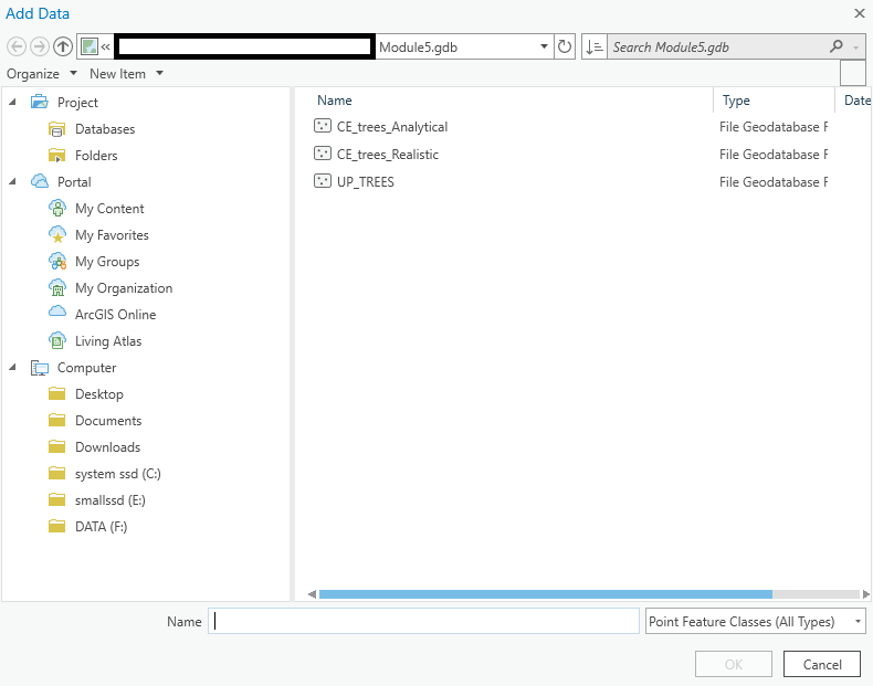
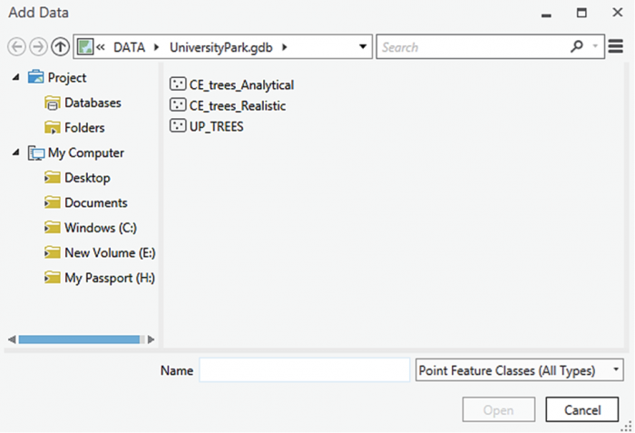
 - From the Geodatabase that you have downloaded, select CE_trees_Realistic. Click Select.
 Credit: 2016, ArcGIS [2]
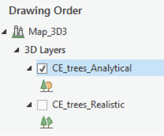
 - The layer will be added to your 3Dlayers list.
 Credit: 2016, ArcGIS [2]
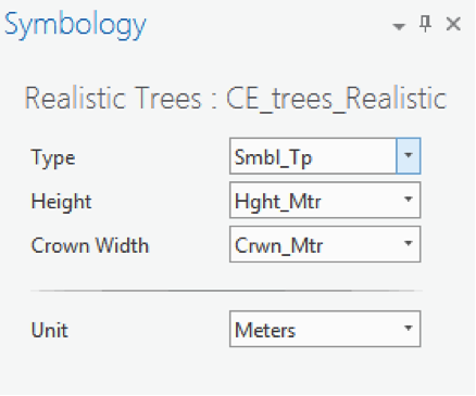
 - As you see on the map, the scale of trees is not right. Click on the symbol under the layer to modify it. Change the parameters as shown below.
 Credit: 2016, ArcGIS [2]
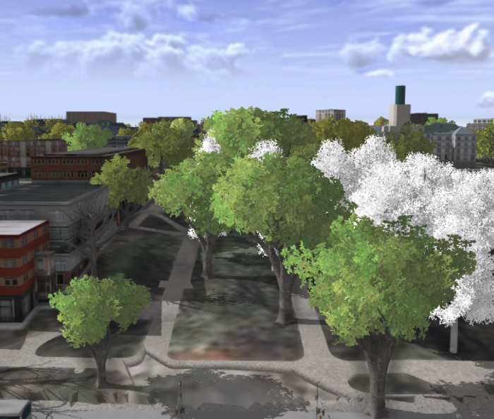
 - As you can see the trees height and crown diameter are now more realistic. You have three tree types under Smbl_TP: Deciduous, Evergreen, and Unknown. The unknown trees should be symbolized white as ghost trees. Unfortunately, both evergreens and unknown trees are colored white, although you can see that evergreen trees have a different shape than deciduous ones. If you change the type from Smbl_TP to Ash, for instance, you can see all trees are changing. You can try different tree types. We will update this section when the feature becomes available in ArcGIS Pro.
 Credit: ChoroPhronesis Lab [1]
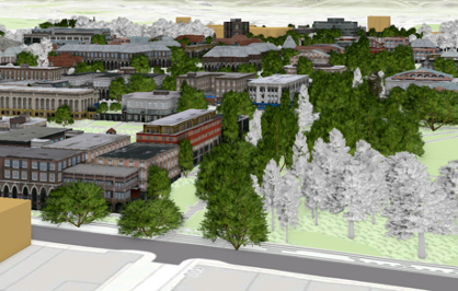 Credit: ChoroPhronesis Lab [1]
 - In the image above, you can see how the trees are symbolized in GIS. In CityEngine (as an example shown below), you can see that not only deciduous and evergreen trees are different but also various tree types under each category are symbolized differently. ESRI is continuously moving functionality from CityEngine to ArcGIS Pro so that it is hopefully only a matter of time that this function becomes available. We are not focusing on CityEngine in this course but will offer you an overview of how it works using the campus data as an example.
You can see the example of tree symbols used in CityEngine to symbolize trees. This vegetation library is imported from LumenRT 3D Plants to CityEngine.
 Credit: ChoroPhronesis Lab [1]
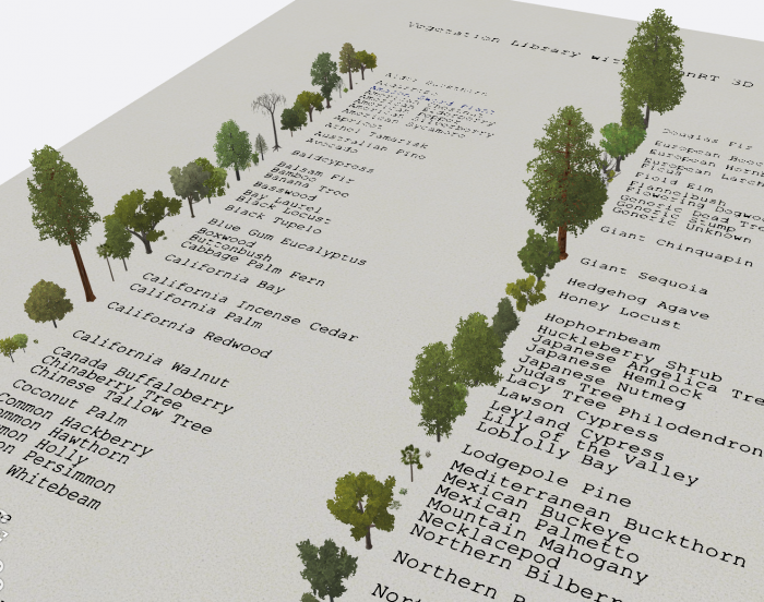 Figure: 3D vegetation with LumenRT ModelsCredit: ESRI/LumenRT vegetation library for CityEngine [12]
 - Create a PDF map (like the end of Section 3) or take a screenshot of your UP Campus realistic 3D model for the final assignment. This is labeled Task 3 on the Tasks and Deliverables of your graded assignment.
- Now you will save your project with a relevant name.
- Click the Project tab. Select Save As.
 Credit: 2016, ArcGIS
 - In the Projects Folder (C:\Users\YOURUSER\Documents\ArcGIS\Projects\UniversityParkCampus), Save Project as UniversityParkCampus_Lesson5. This way you will create a new project for the next lesson.
5.4 Change the Symbology from Realistic to Analytical
5.4 Change the Symbology from Realistic to Analytical
You have learned how to apply a rule package symbology to buildings to demonstrate a realistic view of campus. For some types of 3D analysis, an analytical demonstration may suffice. For the next Module, you will need an analytical presentation of campus. In this section, you will learn how to switch from realistic to analytical. In the next lesson, you will learn examples of 3D spatial analysis and you will need these analytical 3D models for the analysis.
- Click the Project tab. Select Save As.
Credit: 2016, ArcGIS [2]
- In the Projects Folder (C:\Users\YOURUSER\Documents\ArcGIS\Projects\UniversityParkCampus), Save Project as UniversityParkCampus_Lesson6. This way you will create a new project for the next lesson.
- Go back to the Map view.
- Uncheck the CE_trees_Realistic.
- Click on symbology under UP_Roof_Segments. On the Symbology pane, click Properties and select Layers.
- Change representation from realistic with façade textures to schematic facades.
Click apply.
 Credit: 2016, ArcGIS [2]
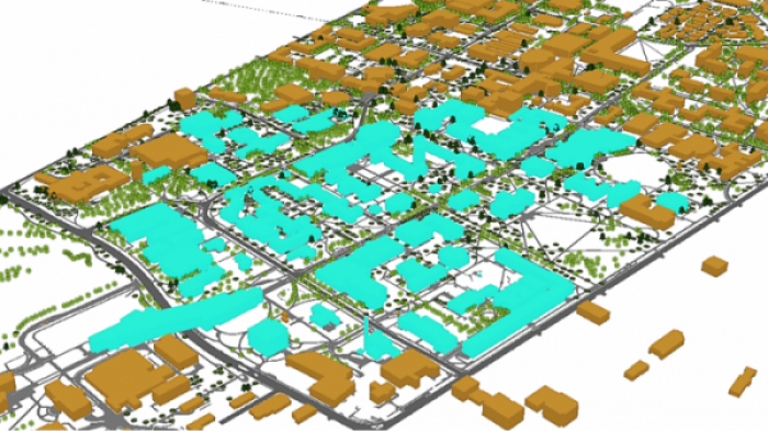
 - Your campus model should look like the following image:
 Credit: ChoroPhronesis [1]
 - Now, you will add thematic trees. On Map tab click Add Preset and select thematic trees.
 Credit: 2016, ArcGIS [2]
 - From the Geodatabase that you have downloaded, select CE_trees_Analytical. Click Select.
 Credit: 2016, ArcGIS [2]
 - The layer will be added to your 3Dlayers list.
 Credit: 2016, ArcGIS [2]
 - As you see in the map, the scale of trees is not right. Click on the symbol under the layer to modify it. Change the parameters as shown below.
As you see, one of the factors is color by value. Select random Seed and the green color ramp. This will give your trees a more colorful presentation.
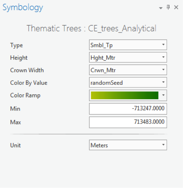 Credit: 2016, ArcGIS [2]
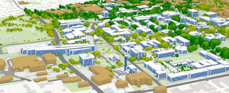 Credit: ChoroPhronesis [1]
 - Create a PDF map (like the end of Section 3) or take a screenshot of your UP Campus schematic 3D model for your graded assignment. This is Task 4 on the Tasks and Deliverables page.
- Save the project.
In this lesson, you learned how to work with ArcGIS Pro from creating a map and symbolizing layers to exploring raster and 3D data. You also learned about symbolizing 3D layers with rule packages from CityEngine. In the next lesson, you will learn about some 3D analysis that is possible with 3D data.
Tasks and Deliverables
Tasks and Deliverables
Assignment: ArcGIS Pro adn 3D modeling
This assignment has 3 parts, but if you followed the directions as you were working through this lesson, you should already have most of the last part done.
Part 1: Submit Your Deliverables
If you haven't already submitted your deliverable for this part, please do it now. You need to turn in all four of them to receive full credit. You can paste your screenshots into one file or zip all of the PDFs and upload that. Task 2 will need to be a PDF, so either way, you will have two files to zip.
- Task 1: a screenshot of all layers symbolized for UP Campus (end of Section 2)
- Task 2: print a PDF map of Smoothed_DEM Layer with a legend showing the minimum and maximum elevation (end of Section 3).
- Task 3: print a PDF map of your 3D campus with realistic facades and trees or simply create a screenshot (end of Section 5.3)
- Task 4: print a PDF map of your 3D campus with schematic facades and analytical trees or simply create a screenshot (end of Section 5.4)
Grading Rubric
Grading Rubric Criteria Full Credit No Credit Possible Points Task 1: Screenshot of all layers symbolized for UP Campus correct and present 1 pt 0 pts 1 pt Task 2: PDF map of Smoothed_DEM Layer with a legend showing the minimum and maximum elevation correct and present 1 pt 0 pts 1 pt Task 3: PDF map of your 3D campus with realistic facades and trees or simply create a screenshot correct and present 1 pt 0 pts 1 pt Task 4: PDF map of your 3D campus with schematic facades and analytical trees or simply create a screenshot correct and present 1 pt 0 pts 1 pt Total Points: 4
Part 2: Participate in a Discussion
Please reflect on your 3D modeling experience, using ArcGIS Pro; anything you learned or any problems that you faced while doing your assignment as well as anything that you explored on your own and added to your 3D modeling experience.
Instructions
Please use Lesson 5 Discussion (Reflection) to post your response to reflect on the options provided above and reply to at least two of your peer's contributions.
Please remember that active participation is part of your grade for the course.
Due Dates
Your post is due Saturday to give your peers time to comment. All comments are due by Tuesday at 11:59 p.m.
Part 3: Write a Reflection Paper
Instructions:
Once you have posted your response to the discussion and read through your peers' comments, write a one-page reflection paper on your experience in 3D modeling with the following deliverables as a proof that you have completed and understood the process of 3D modeling for Campus.
Due Dates
Your assignment is due on Tuesday at 11:59 p.m.
Submitting Your Deliverables
Please submit your completed paper and deliverables to the Lesson 5 Graded Assignments.
Grading Rubric
| Criteria | Full Credit | Half Credit | No Credit | Possible Points |
|---|---|---|---|---|
| Paper clearly communicates the student's experience developing the 3D model in ArcGIS Pro | 5 pts | 2.5 pts | 0 pts | 5 pts |
| The paper is well thought out, organized, contains evidence that student read and reflected on their peer's comments | 5 pts | 2.5 pts | 0 pts | 5 pts |
| The document is grammatically correct, typo-free, and cited where necessary | 1 pts | .5 pts | 0 pts | 1 pt |
| Total Points: 11 |
Summary and Tasks Reminder
Summary and Tasks Reminder
In this lesson, you have learned how to symbolize 2D and 3D maps. You also have learned the differences between static modeling and procedural modeling. Most importantly, you practiced how to create a 3D model of elevation and how to incorporate City Engine procedural rule symbology into GIS.
Reminder - Complete all of the Lesson 5 tasks!
You have reached the end of Lesson 5! Double-check the to-do list on the Lesson 5 Overview page to make sure you have completed all of the activities listed there before you begin Lesson 6.