Question
Assume the chemical weathering occurred for 0.1 million years. Please set up the simulation in Crunchflow. Plot the profiles of pH, Saturation index (SI, equal to [log10(IAP/Keq)]), $\phi$ ( volume of mineral/ volume of total porous media) of minerals and $\tau$ of K and Si relative to Zr in this soil column at the initial time, 5 thousand years, 10 thousand years, 20 thousand years, 40 thousand years and 100 thousand years. In calculating $\tau$ of K and Si relative to Zr, please assume the soil column always has a constant concentration of immobile reference element Zr, which means $\mathrm{C}_{\mathrm{Zr}, \mathrm{p}} / \mathrm{c}_{\mathrm{Zr}, \mathrm{w}}=1$ all the time. Discuss what you observe.
Note:
Setting up this lesson will involve what you learned from the lesson on mineral dissolution and precipitation, as well as the lesson on 1D transport. If needed please revisit these two lessons. In this lesson we do not provide videos and template anymore.
Please watch the following video: Mineral Dissolution and Precipitation 1D Columns (20:09)
Click here for CrunchFlow files
Click for a transcript of the mineral dissolution and precipitation 1D Columns video
Mineral Dissolution and Precipitation 1D Columns
Li Li: OK, so this lesson we're going to talk about mineral dissolution, precipitation in one dimension, like, 1D columns. So this is different from the previous lessons that we had before on mineral dissolution and precipitation, which was in batch reactor, well-mixed systems. So it is really no dimension. Or you can call it a zero dimension because, in every spatial point, they are the same. So here, we are talking about 1D. What that means is that, essentially, you have a column. So we're talking about processes like, for example, rainfall comes in, hitting parent rock, and things dissolving out. And then, over a long period of time, these chemical species release out. And rock becomes soil.
So I'm going to use this as one example to talk about mineral dissolution and precipitation in 1D columns and how we set up these equations. But it's not really only about chemical weathering. It's really about these mineral dissolution precipitation reactions in general. In the short-terms, these reactions actually change, for example, water chemistry. If you think about a ground-water system, it would actually tend to-- we can see the change if there is mineral dissolution precipitation -- happen pretty fast. But in order to see change in the solid phase, we do need to wait a bit longer for enough change to happen. So today, I'm going to use this system. So I'll talk about this. If we're talking about rock transformation to become soil, we are setting up a system that has rainfall come in at a rate, maybe, for example, some way that is about annual precipitation minus e-t, something like that, at this flow velocity. And first thing, usually, we would have an unsaturated system in these topsoils, but for simplicity, we would just think about everything at the fully saturated system.
So it's easy at the beginning. So we have these systems that have essentially two minerals as parent rock. One is quartz -- and dissolves pretty slowly. Everyone knows about that. The other is K-feldspar, which is a very common silicate in rocks. K-feldspar has a formula of KAlSi and then O3-8. So essentially, you can think about this system-- if you think about rainfall, it comes in, dissolving out, and then releases these chemical species, that you can think about several processes as happening at the same time. One is advection. So this is the same advection we talked about in one unit set with a chaser, essentially, as the flow brings out the chemicals, but also there's a dispersion, diffusion. This again, is the same as what we talked about last time in the AD equations. But then the last one that is different from the previous, one other reaction, which is mineral dissolution precipitation reaction. So essentially this is like combining the AD equation unit with the mineral dissolution precipitation reaction unit. So if you need to go back, you're welcome to review this material. But essentially, because these three different processes are happening at the same time-- but then we also have multiple minerals -- we know the qualities are pretty slowly. And we can more or less think about this as almost non-reactive. Because compared to K-feldspar, it's a relatively very slow reaction. And when we think about the reaction that's happening, the K-feldspar will be dissolving out. So you would have this K-feldspar dissolving out to become released calcium, which is very important nutrients, metals, cations. And then it would be also released aluminum plus SiO2, so that's aqueous. These are species that are going to be coming out.
But at the same time, you also think about, some of these chemical species, when they reach a certain level, actually they can precipitate out as solid phase again. For example, aluminum plus SOi2 actually will become another mirror, which we call kaolinite. So essentially it will have the formula of Ai-Al2-Si2-O5-OH4. This is kaolinite. This is one type of very common clay in our system. Or if you go digging some soil, you will very easily see this type of clay. So essentially, you can think about the whole process as, like, you have parent bedrock. Rainfall comes in, releases some of the chemical species. But then some of these species also re-precipitate out. So it's almost like a redistribution of minerals. But at the same time, because some of species dissolving out over a long period of time, it would change the properties of the system, for example, porosity, permeability. Make this solid phase more permeable and have more pore space for water to flow through. So there's a change in physical properties as well.
So one question we often ask is how does this water and rock change over time and also over space? We want to know how fast things change and how much they change and what they have become. And a lot of time, we want to be able to predict that. So in order to do that, we have to come set up the equations, reactions, and all of that, putting everything together, and think about how we solve them.
So again, with the system, every time we need to think about the chemical system and how they evolve over time and space, we think-- the first thing we need to think about-- the chemical species first. So you have several primary species again. If you review back some of the material we covered before, we had primary species, then existent system-- because we have aluminum, silica-- that they have to be there. This has to be part of the building block of the system. You have potassium too. And when the rainfall comes in, usually it brings some acidity. So H-plus should be there. You would also have CO2-aq. In addition, a lot of times, these rainfalls have a little bit of salt in them. So to be representative, we are also putting a bit of sodium chloride in that example-- sodium chloride as part of the rainfall. That means, also, in the second species, we need to decide, OK, what complexities would be formed, how much can complex reaction happen, and things like this. So to keep it simple, I'm going to just have potassium and then HCO3-aq and maybe KCl-aq as two complexities. And then, of course, we also need other species, for example, H-minus. We need the other form of bicarbonate and carbonate. So it's quickly become a long list of species.
So if we are talking these chemical species, we'll be essentially solving for 1, 2, 3, 4, 5, 6, 7. We'll have seven primary species. So that essentially means we would have seven independent equations to solve for. So what I'm writing here is a general type of governing equation, for one species, I. And again, this first term-- we call, mass accumulation term, that we discussed before. Is a summation of overall change. And then you have the advection term, diffusion term, dispersion term. These doesn't change, because of the system. But for example, the primary would change, but the terms wouldn't change. You could have different porosity phi or velocity or diffusion-dispersion coefficient for a different chemical species. But the term itself wouldn't change. And then the last term is new. It's a reaction term. So it would take into account, essentially, different types or the rates of different types of reactions that this species, I, is involved in. And you think about how fast these different reactions would change in the continuation of species I. And of course, this I needs to be written for 1 to Np, which is the number of primary species. So you need to write, for this system, seven different equations to solve. But then, on top of that, again, you have this number of secondary species you need to solve for in the form of algebraic relationships.
So how does this r-i-j look? These are terms different from the previous AD equations, that without this term. Now here, this r is a [INAUDIBLE] term. So you have that. So for this, r's, it needs to be-- everything about this particular r-- let's make this i is potassium. So for potassium, means this system-- you can think about two reactions involved in. One is that the K-feldspar dissolving out to release out calcium. And then it comes out. And it goes. So actually, one reaction-- so it would be just K-feldspar dissolving out. So if it's K, then you would just have this rate. And then you follow TST rate all right. So you have, probably, this complicated K-H-plus, dependence on H-plus, whatever term, empirical numbers, K-H2O and then a water plus KOH-minus and then Activity OH-minus-- some empirical exponent here as well. These are the regular part, early part, that depends on pH. But then, again, you have surface area. And the last term would be 1 minus IAP over K-aq. Again, it's how fast this is close to equilibrium or far away from equilibrium. So that's the general form of reaction rate law. So when we solve equals to this term, we'll be putting there-- so this is going to be a complicated term. But also, if you think about, for example, species like aluminum or silica, then they're actually involving two different reactions. One is K-feldspar dissolving out to release these. But a kaolinite also precipitated out. So there's one source reaction term and r-i term. And the other would be a sink term for kaolinite precipitating out. So it's a sink for aluminum or silica.
So we solve all of these equations. And what we come up with is all these Ci as a function of time and space. So you have X versus-- essentially, once we know all the parameters, initial conditions, bounded conditions-- what water comes in, what water comes out the beginning, what's the pore water composition in the rock and all that, this will give us this distribution of concentration from time and space. And over geological time, when this changes line-- and when I say geological time, I mean at least thousands of years, thousands or 10 thousands or close to 1 million years, things like that. So over this time scale, you would have these things keep on changing. And then the rock becomes soil, property of the porous media change. You have porosity increases typically. And you have, also, permeability change, because the water-- the resistance of this porous media to water becomes lower and lower. So you have permeability increase as well. So this would be the chemical weathering over long-term. Over short-term, is all of these reaction changes or water chemistry.
But the last part of it, I want to mention a little bit about the dimensionless number, from the mass point-of-view, how these would change, how we analyze these systems. So last time, when we talked about this equation of AD with other reaction term, we talked about the Pe or Peclet number, which is the tau of the advection. It's a tau diffusion-dispersion over tau advection. Tau is a time scale, right? So the time scale of diffusion and dispersion, which is L squared over D-- so it's length of this column-- over diffusion-- because that's the time scale for diffusion-dispersion-- divided by-- or times, if I do it this way-- times 1 over tau-a, which is the opposite of lance over advection. So you would have v-L. So that cancels out. It becomes L-v over D. And so that's a Peclet number, that we talked of before. So this term essentially compares the relative magnitude of advection versus diffusion-dispersion. Which point is dominant under phosphoro or slow conditions? But then, because we have the reaction term, we have two more different dimensionless numbers, we call Damkohler numbers. So the first step-- because think about, we have two transport processes. One is diffusion-dispersion. Other is the advection. So the first one is comparing the time scale of reaction-- the relative time scale of advection to the relative time scale of reaction. And in that case, again, tau-a would be the same as L over v. But then, you'd be-- this is over tau reaction. For reaction, we are thinking about how much things can dissolve and, eventually, reach equilibrium. So you would have total bulk volume times porosity, which is how much pore space you have that can hold water. So that's a lot of volume times the maximum concentrations and you can dissolving out, divided by the rate constant as a maximum, K times A. So this would be, essentially, the reaction time, the characteristic time for reaction. And in notes, I have simplified this. And you can have that. You can look at these. For the second Damkohler number, you would be comparing the time scale of diffusion-dispersion over tau-r. And again, this would be going back to L squared over D, divided by the same thing. Because the reserve reaction term would be the same.
So if you think about-- we typically talk about, under fast reaction system, fast compared to transfer versus when you have very slow reaction systems. So when you have very fast reaction systems, the systems tend to reach equilibrium quickly. And we tend to be transporter-controlled. It would be determined by the bottleneck of all processes, which mean it's going to be transport-controlled. If the reaction is actually slower-- so you will see, by this analysis, you will be able to tell how the system would behave, whether it's transport-controlled or surface reaction-controlled. And how these will be changing over distance and time will give us some kind of grouping analysis that we can do.
So I'm going to end here. I'm going to go back and look at notes. And this, I went through pretty fast. So look at notes we have. Do some homework. And you will realize, these analyses will really help you to understand how things are different under different conditions.
Click for Solution
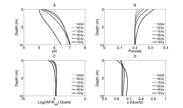
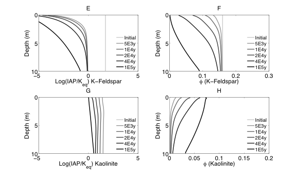
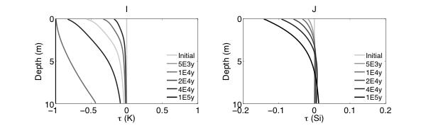
Figure 2 Evolutions of (A) pH (B) porosity (C) Saturation Index $\left[\log 10\left(I A P / K_{e q}\right)\right]$ of K-Quartz, (D) $\phi$(Quartz) (volume of Quartz / volume of total porous media) (E) Saturation Index $\left[\log 10\left(I A P / K_{e q}\right)\right]$ of K-Feldspar (F) $\phi$ (K-Feldspar) (volume of K-Feldspar / volume of total porous media) (G) Saturation Index $\left[\log 10\left(I A P / K_{e q}\right)\right]$ of Kaolinite, (H) $\phi$(Kaolinite) (volume of Kaolinite / volume of total porous media), $\text { (I) } \tau(K)$ and $\text { (J) } \tau(S i)$ as a function of soil depth at different times.
Initially, the pH in the rock is 6 and porosity is 0.2. After the simulation starts, rainwater flows into the soil column from the top with a lower pH so the pH in the upper column (close to the surface) decreased. In the lower part of the column, incoming hydrogen ion is consumed during mineral dissolution so pH increases. As mineral dissolves, porosity is enlarged. Porosity increases more where mineral dissolution is faster. Because rainwater has lower pH and lower solute concentrations, Quartz is under saturated and dissolves from the top. However, because the lower part of column has a higher pH, Quartz is re-precipitating in the lower part of column. K-Feldspar is under saturated throughout the column so it always dissolves. Kaolinite precipitates as a secondary mineral as K-Feldspar and quartz dissolve and elevate the aqueous concentrations.
From the discussion above it is apparent that soil at different depth weathers differently primarily due to the availability of reactants for the dissolution reactions at different depth. The delivery through flow and transport and the consumption of reactants compete with each other in the soil profile, which determines the location and shape of the weathering front. In fact, the extent and speed of chemical weathering can often be interpreted inversely based on understandings of the vertical profile through numerical simulations [Brantley and White, 2009].