Power Curve
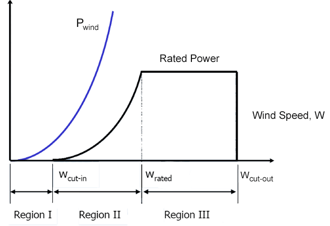
Figure 2a-1 below illustrates a typical power curve of a modern, pitch-controlled, horizontal-axis wind turbine. It is plotted as power versus wind speed. The solid blue line (Pwind) denotes the power available in the wind. Wind power is proportional to the cube of the wind speed, as shown by the Pwind line. What does this mean? If you double the wind speed, the result is an eight fold increase in the power you can capture from the wind.
The following video explains the 3 wind (or power) regions from Fig. 2a-1:
Transcript: Power Curve of Pitch-Controlled HAWTs
A real wind turbine, if you look at it, it's going to take a bit of a wind speed to start it. So there is a region from zero wind up to a certain wind speed, called the cut-in wind speed, where there is no power produced by the wind turbine. Also called the region 1. Nothing is happening. Then, once the cut-in wind speed is reached, power ramps up and you see that it's in an almost parallel slope to the power that becomes available with the wind speed itself. But it's only a certain fraction of that amount that actually a machine, a wind turbine rotor, can capture. We're going to learn about how much that is. That region is called region 2. Power ramps up.
Ideally, you want to produce power with wind turbine and you want to make money. Right, you want to sell the power. Ideally you want to go all the way up here, but you're limited. What limits you? Generator. The first thing that limits you is the generator. Generator can only take so much power, and feed it into the electrical grid. You have to start controlling the power. That's the typical power curve of a modern pitch controlled horizontal axis wind turbine. You control the power by changing the blade pitch. Changing the load and hence the torque and power produced by the rotor. That wind speed where you reach the rated power of a turbine and the generator is called the rated wind speed. From there on as the wind speed increases, we're going to see you have to pitch more and more the blades to accommodate for the fact that more wind power is coming in, but you can only allow to capture so much of that. Essentially you have to adjust the blade pitch angle such that local angles of attack acting on local airfoil sections become smaller, and hence the loads the become relatively smaller and the power stays the same.
So then back at the end here, usually if the wind speed becomes about 25 meters you have to shut down the turbine. Why is that? It's not a generator problem. It's the blade loads. Becomes a load and fatigue issue. Storm condition also. In a storm, you have more fluctuations, large amplitude and that poses a problem, you have to shut down the rotor. That's the cut-out wind speed. So we have these 3 distinct regions, in a power curve of a modern pitch controlled horizontal axis wind turbine.
Actuator Disk Model
The flow field around a wind turbine rotor is very complex. The blades of today’s utility-scale wind turbines are equipped with various airfoils that are optimized to perform at their respective position along the blade span. Depending on the wind speed, blades are pitched collectively to either maximize the power extraction at a given wind speed or to control the power production for wind speeds larger than rated. Furthermore, the blades experience elastic deformations and are exposed to wind gusts, turbulent eddies, and an incoming sheared wind profile of the surrounding Atmospheric Boundary Layer (ABL).
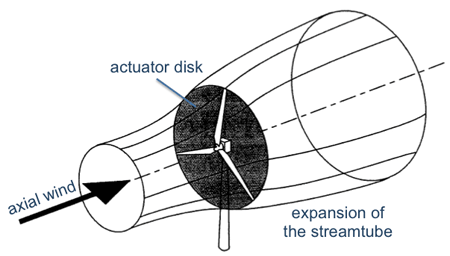
The apparent problem complexity includes time-varying, three-dimensional, turbulent flow with vortical structures. It seems impractical to gain some basic understanding in power production and blade loads without significantly simplifying the problem. For this purpose, let us think about the wind turbine as a device that extracts momentum and energy from the wind, and does so ‘uniformly’ over the rotor swept area (as indicated in Fig. 2a-2). We can hence consider the rotor as an infinitesimally thick actuator disk (surface) that reduces the momentum of the axial wind.
A one-dimensional and axi-symmetric model in fluid dynamics is that of the streamtube, see again Fig. 2a-2. As the wind turbine extracts momentum and energy from the axial free stream, the wind inside the streamtube slows down. Consequently, the streamtube has to expand in order to satisfy mass conservation in the former.
We add a further assumption to the problem that concerns neglecting shear effects within the streamtube. This means, in particular, that there is a uniform wind profile entering and exiting the streamtube. Hence, viscous losses are neglected (inviscid) that prohibit the generation of vorticity and associated vortical structures such as root- and tip vortices (irrotational). We further assume that the actuator disk be stationary (no rotation) and that the uniform wind entering the streamtube does not change in time (steady).
Let us summarize the assumptions the Actuator Disk Model: steady, 1-D, inviscid, irrotational, no rotation.
Basic Streamtube Analysis
Let us refer to Fig. 2a-3 (top plot) for a cross-sectional view through the streamtube. We can see that a uniform wind profile V0 enters the streamtube. The wind speed inside the streamtube continuously decreases (lower plot) as the wind turbine extracts momentum and energy from the wind profile that enters the streamtube. At the actuator disk, the uniform wind profile is of magnitude u; at the exit plane of the streamtube, the velocity magnitude has reduced to u1. We note that the wind speed V0 outside the streamtube remains unchanged.
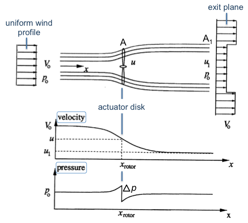
Before proceeding, let us have a closer look at the exit plane where two uniform velocity profiles come together. An abrupt velocity gradient is present, however our assumption of inviscid and hence irrotational flow allows for ‘free’ slip along the streamtube. Therefore, no friction losses are present in the analysis. – While the velocity distribution along the streamtube is continuous, the situation is different for the static pressure. It is obvious that the local static pressure has to equal the ambient pressure p0 at the streamtube entrance and exit. However, the continuous flow deceleration inside the streamtube demands an increase in pressure according to Bernoulli’s law (which we will refer to a little later). Therefore, the only way to satisfy that the static pressure at streamtube entrance and exit equals p0 (ambient pressure) is to have a pressure discontinuity Δp at the actuator disk. It is this pressure jump that acts as an external force to the fluid and extracts the axial momentum, respectively energy and power.
In the following, let us write down some familiar engineering relations.
We can write the Rotor Disk Area as a function of rotor diameter D as:
As for the Mass Flow Rate (m*) through the streamtube, we can evaluate it at the actuator disk:
and at the exit plane (noting that the exit area A1 at the streamtube is thus far unknown to us):
The pressure jump Δp across the actuator disk acts on the rotor disk area A to produce the thrust force T of the wind turbine:
We note that the thrust force acts downwind in the streamwise direction. This is a consequence of the fact that a wind turbine extracts axial momentum and energy, which is opposite to the behavior of a propeller that generates an upwind thrust force by accelerating the fluid at the expense of engine power. From Newton’s second law, we know that a force equals a change in momentum. Considering the streamtube as a control volume we find that the thrust force T is the only external force acting on the control volume and that this force is balanced by the momentum fluxes that enter and leave the control volume:
As for the power P (which is what we really want in Wind Energy), we remember that power equals energy per unit time. The wind turbine extracts ‘kinetic’ energy from the wind, hence the amount of power being extracted equals the difference in kinetic energy fluxes entering and exiting the streamtube control volume:
In order to compute rotor thrust T and power P we need to find the velocities u and u1 at the actuator disk and at the exit plane. In addition to mass conservation and Newton’s 2nd law we can apply the classical incompressible Bernoulli equation to the flow inside the streamtube. We note, however, from Figure 2.2 that the pressure is discontinuous across the actuator disk. Hence the Bernoulli equation can only be applied upstream and downstream of the pressure discontinuity.
Video Question: What are the conditions in order to apply Bernouli's Equation?
Transcript: Conditions for using Bernoulli's Equation
When can you use Bernoulli's Equation? Steady, Inviscid, irrotational, incompressible, and there's a fifth one. Anybody remember the fifth condition? That's the one that is not going to make it work here. Conservative body forces. What is an example of a conservative body force? Gravity is a conservative body force. How about pressure jump? Is that conservative? No, it's not. It's like a shock wave. That means you can NOT apply Bernoulli's Equation all across here, but break-up the problem and apply Bernoulli's Equation upstream of the actuator disk and downstream of the actuator disk. That's exactly what we are going to do next.
Bernoulli Equation
We begin by writing the Bernoulli equation ‘upstream’ of the actuator disk as:
In this equation, p is the pressure slightly upstream of the rotor disk. If we define the pressure drop across the actuator disk as Δp, then the pressure just downstream of the actuator disk becomes p-Δp. We can then write the ‘downstream’ Bernoulli equation as:
Subtracting the upstream and downstream Bernoulli equations from one another relates the pressure drop Δp to the unknown velocities u and u1:
We can use the relation for the pressure drop Δp in the equation for the thrust:
...to obtain u:
It is interesting to observe that the velocity u at the actuator disk is the arithmetic average of the velocities entering and exiting the streamtube.
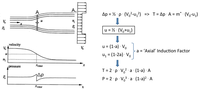
It is practical in many engineering problems to use dimensionless coefficients (figure 2a-4). Let us define an ‘axial induction factor a through u=(1-a)⋅V0 which describes the velocity u at the actuator disk as a fraction of the free stream wind speed V0.
Using u=½⋅(V0+u1) we can write the velocity u1 at the exit plane as u1=(1-2a)⋅V0. It becomes evident that in the special case of a=0, the unknown velocities u and u1 simply equal the free stream wind speed V0 and both thrust T and power P are zero.
A couple things about thrust and power:
Transcript: Thrust and Power
We note a couple of very important things. Number one is thrust is proportional to the square of the wind speed. And that is also reflected in a quadratic dependence on the axial induction factor a. While the the power P is proportional the cube of the wind speed. We had mentioned it earlier. And that is also reflected in a third order dependence on the axial induction factor a.