Rotor Thrust and Power
Next, we use the derived equations for u and u1 in those for the thrust T and power P and obtain:
We hence obtained thrust T and power P as a function of air density ρ, wind speed V0, actuator disk area A, and the ‘axial induction factor’ a. It is convenient to write both physical quantities in an appropriate dimensionless form.
As for the thrust T, we use the dynamic pressure acting on the actuator disk as the normalization factor:
For the power P, we use the available ‘power in the wind’ Pavail passing through the rotor disk area A as the normalization factor:
We can thus define a thrust coefficient CT and power coefficient CP as:
Both are dimensionless quantities and are sole functions of the axial induction factor a.
This means in particular that thrust T and power P can be written as:
The previous equation illustrates the key dependencies for thrust and power:
- The thrust T is proportional to the wind speed squared, the rotor diameter squared, and the thrust coefficient.
In general, one aims at minimizing the rotor thrust for a given wind speed and rotor diameter, i.e. as small values of CT as possible are desired.
- The power P is proportional to the wind speed cubed, the rotor diameter squared, and the power coefficient.
It is obvious that one would aim at maximizing the power coefficient CP given a wind speed and rotor diameter. However, we note that there is just a linear proportionality of rotor power to the power coefficient. The biggest effect on the total power P is due to the wind resource V03 and rotor size D2.
Let us consider again the relations for the thrust coefficient CT and power coefficient CP as sole functions of the axial induction factor a.
We note that CT is a quadratic function in a, while CP is a cubic function in a. Next, we plot the dimensionless quantities CT and CP versus their dependent a in order to find some basic limitations on rotor thrust and power.
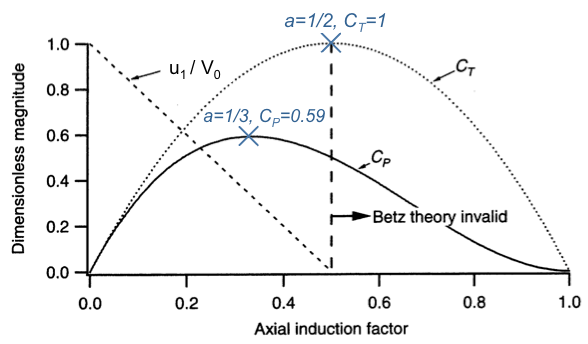
As for the thrust coefficient CT, we find it to be of parabolic shape symmetric about a=0.5. Its maximum value is CT=1, which makes the rotor thrust being equal to the dynamic pressure force on a solid actuator disk. (Figure 2a-5.) See definition of CT in equation (2.16).
Transcript: Thrust Coefficient and Power Coefficient
Let's plot some of the results that we have learned. We want to plot the dimensionless magnitudes of the the thrust coefficient CT and the power coefficient CP verses the axial induction factor a. But first let us remember what these relations were. The thrust coefficient C sub T, we had 4a(1-a). And for the power coefficient C sub P, we found it to be 4a(1-a) squared. In other words, thrust coefficient exhibits quadratic dependence on the axial induction factor a, while the power coefficient shows a cubic dependence.
Let's start first with the thrust coefficient CT. The quadratic demands that it is a parabola. So if a is zero, naturally that becomes zero. Also the thrust coefficient is zero for a being equal to 1. The dotted line here represents the parabola. You can show easily that this parabola will have a maximum for an axial induction factor a=1/2, in which case the maximum thrust coefficient becomes one.
Things are a little different for the power coefficient CP because we have this cubic dependence. But again, if a is zero, the power coefficient is zero and also for a=1, the power coefficient will be become zero. There a are few subtleties to the power coefficient, that is the cubic dependence give us the maximum, the minimum and the inflection point somewhere in between. We will derive, later, that the maximum power coefficient of CP=0.59 is obtained for an axial induction factor a=1/3.
Now just remember that power is something that's good for us, we want to capture as much power as we can. Thrust, well, if we can reduce it to a minimum better, because the thrust force of the rotor is creating a large bending moment to the tower and foundation of a wind turbine.
One more thing I'd like to point out here is that we need to be aware of the exit velocity u sub 1 out of the streamtube. Why is that? We found earlier that u1/V knot is a fuction of A2 and that equals 1-2a. Now, if a, the axial induction factor, becomes larger than 1/2, something happens and that is u1/V knot, the wind speed, becomes less than zero. In other words, the exit velocity out of the stream tube is reversed. If the flow reverses, also called the turbulent wake state, that is something that is absolutely not compliant with the assumptions that we put into momentum theory. And this is why here is the diagram, it's indicated for a>1/2 the Betz theory or momentum theory becomes invalid. The maximum power coefficient, we shall see later, is also called the Betz limit.
So far so good, let's move on to the next subject.
Find CT,Max:
As for the power coefficient CP, we find that its maximum value is approximately 0.59 for an axial induction factor of a=1/3. (Figure 2a-5.)
Find CP,Max:
With reference to the definition of the power coefficient CP in equation (2a.17), it becomes clear that we can at the most harvest approximately 59% of all the kinetic energy in the wind that passes through the streamtube.
The upper limit for the power coefficient CP,max=0.59 is called the “Betz Limit”.
Figure 2a-5 also illustrates a diagonal dashed line representing the ratio of the streamtube exit velocity u1 and the wind speed V0. From Figure 2a-4, we can see that u1/V0 depends linearly on the axial induction factor a. It is not surprising that u1/V0=1 for a=0, as in this case of zero induction both rotor thrust and power equal zero. However, the ratio u1/V0 becomes negative for a>0.5. This means in particular that there is reverse flow at the exit of the streamtube. This flow state is called the “turbulent wake state” and violates the assumptions of inviscid and irrotational flow of the actuator disk model. We thus conclude that the actuator disk model is valid for axial induction factors a<0.5.
Wake Expansion and Wake Shear
Figure 2a-6 shows that as the thrust coefficient CT increases, i.e. increasing axial induction factor a, the streamtube expands with decreasing entrance area A0 and increasing exit area A1. Note that there is always the wind speed V0 entering the streamtube, while we saw that the exit velocity u1 is a linear function of the axial induction factor a. As a consequence, there is a discontinuity between the exit velocity u1 and the ambient wind speed V0.
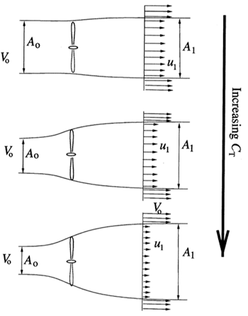
Now remember that the streamtube is a fictitious surface that allowed us to apply mass, momentum, and energy balances within the assumptions of the actuator disk model. In reality, the discontinuity between the streamwise velocities inside and outside the streamtube generates a ‘viscous shear layer’ in the wake. It has been found that wake shear becomes very strong for u1/V0<0.2 or a>0.4. This further limits the validity of the actuator disk model to axial induction factors a<0.4.
Wake Expansion
- Velocity Jump u1/V0
- Rotor Thrust CT
Wake Shear
- Dominant for u1/V0 < 0.2
- Turbulent eddies
Validity of Momentum Theory
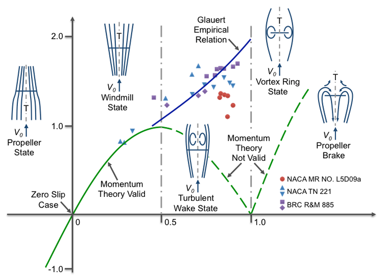
Figure 2a-7 below presents another illustration concerning the validity of the actuator disk (or momentum) theory. Plotted is again the thrust coefficient CT versus the axial induction factor a. For a<0, we are in the propeller state where the streamtube is contracting, and the thrust force is directed upstream and acts as a propulsion device. Note that one has to provide energy to the fluid for a<0. For 0<a<0.4, we are in the windmill state where momentum theory is indeed valid. The streamtube is expanding, and the thrust force is directed downstream and acts as a drag force. In this case, we are extracting energy from the main flow stream.
The second half of the CT parabola (a>0.5) is plotted as a dashed line with an indicator that momentum theory is invalid. This is the ‘turbulent wake state’ that begins with a=0.5 and reverse flow at the exit plane that progresses towards the actuator disk with increasing axial induction factor a. For a=1.0, the reverse flow has reached the actuator disk, and the rotor enters the ‘vortex ring state’. This special flow state can be very dangerous for helicopter rotors. At approximately a=0.4, a solid line ‘Glauert Empirical Relation’ connects the CT curve for momentum theory to the limiting value of CT=2.0 that represents the drag coefficient of a flat plate at 90 degrees angle-of-attack.
The symbols denote experimental data obtained by Glauert in the 1930s. The steep increase of the thrust coefficient CT for a>0.4 is attributed to flow separation and stall. In general, one would aim at operating a wind turbine rotor between 0<a<0.4 as close as possible to the CP,max at a=1/3.
Transcript: Momentum Theory
Wow, there's a lot of information on this diagram, so let's put some order in this. What we're actually showing here is the thrust coefficient on the vertical axis, again plotted verses the axial induction factor a. So here we have the thrust coefficient and here we have the axial induction factor a. And we're doing that for all kinds of rotary wings, aerodynamic flow states.
What we know so far is, well, we know the parabola, we recognize the parabola for the thrust coefficient, which is the green line here. And yes, the green line turns from solid into a dashed line for axial induction factors a>1/2 because we saw that in this case the exit velocity at the end of the streamtube reverses and because of that, momentum theory is no longer valid. What happens now is actually at some point this reverse flow is reaching the rotor disk area itself. It moves progressively towards the rotor disk area as the axial induction factor a increase. Ultimately, if the reverse flow region hits the rotor disk area, we enter the so-called vortex ring state. That's something that's very dangerous if you're flying in a helicopter, and the only was a helicopter pilot can get out of this situation is by moving the helicopter to the side or moving forward. If the axial induction factor is yet further increased, the vortex ring states turns into the propeller brake state. Everything here is highly non- linear and absolutely not something momentum theory can help us with.
So what do we do if we get into the turbulent wake state? What happens here? Well, there is a number of experiments, you see these symbols here that were conducted a NACA and BRC, and for propellers of different solidity and advanced ratios or tip speed ratios you name it, it's kind of a shot gun approach. And what the solid blue line is showing here is sort of a curve fit, and we know the curve fit has to be tangent at some point to the solid green line, the momentum theory is valid. And in the end, for an axial induction factor of a=1, the thrust coefficient becomes 2, which is related to a flat plate drag coefficient. Later on in the course, when we talk about blade element solution algorithm, this empirical relation that attributed to Glauert, will be further explained and be worked with.
Wait a minute, what happens actually if the axial induction factor is zero and become negative? Well we saw the reason why the wind turbine takes energy is because it slows down the main flow. Meaning, the velocity at the rotor disk itself is equal to V knot, the wind speed, times 1-a. So it reduces it. So now if a become negative, 1-a become positive, so we're actually accelerating the flow at the rotor disk. In that case, the windmill becomes a propeller. And still in propeller theory, we also have a region where momentum theory is indeed valid.
One more thing I'd like to point out here, in the wind mill state, the steamtube is expanding, we know that, and the thrust is directed in the flow direction. So it's really a drag, not a thrust. This changes in the propeller state. The propeller accelerates the flow thus the streamtube contracts and the propeller generates a jet in its wake and the result of that is that the thrust force is in opposite direction towards the incoming air speed and the thrust is really a thrust. The propeller is propelling us forward, while the wind turbine in that case, the thrust is more of a drag and it's pulling the rotor backwards and generating a large bending moment on the tower and foundation.
Actuator Disk Model Summary
Let us summarize once more the assumptions and main results of the actuator disk model :
- 1-D, Inviscid, Irrotational, NO Rotation, Steady
- Includes effect of tip speed ratio λ = (Ω · R) / V0
- Rotor Power: P = P(V03, D2, CP)
- Wind Turbine Power Production driven by …
- Wind Resource, V0
- Rotor Size, D
- Blade/Rotor Design, CP & CT
- “Betz Limit” CP,max ≈ 0.59
- We can only capture a Max. of 59% of the energy in the wind!