
The goal of a firm is to maximize profits. So, if a firm is free to set whatever price (or quantity) they want, which level will maximize profits?
Profit (producer surplus) is the area below the equilibrium price and above the supply curve. The supply curve is the same thing as the Marginal Cost curve for the firm.
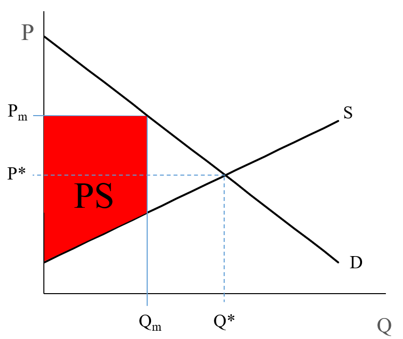
(Note: in Figure 5.2, I use and to represent “monopoly equilibrium quantity” and “monopoly equilibrium price.")
At which value of is the producer surplus (the profit, the red area) the largest?
Answer: it is maximized when supply = MC = MR (Marginal Revenue).
What is marginal revenue? Well, it is the amount of money a firm takes in from selling one more unit of the good. If the price is constant, then MR = price - selling one more unit means we collect one more times the price. But, in this case, since the monopolist faces a downward sloping demand curve, each additional unit he sells will have a lower price, and he will sell every unit at that lower price. As an example, using the demand curve in the previous numerical example, if the monopolist sets , then he sells 50 units at a price of 500, and has total revenue of 500 x 50 = 25,000. If he makes one more unit, he sells 51 units at a price of 492 (price is derived from the demand curve, 900-8*51=492), for a revenue of 25,095. His marginal revenue from making one more unit is 95, even though the price is 492.
So, we need to plot the marginal revenue curve.
It turns out that the marginal revenue curve is a line that has the same y-intercept as the demand curve, but has a slope that is twice as steep. So, for example, if our demand curve is given as , then 100 is the intercept and -1 is the slope (remember the equation of a line; . In our case, , which is another way of writing .
So, the marginal revenue curve has the same intercept, 100, but is twice as steep, with a slope of -2.
This is written as:
An Aside...
Here is a small aside, which is not obligatory and not something you will be quizzed on. If you know calculus, you will be able to understand the following calculus-based explanation of why the monopolist sets his quantity to be that where MR = MC, and how we derive .
A monopolist wants to maximize profit, and profit = total revenue - total costs.
We can write this as . In calculus, to find a maximum, we take the first derivative and set it to zero:
Profit is maximized when
= marginal revenue and = marginal cost
So, is the same as , which is the same as MR = MC.
To find MR: .
If the demand curve is given by then
So,
So, the MR curve has the same intercept as the demand curve, but its slope is exactly double that of the demand curve.
Generally, if a Demand curve is given as , then .
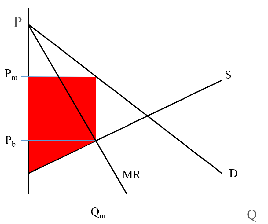
In Figure 5.3, the MR curve is shown in blue. To find the profit maximizing point, set to the amount where the MR and MC curves intersect. These will be sold at price . Any other quantity will give a smaller profit (the red area on the graph).
So, it is important to remember two things:
- The marginal revenue (MR) is a line with the same intercept as the demand curve, but with a slope twice as steep; and
- When , profit is maximized.
We say that in a monopoly, profit is maximized when , just like in a competitive market, when MR = Price = MC. You will remember that in a competitive market, the demand curve is flat. Its slope is zero. So, the derivative of this curve, which is the MR curve, also has a slope of zero (two times zero = zero). So the result that P(max) occurs when MR = MC is true not just in a monopoly, but all markets.
Example
The demand curve is given as: .
The supply curve is given as: .
- What is the profit-maximizing (monopoly) equilibrium?
- Find the Consumer Surplus and Producer Surplus
- What is the dead-weight loss?
Answers:
-
In order to answer this question, first, we need to find the monopoly equilibrium. To do so, first, we have to solve the MR = MC for the Q. MC is the supply function, and we learned that if demand curve is given as , then
So, MR equation will be .And will be set by the demand curve:
-
Consumer surplus equals the area of the under the demand curve and monopoly price , horizontal line.
Coordinates of three corners of this triangle will be:
Top left: (0, demand curve intercept) = (0, 140)
Bottom left:
Right corner:Producer surplus equals the area of the under the monopoly price and above the supply curve (red area), which equals the area of the trapezoid.
Coordinates of four corners of this trapezoid are:
Top left: (0, Pm) = (0, 100)
Bottom left: (0, supply curve intercept) = (0, 20)
Top right:
Bottom right:Note that coordinate of bottom right corner of the trapezoid (MR and supply curve intersection) can be found by plugging the Qm in the supply curve,
And the area of the trapezoid will be:
-
The dead-weight loss is the triangle between the demand and supply curves (competitive market equilibrium) and the vertical line Qm. So, first, we need to find the competitive market equilibrium:
Demand curve: .
Supply curve: .At the competitive market equilibrium: demand = supply
140 – 2Q = 20 + 2Q
Q* = 30
P* = 140 – 2*30 = 80Coordinates of three corners of this triangle will be:
Top left: , which is (20, 100)
Bottom left: = (20, 60)
Right: = (30, 80)Now that we have the coordinates of three corners, we should be able to find the area of the triangle as:
Dead-weight loss
Note that dead-weight loss can also be calculated by deducting the monopoly market total wealth (CS + PS) from competitive market total wealth.
Your turn!
Practice Exercise
Assume In a hypothetical market demand and supply functions for a good are
Demand:
Supply:
- Calculate the competitive market equilibrium, consumer surplus, producer surplus, and total wealth created by the market.
- Calculate the monopoly Price and quantity, consumer surplus, producer surplus, and total wealth.
- Caclulate the dead-weight loss of the monopoly.
Calculate the dead-weight loss using this method and compare your answer with what we calculated. You should have similar results.
Try and work it through and see if you can get these answers.
Take Aways
After this lesson and the associated readings, you should be able to:
- define and understand the meaning of “market power;”
- know the names of markets with:
- one seller,
- two sellers,
- a few sellers,
- one buyer;
- understand why a monopolist can set price or quantity, but not both;
- describe the three ways a monopoly can come into existence;
- explain the effects of a monopoly on price and quantity compared to a free market;
- understand what happens to consumer and producer surplus in a monopoly;
- understand the concept of a “dead-weight loss” and a “social cost;”
- understand and apply the rule for profit maximization in a monopoly;
- find the marginal revenue curve:
- the intercept of the marginal revenue curve,
- the slope of the marginal revenue curve;
- find the monopoly equilibrium and compare it to the competitive equilibrium.