
Decision Analysis Without Probabilities: Sensitivity, Threshold and Scenario Analysis
In the oil-field example from the previous section, the probabilities of a dry hole and a producer were known with confidence. This isn’t always true in the real world. Moreover, sometimes in real-world situations, there are so many possible outcomes that is impossible to assign a specific probability to each outcome. Suppose, just hypothetically, that oil prices could vary between $50 and $100 per barrel over the next five years. What is the probability that oil prices will average $50.03 per barrel? $50.04 per barrel? $99.30 per barrel?
In cases where determining probabilities explicitly is not possible or practical, threshold analysis and sensitivity analysis can be useful in understanding how the net present value of different alternatives may vary with some variation in key variables. Both of these techniques are useful in identifying situations under which one alternative is better than another. This can make even complex decision problems much more tractable for the decision-maker, since it reduces the problem from needing to calculate net present values for a large number of alternative outcomes to a judgment of whether one or another set of outcomes is more likely.
As we go through these techniques, we will often refer to something called a “parameter” in the decision problem. In this case, a parameter refers to a variable whose value affects the outcome of one or more alternatives – so a parameter is different from an alternative. In the oil field problem, the major parameter would be whether the field is a dry hole or whether it is a producer (so the parameter itself would be the probability of a producer versus a dry hole). The price of oil or the quantity of oil (if any) might be other important parameters for a problem such as this one.
Sensitivity Analysis
Sensitivity analysis proceeds by selecting one parameter, changing its values, and observing how these new values change the net present value (or EMV) of some alternative. If sensitivity analysis is conducted using a small range of alternative values, or if the alternative values represent different scenarios, then it is sometimes (aptly) called “scenario analysis.” There's more material on scenario analysis further down this page.
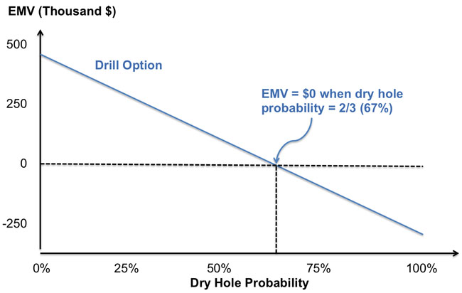
We’ll illustrate this using the oil-field problem, performing a sensitivity analysis on the EMV of the drilling option as we vary the dry-hole probability. In this case the outcome is the EMV and the parameter that we are varying is the probability of a dry hole. This analysis is pretty straightforward since we can write an expression for the EMV of drilling. We will need to use the fact that P(producer) = 1 – P(dry hole). (What rules of probability tell us that this is true?)
We can rearrange terms in the equation to get:
This equation tells us a couple of things. First, the EMV of drilling is going to decline as the probability of a dry hole increases. This makes sense, since we lose money if we drill ourselves and the field is not a producer. Second, the relationship between EMV and the dry hole probability is linear, so the EMV falls at a constant rate as the dry hole probability increases. We can also use the equation to find the dry hole probability where the EMV is equal to zero. We do this by setting EMV(drill) equal to zero and manipulating the equation as follows:
Normally, sensitivity analysis is utilized to visualize the change in net present value or EMV with the change in some parameter of interest. For the drilling option, this is shown in Figure 10.2, which plots the EMV versus the dry hole probability. Also shown in Figure 6.2 is the dry-hole probability where the EMV is equal to zero.
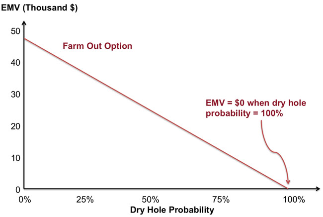
As an exercise for yourself, perform the same sensitivity analysis on the option to farm-out. The parameter is still the same (the probability of a dry hole) but the outcome is different (the option to farm-out versus the option to drill). Your graph should look like the one in Figure 6.3.
Threshold Analysis
Threshold analysis (also called break-point analysis) seeks to identify the value of a parameter where the best decision changes. Instead of asking what the probability of a producer versus a dry hole might be (and what are the associated EMVs of the option to drill or farm-out), a threshold analysis would ask how likely would it need to be for the field to be a producer for the expected-value decision-maker to choose the option to drill.
Threshold analyses can proceed graphically or algebraically. We will use the oil field example to illustrate both. Remember that the EMV of both the drilling and the farm-out options are functions of the dry-hole probability and of the NPVs for drilling and farming-out. Holding the NPVs constant as in Table 10.1, we can write a mathematical expression for the EMV of each option as a function of the dry-hole probability P(dry hole). We will need to use the fact that P(producer) = 1 – P(dry hole). (What rules of probability tell us that this is true?)
If we graph the EMVs together on the same set of axes (as in Figures 6.2 and 6.3), the point at which the two lines cross would be the threshold. Figure 6.4 illustrates this crossing point. Note that the scale of the axes, especially the horizontal axis, is different than in Figures 6.2 or 6.3.
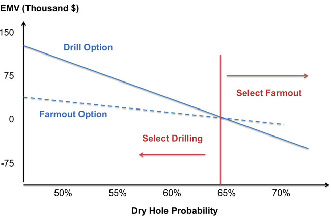
Looking carefully at Figure 6.4, we can see that at a dry hole probability of around 65% or lower, the EMV of drilling is higher than the EMV of the farm-out option (this is why the drilling curve is above the farm-out curve). If the dry hole probability is above 65%, then the farm-out option has a higher EMV.
Algebraically, we can solve explicitly for the threshold value of the dry hole probability, by setting EMV(drill) equal to EMV(farm-out) and solving for the dry hole probability that makes these EMVs identical. Here we go!
Threshold analysis in particular can be a very powerful way of making difficult decisions seem more tractable. Even in the simple oil-field problem, the relevant question for the investor evaluating the oil-field decision is not to determine the exact probability of the field being a producer. The threshold analysis approach asks the potential investor whether they believe that there is more than a 65% chance of the field being dry. If so, then they should farm out drilling or not drill at all. If not, then the investor should choose to drill themselves.
Scenario Analysis
Scenarios about future outcomes or states of the world can be powerful tools for getting decision-makers to think about uncertainty. While scenario analysis is simpler than a sensitivity or a threshold analysis, scenarios can often be made up of specific values of multiple parameters. Scenario analysis is not about predicting the future or making projections. Like sensitivity and threshold analysis, it is a way to get decision-makers to consider different possible future states of the world, to identify the drivers that might lead to those states of the world, and to make plans for those possible states of the world.
In the energy world, one of the pioneers of scenario-based planning has been Shell, which started using scenario-based planning in the 1960s, as computer-aided decision-making was emerging among large businesses. Shell adopted scenario planning when it (and other large energy companies) were surprised by the emergence of environmentalism and the OPEC cartel as unforeseen but potentially disruptive forces to their business. The Harvard Business Review has a nice article about Shell's development and use of scenario planning. (The article is also available through Canvas.)
The process of scenario planning has a number of steps:
- Determine drivers of change (largely done via brainstorming)
- Determine links and interdependencies among drivers of change - an example is that technological and regulatory change may be intertwined. The purpose of this step is to recognize the existence of interdependent or connected drivers of change, and possible directions of influence.
- Group drivers that are logically connected into "scenarios." Typically, at this stage the scenarios are brainstormed, without too much worry about whether the scenarios overlap with or contradict one another.
- The larger set of scenarios is reduced to a smaller set of scenarios. In Shell's method, the aim is to get to around three scenarios - the idea is that this avoids a focus on one scenario as being the most or least likely. It's also important to recognize at this stage that scenarios are different than alternatives so we don't really talk about scenarios that might be preferred over others. At this stage, scenarios are ideally complementary rather than in opposition (having a good and bad scenario, for example).
- Tell a story about each scenario. This often involves giving each scenario a name and including some context - not just the specific parameter values associated with different scenarios but the events that might lead to those scenarios.
Scenario planning has its critics - one thing about scenarios, for example, is that good scenarios are based around plausibility and not probability. This can lead to different decision-makers having different views of likely versus unlikely states of the world. Regardless, scenario planning is still a widely-used tool for decision-making.