Regional Transmission Organizations
Regional Transmission Organizations (RTOs) are non-profit, public-benefit corporations that were created as a part of electricity restructuring in the United States, beginning in the 1990s. Some RTOs, such as PJM in the Mid-Atlantic states, were created from existing “power pools” dating back many decades (PJM was first organized in the 1920s). The history of the RTO dates back to FERC Orders 888 and 889, which suggested the concept of the “Independent System Operator” (ISO) to ensure non-discriminatory access to transmission systems. FERC Order 2000 encouraged, but did not quite require, all transmission-owning entities to form or join a Regional Transmission Organization to promote the regional administration of high-voltage transmission systems. The difference between RTO and ISO is, at this point, largely semantic. Order 2000 contains a set of technical requirements for any system operator to be considered a FERC-approved RTO.
RTOs are regulated by FERC, not by the states (i.e., RTO rules are determined by a FERC-approved tariff and not by state Public Utility Commissions) and membership in a RTO by any entity is voluntary. Including Texas (which is technically outside of FERC’s jurisdiction), there are seven RTOs in the U.S., covering about half of the states and roughly two-thirds of total U.S. annual electricity demand. Each RTO establishes its own rules and market structures, but there are many commonalities. Broadly, the RTO performs the following functions:
- management of the bulk power transmission system within its footprint;
- ensuring non-discriminatory access to the transmission grid by customers and suppliers;
- dispatch of generation assets within its footprint to keep supply and demand in balance;
- regional planning for generation and transmission (though see below for limitations to this function);
- with the exception of the Southwest Power Pool (SPP), RTOs also run a number of markets for electric generation service.
In many ways, RTOs perform the same functions as the vertically-integrated utilities that were supplanted by electricity restructuring. There are, however, a number of important distinctions between RTOs and utilities.
- RTOs do not sell electricity to retail customers. RTOs purchase power from generators, resell it to electric distribution utilities, who then resell it again to end-use customers.
- RTOs may not earn profits.
- RTOs do not own any physical assets – they do not own generators, power lines or any other equipment. RTOs generally cannot force generation or transmission companies to make investments.
- RTO decision-making is governed by a “stakeholder board” consisting of various electric sector constituencies. In some cases, the RTO can implement policy unilaterally without approval by the stakeholder board, but this is generally rare. All policies must, however, be approved by FERC.
- RTOs do not take any financial or physical position in the markets they operate. They must remain neutral market-makers, although they do monitor activity in their markets to avoid manipulation by individual generators or groups of generators.
The set of NETL power market primers zipped file contains more information on specific differences between the various RTO markets.
The separation of ownership from control in RTO markets raises some interesting complications for planning. RTOs have responsibility for ensuring reliability and adequacy of the power grid. They must perform regional planning, meaning that they determine where additional power lines and generators are required in order to maintain system reliability. But RTOs generally cannot require that member companies make any investments. They generally rely on a variety of market mechanisms to create financial incentives for member firms to invest in generation. Many transmission investments needed for reliability are eligible for fixed rates of return set by FERC.
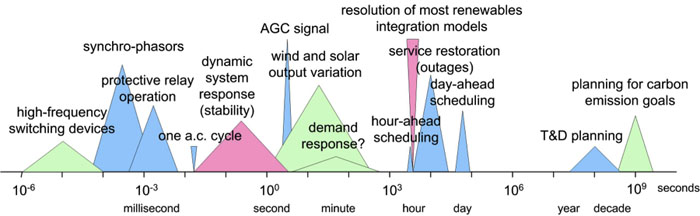
Operating a power system requires making decisions on time scales covering fifteen orders of magnitude prior to real-time dispatch, as shown in Figure 11.5.
Since the RTO does not own any physical assets, it must effectively sign contracts with generation suppliers to provide needed services. The market mechanisms run by the RTO are used to procure generation supplies needed to maintain reliability. Once generation supplies are procured by the RTO, it can dispatch generation as needed to meet demand.
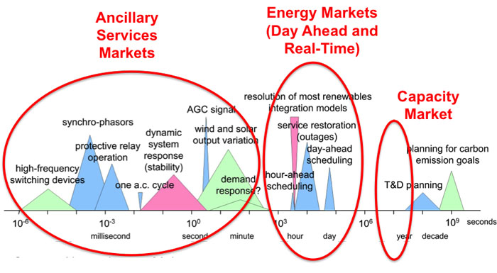
RTOs run three types of markets that enable them to manage the power grid over time scales ranging from cycles (one cycle = 1/60th of one second) to several years in advance of real-time dispatch, as shown in Figure 11.6.
Capacity Markets are meant to provide financial incentives for suppliers to keep generation assets online and to induce new investment in generation. Capacity markets are generally forward markets to have generation capacity online and ready to produce electricity at least one year ahead of time. PJM’s capacity market is run three years ahead of time. For example, a generator that participates in the PJM capacity market in 2023 is effectively making a promise to have generation capacity online and ready to produce in 2026. Capacity markets are thought to be necessary because prices in other RTO markets are not always sufficiently high to keep existing generation from shutting down or to entice new generators to enter the market. Not all RTOs have forward capacity markets. Texas, for example, does not operate a capacity market. We will discuss capacity markets in more detail in Lesson 12.
Energy Markets are perhaps the most well-known of all market constructs run by RTOs. Like capacity markets, energy markets are forward markets but are used by the RTO to ensure that enough generation capacity is online and able to produce energy on a day-ahead (24-hour ahead) to one-hour-ahead basis. RTOs run two types of energy markets. The first, the “day-ahead market” is used to determine which generators are scheduled to operate during each hour of the following day (and at what level of output), based on a projection of electricity demand the following day. The second, the “real-time market” is somewhat poorly named; this market is used by the RTO to adjust which generators are scheduled to run on an hour-ahead basis. A better term for the real-time market (which is used in some cases) would be “adjustment market” or “balancing market” since supplies for this so-called real-time market are actually procured one day in advance (but after supplies are procured through the day-ahead market). The prices prevailing in the day-ahead and real-time markets are the most commonly referenced and quoted of all markets run by the RTOs.
Ancillary Services Markets allow the RTO to maintain a portfolio of backup generation in case of unexpectedly high demand or if contingencies, such as generator outages, arise on the system. There are many different types of ancillary services, corresponding to the speed with which the backup generation needs to be dispatched. “Reserves” represent capacity that can be synchronized with the grid and brought to some operating level within 60, 30, or 15 minutes. “Regulation” represents capacity that can change its level of output within a few seconds in response to fluctuations in the system frequency. Ancillary services are increasingly important for renewable energy integration, so we will discuss those markets in Lesson 12.
Suppliers may participate in multiple markets. For example, a 100 MW generator could offer 80 MW to the day-ahead market, 10 MW to the real-time market, and 5 MW each to the regulation and reserves markets. The generator would earn different payments for each type of service provided to the grid. Thus, while the day-ahead or real-time price is often referred to as “the” market price of electricity, in reality, there are many different prices in the RTO market at any given time, each representing a different type of service offered to the RTO.
Because the RTO operates its entire system in an integrated way, even though its footprint may encompass many different utility territories and transmission owners, RTO type markets are sometimes referred to as “power pools” or simply “pools.” The following video contains more information about how the pool-type markets are structured, using the largest pool type model (PJM, in the Mid-Atlantic U.S.).
Video: PJM Model and SMP (9:37)
Seth Blumsack: PJM - ah, they used a different model, a different market model, which is sometimes called a pool. And the way the PJM, or pool market, works is that individual generators commit their capacity to the market, or the pool. The pool decides which generators are going to run at which hours. The way that generators are allowed to structure supply offers is much more limited in the pool than it was in the power exchange. In the pool, the supply offers from generators basically just reflected variable cost. And so, capital cost recovery and other things were made up through separate payments or separate markets.
So, the pool-type market has really become the dominant market model used in the US today. The pool-type market was, more or less, what FERC's standard market design looked like. The markets that are run by regional transmission organizations are all run as what we call uniform price auctions. They way that a uniform price auction works is that suppliers submit supply offers to the RTO and then these offers are aggregated to form a system supply curve. Originally, demand was assumed to be perfectly inelastic - which is the same thing as saying a vertical demand curve - so, whatever demand happened to be, that's what it was and they would pay whatever price the market happened to produce. At the point where this vertical demand curve crossed the offer curve, or the supply curve, was the market clearing price, or what we call the system marginal price for that particular time. I'll show you a couple of different pictures of this.
This is approximately what the supply curve looks like for the PJM market. A couple of things about this supply curve are that, first of all, it has this hockey stick sort of shape. Over a large range of electricity demand, the market price would not vary all that much - or the cost of generation would not vary all that much. In the example that I have here, if demand is a hundred thousand megawatt hours, which is this vertical line about here, then the point where that line crosses the supply curve is what sets the market price for that particular time period. And so, in this particular time period, at a demand of a hundred thousand megawatt hours, the price would be eighty dollars per megawatt hour. And if the price were a little bit lower or a little bit higher than that, say eighty thousand instead of a hundred thousand, the market clearing price would not change all that much. But as demand increases, in this case past a hundred and or a hundred and twenty thousand megawatt hours, then the cost of the capacity you'd have to use in order to satisfy that demand starts to rise very sharply. So, this point, the part of the supply curve over here where the price starts to rise very steeply is sometimes called the "devil's elbow."
If we have demand of a hundred and forty thousand megawatt hours, then, all of a sudden, the price would jump to $160 per megawatt hour. So, we have increased demand by 40% and we have doubled the price. At high levels of electricity demand, the small changes in demand can produce much larger than proportional changes in the market price.
The last generator that is dispatched to meet electricity demand is the generator that basically sets the market price, or the system marginal price. And the way these uniform price auctions work is that that system marginal price, or that market price, is paid to every generator whose supply offer was lower than the market price. So, if you're a generator, your profit during any time period is equal to whatever the market the price is minus your marginal cost. Sometimes, you'll hear this market referred to as a scarcity rent. The way that these uniform price auctions work, if you've take Econ 101, is not dissimilar to just about any other market in the world.
There is a variation on the uniform price auction called the pay-as-bid auction. This is used in the UK but not in the United States. The idea behind the pay-as-bid auction is that there's still a system marginal price that is produced through the market, but rather than each generator earning the system marginal price, each generator who is accepted into the auction, each generator that bids below what the system marginal price turns out to be, is payed whatever their bid was. As I said, this is used in the UK but not in the US. The belief in the US is that if you switched to a pay-as-bid system, this would simply give generators incentives to manipulate their bids. So, if you're a generator that has a marginal cost of five dollars per megawatt hour and you believe that the market price, or the system marginal price, will be fifty dollars per megawatt hour, in the uniform clearing price option, you would earn fifty minus five equals forty-five dollars per megawatt hour in profit. In the pay-as-bid auction, if you actually submitted a bid that was equal to your marginal cost, then you would earn five dollars per megawatt hour. The thought is, in the US, is that this would give this particular supplier an incentive to inflate their bid up to whatever they thought the market clearing price would be. So, the pay-as-bid is not really used in the US.
So, basically, all of the centralized wholesale markets run by RTOs follow this uniform price option format.
If you are interested, the following two videos discuss electricity market structures that are alternatives to the pool:
Video: Bilateral Markets Exist in Regions of the U.S. (4:25)
Seth Blumsack: Areas of the US that do not have these centralized electricity markets do have wholesale trade of electricity between generators and buyers, between utilities and so on and so forth. These are what we call bilateral markets, and these bilateral markets actually existed long before electricity deregulation, long before the PJM electricity market and so on and so forth. The first of these was actually set up in the western US in the late 1980s. It was called the Western Systems Power Pool. It's actually still in place - so, the market structure that was set up in the 1980s in the western states is actually still used there today.
The way that bilateral markets work is that large volumes of electricity, sometimes called bulk power, is traded between utilities, between buyers and sellers, at whatever price the two counter parties agree upon. And how these trades actually occur is that potential counter parties actually call each other up on the phone. So, I might be, like, Bonneville Power Administration and I could call somebody at SMUD (The Sacramento Municipal Utility District) and say, "I've got spare electricity to sell; do you want to buy any?" This is basically how the bilateral markets work. And sometimes, the energy that's purchased through these bilateral markets is coupled with access to the transmission grid so that you could actually deliver the electricity. This is sometimes called "firm" energy, as opposed to non-"firm" energy, which is sold without access to the transmission grid. These bilateral markets still exist today. Now, a lot of the bilateral trading takes place over electronic trading platforms. People don't call each other up on the phone as much; instead they might log in to some electronic trading platform, kind of like e-Bay or something like that. When we talk about centralized electricity markets, just keep in mind that places in the US that do not have centralized electricity markets still have trading of electricity through these bilateral markets.
In the mid-1990s, California and a handful of Mid-Atlantic states (the "PJM" market, which stands for Pennsylvania, New Jersey, and Maryland), as part of a broader electricity market restructuring effort, set up much more coordinated, much more formal mechanisms for trading electricity. The California model was a little bit different from the PJM model, but the big similarity that they shared was that rather than people calling each other up on the phone, there would be a centralized exchange setup, kind of like something analogous to the New York Stock Exchange or the New York Mercantile Exchange, where crude oil futures are traded. And rather than buyers and sellers trying to find each other by calling each other up on the phone, everybody would go to this centralized market, or this centralized exchange
Video: The Power Exchange Model Was Tried for a Couple of Years in California (6:00)
Seth Blumsack: Video 11.3: The power exchange model was tried for a couple of years in California, prior to that state’s energy crisis in 2000 and 2001. The function of the power exchange is to facilitate the purchase and sale of bulk wholesale electricity using a structure very much like a financial exchange.
Click for transcript of The Power Exchange Model Was Tried for a Couple of Years in California.
For these centralized electricity markets….I'd said that starting in the 1990s there were two competing models for setting up electricity markets: one in California and one in the PJM states. What California did was it tried most directly to replicate a financial exchange, like the New York Stock Exchange, for buying and selling electricity. And so, it opened The California Power Exchange. So, California's biggest utilities, they all agreed to go along with this, and they agreed to buy all of their power from the power exchange. So, how the power exchange worked was this:
First, individual generators decided whether or not they wanted to enter their supplies into the power exchange. This is called decentralized unit commitment. It was up to the generators whether or not they wanted to make their capacity available to the exchange. The bids from the generators, there was an overall cap, so a maximum amount, that the generators could bid, but beyond that, the generators could more or less do whatever they wanted. They could submit whatever type of supply offer they wanted to. And then, just as generators had to submit supply offers, the three large California utilities, they also had to submit demand bids. So, the idea was that you would have so many suppliers rushing into this market to serve so much electricity demand that there would be sort of this vigorous competition that would ensue, sort of like in an auction.
So, the way that the power exchange market worked was that every hour, suppliers would submit supply offers, which is the blue curve here, and the supply offer indicated how much generating capacity the supplier was willing to make available to the power exchange at what price. So, when you put all of these together you got what we call a supply curve or an offer curve. And that's in the blue. On the demand side, the utilities had to submit the amount of electricity that they were willing to buy from the exchange at some price. And so, that's the pink curve right over here. And when these purchase offers were aggregated together you got kind of a California system demand curve. And where the supply and demand curve met determined the price and quantity at which the electricity market would clear. So, in this example, and this is a picture from the late 1990s, the point where supply equals demand, the market cleared for this particular hour at about 32,500 megawatts of generation capacity would be utilized to serve 32,500 megawatt hours of energy demand, and the market clearing price would be $190 per megawatt hour. So, this was repeated every single hour of every single day. And in the event that there wasn't enough electricity purchased in through the power exchange to serve all of California's electricity demand, there was a secondary balancing market that would ultimately equate demand and supply on a sub-hourly basis. So, this was basically how the power exchange model worked, and the California power exchange lasted for about two and a half years, and after the California power crisis, as California's sort of screeching halt to electricity deregulation, the power exchange was shut down. Partially because of California's sort of dismal failure, the power exchange model has not really been replicated anywhere else except in Alberta, up in Canada, where they actually have had a power exchange type market for well over a decade. They seem to like it, but in California, it didn't work so well.
Virtually all RTO markets are operated as “uniform price auctions.” Under the uniform price auction, generators submit supply offers to the RTO, and the RTO chooses the lowest-cost supply offers until supply is equal to the RTO’s demand. This process is called “clearing the market.” The last generator dispatched is called the “marginal unit” and sets the market price. Any generator whose supply offer is below the market-clearing price is said to have “cleared the market,” and is paid the market-clearing price for the amount of supply that cleared the market. Generators with marginal operating costs below the market-clearing price will earn profits. In general, if the market is competitive (all suppliers offer at marginal operating cost) the marginal unit does not earn any profit.
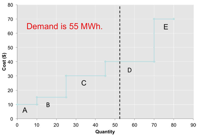
The uniform price auction is illustrated in Figure 11.7. There are five suppliers, each of which offers its capacity to the market at a different price. These supply offers are shown in Table 11.1. Here we will assume that supply offers are equal to the marginal costs of each generator, but in the deregulated generation market suppliers are not really obligated to submit offers that are equal to costs. The RTO aggregates these supply offers to form a single market-wide “dispatch stack” or supply curve. Demand is represented by a vertical line (the RTO assumes that demand is fixed, or “perfectly inelastic” with respect to price). In this case, demand is 55 MWh. Generators A, B, C and D clear the market. Generator E does not clear the market since its supply offer is too high. The market-clearing price, known as the “system marginal price (SMP)” would be $40 per MWh. Generators A, B, C, and D would each be paid $40 per MWh. Generators A, B and C would earn profit. Generator D is the marginal unit so it earns zero profit.
| Supplier | Capacity (MW) |
Marginal Cost ($/MWh) |
|---|---|---|
| A | 10 | $10 |
| B | 15 | $15 |
| C | 20 | $30 |
| D | 25 | $40 |
| E | 10 | $70 |
Let’s calculate the profits for each of our generators. Remember that each generator that clears the market (in this case, it would be A, B, C, and D; E does not clear the market) earns the SMP for each unit of electricity they sell. Total profits are thus calculated as:
Profit = Output × (SMP – Marginal Cost).
Since the SMP in our example is equal to $40, profits are calculated as:
Firm A profit = 10 × (40 – 10) = $300
Firm B profit = 15 × (40 – 15) = $375
Firm C profit = 20 × (40 – 30) = $200
Firm D profit = 10 × (40 – 40) = $0
Firm E profit = 0 × (40 – 70) = $0.
Note in particular that Firm D, which is the “marginal unit” setting the SMP of $40/MWh, clears the market but does not earn any profits. We will come back to this case when we discuss capacity markets in Lesson 7.