2.2 The Need for Coordinate Systems

Figure 2.2. A Cartesian coordinate system.

Credit: © Penn State University, is licensed under CC BY-NC-SA 4.0

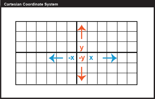
Locations on the Earth's surface are measured and represented in terms of coordinates; a coordinate is a set of two or more numbers that specifies the position of a point, line, or other geometric figure in relation to some reference system. The simplest system of this kind is a Cartesian coordinate system, named for the 17th century mathematician and philosopher René Descartes. A Cartesian coordinate system, like the one above in Figure 2.2, is simply a grid formed by put together two measurement scales, one horizontal (x) and one vertical (y). The point at which both x and y equal zero is called the origin of the coordinate system. In the illustration above, the origin (0,0) is located at the center of the grid (the intersection of the two bold lines). All other positions are specified relative to the origin. The coordinate of the upper right-hand corner of the grid is (6,3). The lower left-hand corner is (-6,-3).

Figure 2.3. The geographic (or "geodetic") coordinate system.

Credit: © Penn State University, is licensed under CC BY-NC-SA 4.0

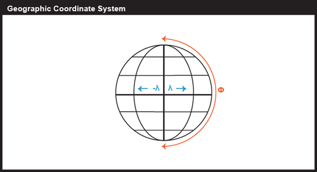
Cartesian and other two-dimensional (plane) coordinate systems are handy due to their simplicity. They are not perfectly suited to specifying geographic positions. However, the geographic coordinate system, as seen in Figure 2.3, is designed specifically to define positions on the Earth's roughly spherical surface. Instead of the two linear measurement scales x and y, the geographic coordinate systems bring together two curved measurement scales.

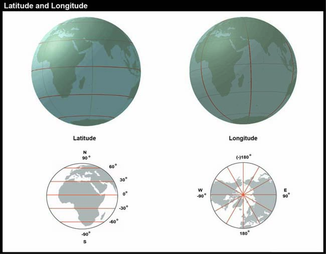
You have probably encountered the terms latitude and longitude before in your studies. A comparison of these two scales is given below in Figure 2.4. The north-south scale, called latitude (designated by the Greek symbol phi), ranges from +90° (or 90° N) at the North pole to -90° (or 90° S) at the South pole while the equator is 0°. A line of latitude is also known as a parallel.

The east-west scale, called longitude (conventionally designated by the Greek symbol lambda), ranges from +180° to -180°. Because the Earth is round, +180° (or 180° E) and -180° (or 180° W) are the same grid line. A line of longitude is called a meridian. That +/- 180 grid line is roughly the International Date Line, which has diversions that pass around some territories and island groups so that they do not need to cope with the confusion of nearby places being in two different days. Opposite the International Date Line on the other side of the globe is the prime meridian, the line of longitude defined by international treaty as 0°. At higher latitudes, the length of parallels decreases to zero at 90° North and South. Lines of longitude are not parallel, but converge toward the poles. Thus, while a degree of longitude at the equator is equal to a distance of about 111 kilometers, that distance decreases to zero at the poles.

Figure 2.4.The geographic coordinate system.

Credit: Raechel Bianchetti © Penn State University, is licensed under CC BY-NC-SA 4.0

2.2.1 Geographic Coordinates

We have discussed the fact that both latitude and longitude are measured in degrees, but what about when we need a finer granularity measurement? To record geographic coordinates, we can further divide degrees into minutes, and seconds. The degree is equal to sixty minutes, and each minute equal to sixty seconds. Geographic coordinates often need to be converted in order to geo-register one data layer onto another. Geographic coordinates may be expressed in decimal degrees, or in degrees, minutes, and seconds. Sometimes, you need to convert from one form to another.

Here's how it works:

To convert Latitude of -89.40062 from decimal degrees to degrees, minutes, seconds:

Subtract the number of whole degrees (89°) from the total (89.40062°). (The minus sign is used in the decimal degree format only to indicate that the value is a west longitude or a south latitude.) In this example, the minus sign indicates South, so keep track of that.

Multiply the remainder by 60 minutes (.40062 x 60 = 24.0372).

Subtract the number of whole minutes (24') from the product.

Multiply the remainder by 60 seconds (.0372 x 60 = 2.232). Round off (to the nearest second in this case).

Assemble the pieces; the result is 89° 24' 2" S. If the starting point had been the Longitude of -89.400062, the only difference would be that the S above would be replaced by a W.

To convert 43° 4' 31" from degrees, minutes, seconds to decimal degrees, use the simple formula below:
DD = Degrees + (Minutes/60) + (Seconds/3600)

Divide the number of seconds by 60 (31 ÷ 60 = 0.5166).

Add the quotient of step (1) to the whole number of minutes (4 + 0.5166).

Divide the result of step (2) by 60 (4.5166 ÷ 60 = 0.0753).

Add the quotient of step (3) to the number of whole number degrees (43 + 0.0753).

The result is 43.0753°

2.2.2 Plane Coordinates

So far, you have read about Cartesian Coordinate Systems, but that is not the only kind of 2D coordinate system. A plane coordinate system can be thought of as the juxtaposition of any two measurement scales. In other words, if you were to place two rulers at right angles, such that the "0" marks of the rulers aligned, you would define a plane coordinate system. The rulers are called "axes." Just as in Cartesian Coordinates, the absolute location of any point in the space in the plane coordinate system is defined in terms of distance measurements along the x (east-west) and y (north-south) axes. A position defined by the coordinates (1,1) is located one unit to the right, and one unit up from the origin (0,0). The Universal Transverse Mercator (UTM) grid is a widely-used type of geographic plane coordinate system in which positions are specified as eastings (distances, in meters, east of an origin) and northings (distances north of the origin).

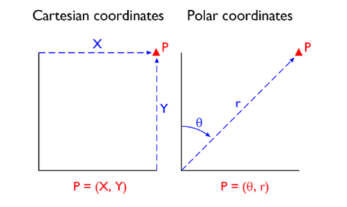
Some coordinate transformations are simple. The transformation from non-georeferenced plane coordinates to non-georeferenced polar coordinates, described in further detail later in the chapter, shown below involves nothing more than the replacement of one kind of coordinates with another.

Figure 2.5. The same position specified within two non-georeferenced plane coordinate systems: Cartesian (left) and polar (right).

Credit: from Scales and Transformations by David DiBiase, and licensed under CC BY-NC-SA 4.0

2.2.3 UTM: Universal Transverse Mercator

Figure 2.6. The ten UTM zones that span the conterminous U.S.

Credit: U.S. Geological Survey, public domain, 2004

The geographic coordinate system grid of latitudes and longitudes consists of two curved measurement scales to fit the nearly-spherical shape of the Earth. As discussed above, geographic coordinates can be specified in degrees, minutes, and seconds of arc. Curved grids are inconvenient to use for plotting positions on flat maps. Furthermore, calculating distances, directions, and areas with spherical coordinates is cumbersome in comparison to doing so with plane coordinates. For these reasons, cartographers and military officials in Europe and the U.S. developed the UTM coordinate system. UTM grids are now standard not only on printed topographic maps but also for the geographic referencing of the digital data that comprise the emerging U.S. "National Map" (NationalMap.gov).

"Transverse Mercator" refers to the manner in which geographic coordinates are transformed from a spherical model of the Earth into plane coordinates. The act of mathematically transforming geographic spherical coordinates to plane coordinates necessarily displaces most (but not all) of the transformed coordinates to some extent. Because of this, map scale varies within projected (plane) UTM coordinate system grids. Thus, UTM coordinates provide locations specifications that are precise, but have known amounts of positional error depending on where the place is.

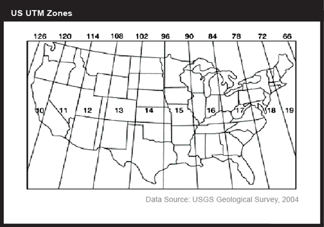
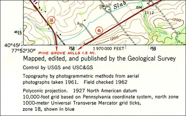
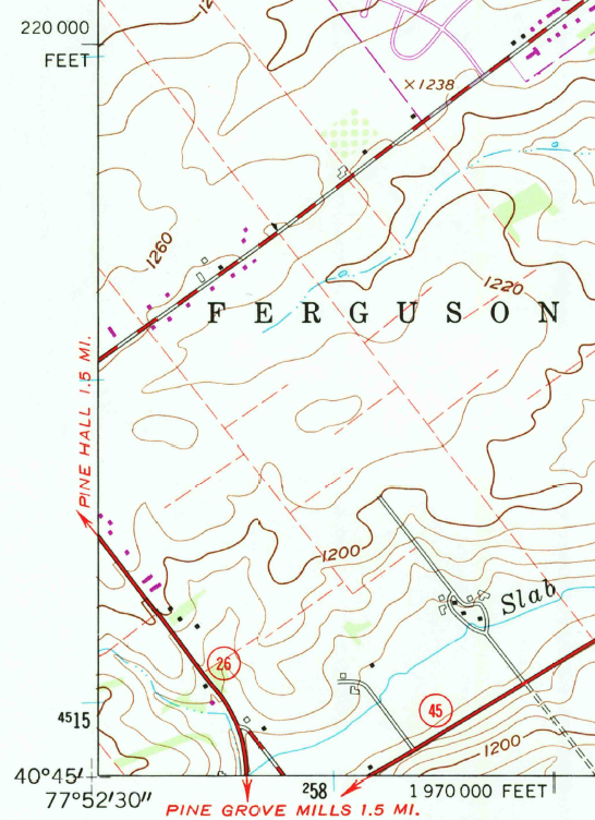
Shown below is the southwest corner of a 1:24,000-scale (for which 1 inch on the map represents 2000 ft. in the world) State College topographic map in Centre County, PA, published by the United States Geological Survey (USGS). Note that the geographic coordinates (40° 45' N latitude, 77° 52' 30" W longitude) of the corner are specified. Also shown, however, are ticks and labels representing two plane coordinate systems, the Universal Transverse Mercator (UTM) system and the State Plane Coordinates (SPC) system. The tick on the west edge of the map labeled "4515" represents a UTM grid line (called a "northing") that runs parallel to, and 4,515,000 meters north of, the equator. Ticks labeled "258" and "259" represent grid lines that run perpendicular to the equator and 258,000 meters and 259,000 meters east, respectively, of the origin of the UTM Zone 18 North grid (see its location on Fig 6 above). Unlike longitude lines, UTM "eastings" are straight and do not converge upon the Earth's poles.

Figure 2.7. Southwest corner of a USGS topographic map showing grid ticks and labels for three different coordinate systems, including the UTM coordinate system.

Credit: U.S. Geological Survey, public domain.

The Universal Transverse Mercator system is not really universal, but it does cover nearly the entire Earth surface. Only polar areas--latitudes higher than 84° North and 80° South--are excluded. (Polar coordinate systems are used to specify positions beyond these latitudes.) The UTM system divides the remainder of the Earth's surface into 60 zones, each spanning 6° of longitude. These are numbered west to east from 1 to 60, starting at 180° West longitude (roughly coincident with the International Date Line).

Figure 2.8. A Mercator projection of the world showing the 60 UTM coordinate system zones, each divided into north and south halves at the equator. Also shown are two polar coordinate systems used to specify positions beyond the northern and southern limits of the UTM system.

Credit: © Penn State University, is licensed under CC BY-NC-SA 4.0

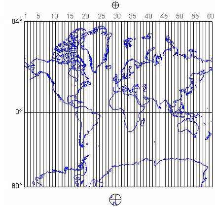
The illustration above depicts UTM zones as if they were uniformly "wide" from the Equator to their northern and southern limits. In fact, since meridians converge toward the poles on the globe, every UTM zone tapers from 666,000 meters in "width" at the Equator (where 1° of longitude is about 111 kilometers in length) to only about 70,000 meters at 84° North and about 116,000 meters at 80° South.

To clarify this, the illustration below depicts the area covered by a single UTM coordinate system grid zone. Each UTM zone spans 6° of longitude, from 84° North to 80° South. Each UTM zone is subdivided along the equator into two halves, north and south.

Figure 2.9. UTM coordinate system zone characteristics. Yellow represents areas in which UTM coordinates are valid for a given zone. Red lines parallel to the central meridian represent the two standard lines employed in each Transverse Mercator projection. These two standard lines are parallel to, and 180,000 meters east and west of, each central meridian. Each square grid cell in the illustration spans 500,000 meters on each side.

Credit: © Penn State University, is licensed under CC BY-NC-SA 4.0

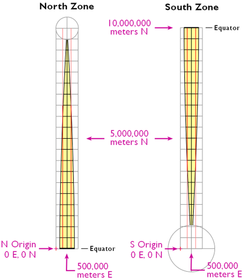
The illustration above shows how UTM coordinate grids relate to the area of coverage illustrated above. The north and south halves are shown side by side for comparison. Each half is assigned its own origin. The north south zone origins are positioned to south and west of the zone. North zone origins are positioned on the Equator, 500,000 meters west of the central meridian for that zone. Origins are positioned so that every coordinate value within every zone is a positive number. This minimizes the chance of errors in distance and area calculations. By definition, both origins are located 500,000 meters west of the central meridian of the zone (in other words, the easting of the central meridian is always 500,000 meters E). These are considered "false" origins since they are located outside the zones to which they refer. UTM eastings specifying places within the zone range from 167,000 meters to 833,000 meters at the equator. These ranges narrow toward the poles. Northings range from 0 meters to nearly 9,400,000 in North zones and from just over 1,000,000 meters to 10,000,000 meters in South zones. Note that positions at latitudes higher than 84° North and 80° South are defined in Polar Stereographic coordinate systems that supplement the UTM system.

The distorted ellipse graph below shows the amount of distortion on a UTM map. This kind of plot will be explained in more detail below; the key thing to note here is that the size and shape of features plotted in red indicate the amount of size and shape distortion across the map (a wide range in sizes indicates substantial area distortion, a range from circles to flat ellipses indicates substantial shape distortion). The ellipses centered within the highlighted UTM zone are all the same size and shape. Away from the highlighted zone, the ellipses steadily increase in size, although their shapes remain uniformly circular. This pattern indicates that scale distortion is minimal within Zone 30, and that map scale increases away from that zone. Furthermore, the ellipses reveal that the character of distortion associated with this projection is that shapes of features as they appear on a globe are preserved while their relative sizes are distorted. Map projections that preserve shape by sacrificing the fidelity of sizes are called conformal projections. The plane coordinate systems used most widely in the U.S., UTM and SPC (the State Plane Coordinates system), are both based upon conformal projections.

Figure 2.10. The result of a Transverse Mercator projection of the world centered on UTM Zone 30. Red circles reveal the scale distortion introduced during the transformation from geographic to projected plane coordinates. On the globe, all the circles would be the same size.

Credit: © Penn State University, is licensed under CC BY-NC-SA 4.0

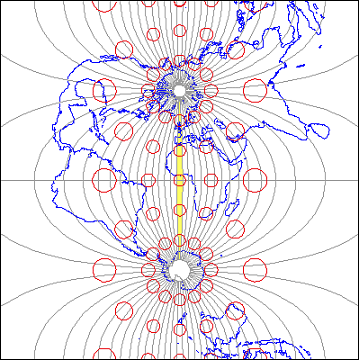
The Transverse Mercator projection illustrated above minimizes distortion within UTM zone 30 by putting that zone at the center of the projection. Fifty-nine variations on this projection are used to minimize distortion in the other 59 UTM zones. In every case, distortion is no greater than 1 part in 1,000. This means that a 1,000 meter distance measured anywhere within a UTM zone will be no worse than + or - 1 meter off.

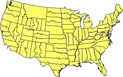
One disadvantage of the UTM system is that multiple coordinate systems must be used to account for large entities. The lower 48 United States, for instance, spreads across ten UTM zones. The fact that there are many narrow UTM zones can lead to confusion. For example, the city of Philadelphia, Pennsylvania is east of the city of Pittsburgh. If you compare the Eastings of centroids representing the two cities, however, Philadelphia's Easting (about 486,000 meters) is less than Pittsburgh's (about 586,000 meters). Why? Because although the cities are both located in the U.S. state of Pennsylvania, they are situated in two different UTM zones. As it happens, Philadelphia is closer to the origin of its Zone 18 than Pittsburgh is to the origin of its Zone 17. If you were to plot the points representing the two cities on a map, ignoring the fact that the two zones are two distinct coordinate systems, Philadelphia would appear to the west of Pittsburgh. Inexperienced GIS users make this mistake all the time. Fortunately, GIS software is getting sophisticated enough to recognize and merge different coordinate systems automatically.

2.2.4 State Plane Coordinates

The UTM system was designed to meet the need for plane coordinates to specify geographic locations globally. Focusing on just the U.S., in consultation with various state agencies, the U.S. National Geodetic Survey (NGS) devised the State Plane Coordinate System with several design objectives in mind. Chief among these were:

1. plane coordinates for ease of use in calculations of distances and areas;
2. all positive values to minimize calculation errors; and
3. a maximum error rate of 1 part in 10,000.

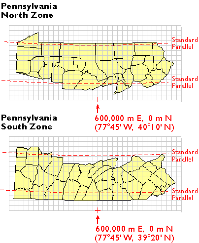
As discussed above, plane coordinates specify positions in flat grids. Map projections are needed to transform latitude and longitude coordinates to plane coordinates. The designers of the SPCS did two things to minimize the inevitable distortion associated with projecting the Earth onto a flat surface. First, they divided the U.S. into 124 relatively small zones that cover the 50 U.S. states. Second, they used slightly different map projection formulae for each zone, one that minimizes distortion along either the east-west or north-south line depending on the orientation of the zone. The curved, dashed red lines in the illustration below represent the two standard lines that pass through each zone. Standard lines indicate where a map projection has zero area or shape distortion (some projections have only one standard line).

As shown below, some states are covered with a single zone while others are divided into multiple zones. Each zone is based upon a unique map projection that minimizes distortion in that zone to 1 part in 10,000 or better. In other words, a distance measurement of 10,000 meters will be at worst one meter off (not including instrument error, human error, etc.). The error rate varies across each zone, from zero along the projection's standard lines to the maximum at points farthest from the standard lines. Errors will be much lower than the maximum at most locations within a given SPC zone. SPC zones achieve better accuracy than UTM zones because they cover smaller areas, and so are less susceptible to projection-related distortion.

Figure 2.11. The U.S. State Plane Coordinate system of 1983 consists of 124 zones. Each zone is a distinct plane coordinate system. (Alaska and Hawaii not shown).

Credit: from Scales and Transformations by David DiBiase, and licensed under CC BY-NC-SA 4.0

As we have seen above, positions in any coordinate system are specified relative to an origin. Like UTM zones, SPC zone origins are defined so as to ensure that every easting and northing in every zone are positive numbers. As shown in the illustration below, SPC origins are positioned south of the counties included in each zone. The origins coincide with the central meridian of the map projection upon which each zone is based. The false origin of the Pennsylvania North zone, is defined as 600,000 meters East, 0 meters North. Origin eastings vary from zone to zone from 200,000 to 8,000,000 meters East.

Figure 2.12. Schematic view of two State Plane Coordinate System zones, showing the counties that make up each zone (in yellow), the origins of each zone, and the standard lines of the map projections upon which the zones are based, along which scale distortion is zero.

Credit: © Penn State University, is licensed under CC BY-NC-SA 4.0

The SPCS zones are identified with a 4 digita FIPS code, the first two digits represents the state and the second the zone (e.g., PA has a FIPS code of 37 with 2 zones, 1 and 2, thus 3701 for the nothern zone and 3702 for the sourthern). The starting "0" for states in the 1-9 range is typically dropped; thus for CA, as an example, the most norther SPCS zone is 401.

One place you can look up all zone numbers is here: USA State Plane Zones NAD83

Shown below is the southwest corner of the same 1:24,000-scale topographic map used as an example above. Along with the geographic coordinates (40 45' N latitude, 77° 52' 30" W longitude) of the corner and UTM tick marks discussed above, SPCS eastings and northings are also included. The tick labeled "1 970 000 FEET" represents a SPC grid line that runs perpendicular to the equator and 1,970,000 feet east of the origin of the Pennsylvania North zone. Notice that, in this example, SPC system coordinates are specified in feet rather than meters. The SPC system switched to use of meters in 1983, but most existing topographic maps are older than that and still give the specification in feet (as in the example below). The origin lies far to the west of this map sheet. Other SPC grid lines, called "northings" (the one for 220,000 FEET is shown), run parallel to the equator and perpendicular to SPC eastings at increments of 10,000 feet. Unlike longitude lines, SPC eastings and northings are straight and do not converge upon the Earth's poles.

Figure 2.13. Southwest corner of a USGS topographic map showing grid ticks and labels for three different coordinate systems, including the SPC coordinate system.

Credit: U.S. Geological Survey, public domain.

SPCs, like all plane coordinate systems, pretend the world is flat. The basic design problem that confronted the geodesists who designed the State Plane Coordinate System was to establish coordinate system zones that were small enough to minimize distortion to an acceptable level, but large enough to be useful.

Most SPC zones are based on either a Transverse Mercator or Lambert Conic Conformal map projection whose parameters (such as standard line(s) and central meridians) are optimized for each particular zone. "Tall" zones like those in New York state, Illinois, and Idaho are based upon unique Transverse Mercator projections that minimize distortion by running two standard lines north-south on either side of the central meridian of each zone, much as the same projection is used for UTM zones. "Wide" zones like those in Pennsylvania, Kansas, and California are based on unique Lambert Conformal Conic projections (see below for more on this and other projections) that run two standard lines (standard parallels, in this case) west-east through each zone. (One of Alaska's zones is based upon an "oblique" variant of the Mercator projection. That means that instead of standard lines parallel to a central meridian, as in the transverse case, the Oblique Mercator runs two standard lines that are tilted so as to minimize distortion along the Alaskan panhandle.)

These two types of map projections share the property of conformality, which means that angles plotted in the coordinate system are equal to angles measured on the surface of the Earth. As you can imagine, conformality is a useful property for land surveyors, who make their livings measuring angles.

This section has hinted at some of the characteristics of map projections and how they are used to relate plane coordinates to the globe. Next, we delve more deeply into the topic of map projections, a topic that has fascinated many mathematicians and others over centuries.