The terms quality control and quality assurance are often used somewhat interchangeably, or in tandem, to refer to a multitude of tasks performed internally by the data producer and externally, or independently, by the data purchaser. For the purposes of this course, we will adopt the following definitions provided in Maune (2007):
Quality Assurance (QA) –
Steps taken: (1) to ensure the end client receives the quality products it pays for, consistent with the Scope of Work, and/or (2) to ensure an organization’s Quality Program works effectively. Quality Programs include quality control procedures for specific products as well as overall Quality Plans that typically mandate an organization’s communication procedures, document and data control procedures, quality audit procedures, and training programs necessary for delivery of quality products and services.
Quality Control (QC) –
Steps taken by data producers to ensure delivery of products that satisfy standards, guidelines, and specifications identified in the Scope of Work. These steps typically include production flow charts with built-in procedures to ensure quality at each step of the work flow, in-process quality reviews, and/or final quality inspections prior to delivery of products to a client.
Independent QA/QC –
Steps taken by a QA/QC specialty firm, hired by the client (e.g., government or data producer) to independently validate the effectiveness of the data producer’s quality processes.
Quantitative accuracy assessment (testing remotely sensing mapping products against ground control checkpoints) falls under the category of independent QA/QC defined above. It is normally conducted by an individual or organization that had no involvement in the data acquisition or production. The ground check points are not made available to the data producer; so that the final coordinate comparison is truly an independent test of spatial accuracy.
Before we delve further into the topic of accuracy assessment, we must define exactly what we mean when we use the term "accuracy" and distinguish it from the related term, "precision."
Absolute accuracy -
Absolute accuracy is the closeness of an estimated, measured, or computed value to a standard, accepted, or true value of a particular quantity. In mapping, a statement of absolute accuracy is made with respect to a datum, which is, in fact, also an adjustment of many measurements and has some inherent error. The statement of absolute accuracy is made with respect to this reference surface, assuming it is the true value.
Relative accuracy -
Relative accuracy is an evaluation of the amount of error in determining the location of one point or feature with respect to another. For example, the difference in elevation between two points on the earth's surface may be measured very accurately, but the stated elevations of both points with respect to the reference datum could contain a large error. In this case, the relative accuracy of the point elevations is high, but the absolute accuracy is low.
Precision -
Precision is a statistical measure of the tendency for independent, repeated measurements of a value to produce the same result. A measurement can be highly repeatable, therefore very precise, but inaccurate if the measuring instrument is not calibrated correctly. The same error would be repeated precisely in every measurement, but none of the measurements would be accurate.
Independent check points are used to assess the absolute accuracy of a remotely-sensed dataset. Realize, however, that the check point coordinates are also derived from some form of surveying measurement, and there is also some degree of error associated with them. It is customary to require that the check points be at least three times as accurate as the targeted accuracy of the mapping product being tested; for example, if an orthophoto product is specified to have no more than 1 foot of horizontal error, then the check points used to test the orthophoto product should themselves contain no more than 1/3 foot of error.
As you will learn in this lesson, quantification of error and accuracy relies on statistical principles of probability. Accuracy standards for imagery and terrain data are described in probabilistic terms; for example, one might report that the coordinates of an object derived from an orthophoto image were tested against independent ground checkpoints and were shown to agree within certain number of feet at the 90% or 95% percent confidence level. Confidence level refers to the probability that any other independently tested point in the dataset will differ from its true value by no more than the stated amount.
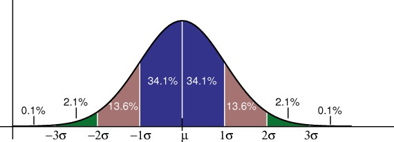
The statistical model used to determine this confidence level is most often the normal, or Gaussian, distribution. The assumption underlying the use of this statistical model is that the errors associated with repeated measurements of the same physical quantity will distribute themselves according to a particular probability density function, the Gaussian "bell curve," shown below in Figure 1. Measurements very close to the true value are the most likely, but measurements that deviate from the true value will occur on a less frequent, yet predictable, basis. The peak of the bell curve represents the mean of all measurements and the true value of the variable in question; the sloping sides of the curve represent the probability of observing values that deviate from the mean. In a normal distribution, the deviations must be distributed symmetrically about the mean; in other words, high values are as likely as low values. The width of the curve represents the range of probable values with respect to the true value, or the magnitude of probable error.
The statistical parameter used to quantify the width of the Gaussian bell curve is the standard deviation, known as sigma, also often referred in the GIS world to as the root-mean-square-error (RMSE). Given a large enough sample of measurements, 68% will fall within one sigma of the mean, 95% will fall within about two sigma (1.96*sigma, to be precise), and 99.8% will fall within three sigma. When comparing a spatial dataset to a sample of ground checkpoints, one can plot the differences between the observed coordinates and the checkpoint coordinates, compute the mean error and RMSE using standard statistical formulas, and report accuracy at the 95% confidence limit as a function of RMSE.
Remember that the basic assumption one makes when applying the normal distribution as an appropriate error model is that there are no irregularities or artifacts in the data that would cause the actual error distribution to differ from the ideal Gaussian bell curve. Furthermore, for RMSE to apply as a statement of absolute positional accuracy, there can be no biases or systematic errors in the dataset that cause the average error to be significantly non-zero. Remotely sensed datasets may contain systematic errors, either due to characteristics of the sensor or characteristics of the target. In the lesson material to come, you will see examples of this, and you will see how the statistics used in accuracy assessment help to point out these biases and diagnose their cause.