One of the first points to make in a discussion about spatial accuracy of orthorectified imagery is that accuracy is completely unrelated to spatial resolution. The size of a pixel has no physical bearing on the accuracy of its location in the ground coordinate system. Spatial accuracy depends only on the quality of the georeferencing, either as applied from ground control with aerotriangulation or provided by direct georeferencing. The difference between spatial accuracy and spatial resolution is often overlooked or unrecognized by the layman, and it is often not made clear to the uninitiated public consumer in marketing literature or by the news media.
The size of an object that can be seen in an image, compared to the accuracy of its location as derived from the image, may be significantly different. For example, the standard USGS and NAIP DOQQ products were produced at a 1-meter GSD with a targeted horizontal accuracy of about 10 meters at the 90% confidence level compared to ground surveyed checkpoints. When circumstances and budgets permit, it is desirable to specify a spatial accuracy requirement that is comparable to the size of a pixel in ground units. For example, if the output image pixel size is 1 meter, then the spatial accuracy requirement might be defined such that each 1-meter pixel in the image was assured to be within 2 meters of its "true" location in the ground coordinate system at the 95% confidence limit. The general rule of thumb is to target a root-mean-square-error (RMSE) for spatial accuracy equivalent to the size of a pixel (GSD) in the output image. In practice, and depending on the end user application, it is not always possible or necessary to follow this rule. If the primary purpose of the imagery is simply to identify objects and measure their size relative to each other, then the absolute spatial accuracy in terms of ground coordinates may be less important than relative accuracy or spatial resolution. If the objective is to create secondary map products from the orthorectified imagery, such as building footprints or road centerlines, then the absolute accuracy should be comparable to resolution.
In the interest of economy, some image data products are generated using control extracted from other image sources, rather than using new ground control or direct georeferencing data acquired along with the new imagery. This is akin to the exercise we performed in the final part of the Lesson 3 lab, using image points I provided as a source of control for orthorectification. Many USDA NAIP DOQQs use USGS DOQQs as a source of georeferencing control. Furthermore, they often use the USGS DOQQs as a source of "independent" check points; so that the accuracy that is reported is a comparison to the USGS image, not the actual ground. The following quote, consistent with USDA NAIP program specifications, is extracted from the metadata of the 2005 NAIP DOQQs for the state of Minnesota, "the source quarter-quad files are 2 meter ground sample distance (GSD) orthoimagery rectified to a horizontal accuracy of within 10 meters of reference digital orthophoto quarter quads (DOQQ's) from the National Digital Ortho Program (NDOP)." This is a statement of relative accuracy, not of absolute accuracy. One must read the metadata carefully to understand the distinction; relying on software, simply reading the RMSE from a metadata field, may lead to faulty assumptions about the spatial accuracy of the data one is using for analysis.
Data Validation
Acceptance of an orthorectified image deliverable should validate all the product specifications defined by the end user. There are three general categories of quality control and quality assurance checks and tests:
- Data Integrity - do the files contain what they are supposed to contain?
- Spatial Accuracy - do the data products meet the end user requirements for horizontal accuracy?
- Aesthetics - do the data products meet the customer's expectations in terms of color balancing, edge matching from photo to photo, and other general image quality characteristics?
Simply viewing the imagery in a GIS environment accomplishes the data integrity step. This cursory view can ensure that:
- individual image files are in the correct format and the files have not been corrupted;
- complete coverage of the area of interest has been achieved;
- accurate georeferencing information exists for each image file, in the specified coordinate system;
- size of image pixels matches the data product specification.
Quantitative Assessment
Orthorectified imagery is very often used as a visual backdrop to other GIS data or as a source for image interpretation and collection of point, line, or polygon features to be used in GIS. Because of this widespread use as a base map, quantitative accuracy assessment is one of the most important aspects of orthophoto quality assurance and acceptance testing.
An orthophoto is essentially a 2-dimensional product. As we learned in Lesson 3, the fidelity and accuracy of the terrain model used in the rectification process has an impact on the horizontal accuracy of the orthophoto; however, the image dataset has no elevation information contained explicitly within it. Horizontal accuracy is the only relevant spatial accuracy assessment metric. The end user's accuracy specification is commonly stated as a root-mean-square-error (RMSE) based on measurements of well-defined points in the imagery compared to independent survey measurements of higher accuracy serving as ground truth. The definition of a well-defined point, guidance on the selection and surveying of these checkpoints, and the methodology for calculating the RMSE is documented in the National Standard for Spatial Data Accuracy (NSSDA) published by the US Federal Geographic Data Committee.
For historical reasons, mapping accuracies are commonly specified at the 95% confidence limit. A typical accuracy statement accompanying an orthophoto deliverable would be "Tested ____ (meters, feet) horizontal accuracy at 95% confidence level," and the numerical value supplied is RMSE * 1.7308. This statement of accuracy assumes that no systematic errors or biases are present in the data and that the individual checkpoint errors follow a normal distribution, independent in the x and y directions. Note that the multiplier for the RMSE is 1.7308, rather than the 1.96 factor stated in the Introduction page of this lesson. Horizontal error is a circular error, a combination of the independent linear errors in the x and y dimensions.
Most professional practitioners involved in the design of a remote sensing data acquisition know how to design a project to meet the designated accuracy specification. When errors exceed specification, there is usually a systematic cause. Common problems are instrument misalignment or miscalibration, georeferencing system drifts, and blunders in datum or coordinate system conversion. Systematic errors such as these can be detected by examining other statistical metrics and plotting the spatial distribution of the errors. In a dataset containing systematic errors, the mean of the errors will be non-zero and the entire may be shifted north, south, east, or west from its proper location. Systematic trends are easily detectable and can usually be related to a physical cause. Once the cause has been determined, systematic errors can often be corrected by reprocessing the data. Only when systematic errors have been successfully removed does the RMSE or 95% confidence statement give the user a true indication of the absolute accuracy of the data product.
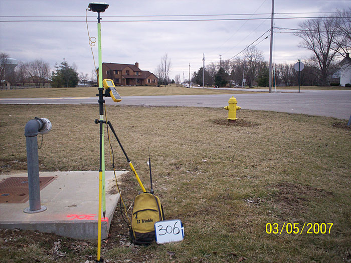
The process of accuracy assessment begins with collection of a number of ground checkpoints, usually surveyed with GPS, accompanied by a set of field sketches and photographs to aid the image analyst in proper identification in the orthophoto image. Figure 2 shows an example of such a check point, chosen because it can be clearly and unambiguously identified in the orthophoto to be tested.
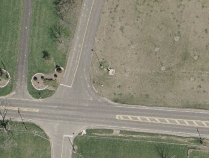
The survey sketch shown in Figure 3 above is an important complement to the digital photograph. The sketch provides additional information about the vicinity of the point that helps the image analyst navigate to the correct vicinity of the point. Armed with the surveyed coordinate derived GPS, the digital photo, and the field sketch, the image analyst should be able to locate the point within the project area, identify the correct orthophoto image within the project database to be examined, and navigate to the exact location of the point, as shown in Figure 4. The surveyed coordinates, derived from GPS, are then compared to the coordinate readout from the orthophoto in GIS or CAD software.
The image analyst visits and records the coordinates for each surveyed checkpoint in the orthophoto imagery. This can be done quite easily in GIS software. The survey results can be imported as a point file and overlaid on the orthophoto with identifying labels. The points should fall very close to the correct location, and the image analyst has only to confirm the exact location, using the photo and the sketch. The image point measurements are recorded in another point file. A table of coordinates can be exported from the GIS or CAD software and used to generate graphs and statistics, such as mean error in each direction, RMSE and 95% confidence values.
Qualitative Assessment
The final step of acceptance testing involves an examination of general image quality. The imagery for a large project may have been flown over a period of weeks under varying lighting conditions. Matching and balancing the brightness, contrast, and color tones may require use of image processing software.
The USDA developed a set of documents describing the type of visual artifacts they commonly see in orthophoto deliverables to the NAIP program. Because this type of visual inspection goes beyond the intended scope of this lesson, it won't be discussed in the lesson material. Feel free to review the referenced documents, which have been made available through the course download site. These are specific to a particular federal imagery program; however, the types of artifacts encountered and the image processing techniques recommended to overcome them can be widely applied.
- FSA User Sensitivity Study for Quality of National Agricultural Imagery Program (NAIP) Imagery - Interim Technical Report looks at end user sensitivity to aesthetic issues, such as noise, sharpness, color registration, color saturation, color balance, and tonal variation. The report is a valuable example because it examines the impact of these issues in the context of the intended application. While aesthetic defects may be distracting or annoying from a purely aesthetic point of view, the prescribed remedy may not produce sufficient benefits to justify the cost or time required to implement.
- Aerial Photography Field Office-National Agriculture Imagery Program (NAIP) Suggested Best Practices - Final Report provides guidelines and recommendations for the use of image processing techniques to effectively remedy defects identified in the User Sensitivity Study.
- Aerial Photography Field Office-Scaled Variations Artifact Book provides a number of graphic examples of the defects before and after image processing remedies have been applied.