Lessons
This is the course outline.
Welcome to GEOG 585 - Open Web Mapping
Geography 585: Open Web Mapping is a 10-week online course that gives you experience with sharing geographic information on the Internet using free and open source software (FOSS) and open specifications. It is an elective course in Penn State's online geospatial education programs, including the Master of Geographic Information Systems. The lessons are freely visible online as open courseware; however, if you would like to receive official credit for the course and complete the lessons with instructor and peer feedback, you should register for the course through the Penn State World Campus.
The two main purposes of Geog 585 are to help you understand the importance of web services and to give you some experience making web maps with FOSS and open standards. You could certainly implement web services using proprietary software, too; however, the cost of a proprietary GIS server package makes FOSS an attractive area of study for basic web mapping tasks.
The purpose of Geog 585 is not to promote FOSS over proprietary software, or vice versa (you could find plenty of materials on the Internet debating this subject); however, Geog 585 should familiarize you with the capabilities and shortfalls of the current FOSS landscape to the point that you can make an informed decision about whether to use FOSS in your own web mapping tasks.
This course requires you to do some programming with JavaScript and the Leaflet API. You don't have to know anything about Leaflet yet, but it is required that you have:
- enough formal experience with writing computer programs or scripts that you are comfortable identifying and using fundamental constructs such as variables, loops, decision structures, error handling, objects, and so forth. Geog 485 [1] satisfies this prerequisite. Exceptions require equivalent programming experience and instructor approval;
- enough experience with JavaScript that you are able to easily identify the above constructs when you see them in a piece of JavaScript code. Geog 863 [2] satisfies this prerequisite, or you can do your own preparation using the W3Schools JavaScript tutorial [3];
- enough experience with HTML and CSS that you are easily able to view and interpret the basic elements of page markup, such as the head, body, script tags, and so forth. Geog 863 [2] satisfies this prerequisite, or you can do your own preparation using the W3Schools HTML tutorial [4].
Lesson 1: FOSS and its use in web mapping
The links below provide an outline of the material for this lesson. Be sure to carefully read through the entire lesson before returning to Canvas to submit your assignments.
Note: You can print the entire lesson by clicking on the "Print" link above.
Overview
In this lesson, you'll learn some of the history of web mapping and why web services are so important. You'll also learn about free and open source software (FOSS) and the benefits and drawbacks of using it. Finally, you'll get the chance to install and use QGIS, a FOSS solution for desktop GIS work. QGIS will help you preview and manipulate your data as you prepare to create web maps later in the course.
Objectives
- Describe the roles of clients, servers, and requests and how they contribute to web service communication patterns.
- Identify benefits and challenges to FOSS and how they should be weighed when choosing a software platform.
- List common FOSS solutions for general computing and GIS and discuss how you have seen these used in the “real world.”
- Recognize when and how FOSS might be used in a “hybrid” model with elements of proprietary software.
- Add and symbolize GIS data in QGIS.
Checklist
- Read the Lesson 1 materials on this page.
- Complete the walkthrough and post your final screenshot as a post on the "Lesson 1 walkthrough result forum" on Canvas.
- Complete the Lesson 1 assignment, which involves readings and a discussion.
The history and importance of web mapping
For decades, most digital geographic information was confined for use on desktop-based personal computers (PCs) or in-house mainframes and could not be easily shared with other organizations. GIS analysts would access data from their own workplace computers that were often connected to a central file server somewhere in the office. Specialized software was required to view or manipulate the data, effectively narrowing the audience that could benefit from the data.
With mass uptake of the Internet in the mid-1990s, people began thinking about how maps and other geographic information could be shared across computers, both within the organization and with the general public. The first step was to post static images of maps on HTML pages; however, people soon realized the potential for interactive maps. The first of these, served out by newborn versions of software such as Map Server and Esri ArcIMS, were horrendously pixelated, slow, and clunky by today's standards. Limited by these tools, cartographers had not yet arrived en masse on the web mapping scene, and most of the maps looked hideous. However, these early interactive web maps were revolutionary at the time. The idea that you could use your humble web browser to request a map anywhere you wanted and see the resulting image was liberating and exciting. See Brandon Plewe's 1997 book GIS Online (findable in many university geography libraries) to get a feel for the web mapping landscape at this time period.
These early, dynamically drawn web maps ran into challenges with speed and scalability (the ability to handle many simultaneous users). The server could only accommodate a limited number of map requests at a time before slowing down (at best) and crashing (at worst). Web maps matured significantly in these two metrics when websites began to serve out tiled map images from pregenerated caches. Why ask the server to draw every single map dynamically when you could just put forward an initial investment to predraw all possible map extents at a reasonable set of scales? Once you had the map images drawn and cached, you could serve out the images as a tiled mosaic. Each tiled map request was satisfied exponentially faster than it would take to serve the map dynamically, allowing for a server to accommodate hundreds of simultaneous users.
Following the lead of Google Maps, many sites began serving out “pre-cooked” tiled map images using a creative technique known as Asynchronous JavaScript and XML (AJAX) that eliminated the ubiquitous and annoying blink that occurred after any navigation action in earlier web maps. Now you could pan the map forever without your server gasping for breath as it tried to catch up.
Cartographers, who had largely been resigned to trading aesthetics for speed in web maps, also realized the potential of the tiling techniques. No longer would the number of layers in a map slow down the server: once you had pregenerated the tiles, you could serve a beautiful map just as fast as an ugly one. Web maps became an opportunity to exercise cartographic techniques and make the most attractive map possible. Thus were born the beautiful, fast, and detailed “web 2.0” basemaps that are common today on Google, Microsoft Bing, OpenStreetMap, and other popular websites.
As web browsers increased in their ability to draw graphics using technologies such as SVG and later WebGL, the possibilities for interactivity arose. On-the-fly feature highlighting and HTML-enriched popup windows became common elements. For several years, developers experimented with plug-ins such as Adobe Flash and Microsoft Silverlight for smooth animation of map navigation and associated widgets. More recently, developers are abandoning these platforms in favor of new HTML5 standards recognized by the latest web browsers without the need for plug-ins.
Although maps had arrived on the browser by the mid-2000s, they were still largely accessed through desktop PCs. The widespread adoption of smartphones and tablets in subsequent years only increased the demand for web maps. Mobile devices could not natively hold large collections of GIS data, nor could they install advanced GIS software; they relied on web or cellular connections to get maps on demand. These connections were either initiated by browsers on the device, such as Safari, or native applications installed on the device and built for simple, focused purposes. In both cases, GIS data and maps needed to be pulled from the organization's traditional data silos and made available on the web.
The importance of web services
All the above web mapping scenarios are possible because of web services. If you search the Internet, you'll find many definitions of web services and can easily get yourself confused. For the purposes of this course, just think of a web service as a focused task that a specialized computer (the server) knows how to do and allows other computers to invoke. You work with the web service like this:
- You invoke the web service by making a request from an application (the client). To make this request, you usually use HTTP, a standard protocol that web browsers use for communicating between clients and servers. The request contains structured pieces of information called parameters. These give specific instructions about how the task should be executed.
- The server reads the request and runs its web service code, considering all the parameters while doing so. This produces a response, which is usually a string of information or an image.
- The server sends you the response, and your application uses it.
Examine how the following simple diagram describes this process, returning a map of current precipitation:
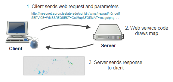
Now, for an example. Let's suppose that you've identified the URL of a web service out there somewhere that draws maps. You make a request by constructing a URL (http://...) containing the address of the web service and various parameters for the map, such as the format of the image you want to receive (JPG, PNG, etc.), bounding box (coordinates defining the geographic area you want to see mapped), and map scale. You paste this into your browser's address bar and the server sends you a response containing the map image you requested.
Here's an example of just such a request, using a radar map of the United States. First, see if you can identify some of the parameters in the URL. Then take a guess at what the response will look like when you get it back. Then click the link to invoke the web service and get the response:
As you examined the URL of this request, you might have noticed parameters indicating the width and height of the image, the image format, the image background transparency, and the bounding coordinates of the map to be drawn. These parameters provide specific details about how the web service should run its map drawing code. You see these parameters reflected in the response image sent back to your browser when you clicked the link. In a future lesson, you'll learn about more of the parameters in the request above.
Not all web requests invoke web service code. Some web requests just return you a file. This is how tiled maps work, and this is why they are so fast. You'll learn more about tiled maps in a later lesson, but examine the following request for a specific zoom level, row, and column of a tile:
http://a.tile.openstreetmap.org/15/11068/19742.png [7]
The request drills down into the server's folder structure and returns you the requested PNG image as a response. No special code ran on the server other than the basic file retrieval, therefore you could argue that a web service was not invoked. However, this type of simple web request is also an important part of many web maps.
At this point, you might be thinking, “I've used web maps for years and I have never had to cobble together long clunky URLs like this. Have I been using web services and other web requests?” Absolutely, yes. As you navigate Google Maps, your company's online map site, and so on, your browser is sending hundreds of web requests similar to this one. You've just never needed to know the details until now. When you begin setting up your own GIS server or designing your own client web application, it becomes important to understand the theory and architecture behind web traffic.
Not all web services use the same format of URL and parameters. In this course, you'll learn about some of the most common formats for online web services, especially ones that have been openly developed and documented to work across software packages.
Viewing web service requests in real time
Here's a simple way you can view web requests made “behind the scenes” by your browser as you navigate a website. These instructions are for the tools provided by Mozilla Firefox. Chrome and other browsers have similar tools that typically go under the name "developer tools" or "web tools" and should not be difficult to locate.
- Open Mozilla Firefox (if it's not already running) and from the main menu choose More Tools -> Web Developer Tools. This will open the developer tools window in the bottom part of your browser. At the top of the window, you can see different tabs "Inspector", "Console", and so on. Select the one called "Network", which is for monitoring network traffic. In addition to the "Network", the "Console" tab will be important for this course because it will show the Javascript and other error messages if something is not right with your Javascript code.
- Make sure that All is highlighted in the menu of filters below the tabs (which will contain items such as All, HTML, CSS, JavaScript, etc.).
- Hit this website for the Portland TriMet interactive system map [8] (note that this site exclusively uses FOSS mapping software).
- Navigate the map of the Portland transportation system.
- Notice the web requests as they are sent. You'll see a lot of requests appearing for map tiles.
- Hover over a request to see its full URL. If the response is an image, hovering over the little thumbnail in front of the URL will show a larger version of the returned image.
- When an entry in the list of requests is selected, the right part of the window will show many additional technical info about the request and response.
This kind of developer tool will be valuable to you later in the course as you develop your own web maps, mainly for troubleshooting scenarios where you expect a map to show up and your browser does not send you the expected response.
References
Plewe, B. (1997). GIS online: Information retrieval, mapping, and the Internet. OnWord Press.
Understanding FOSS and its use in web mapping
The term “free and open source software” (hereafter referred to as FOSS) includes a number of ideas that can invoke complex and even emotional discussions within the technical community. To begin to describe this term, it's important to understand that software development is more enigmatic and artistic than other crafts in the tech industry [9], such as computer chip design. Software cannot be seen, touched, tasted, or described in a physical sense, other than the number of megabytes it occupies on your computer. Software often begins as ideas on a whiteboard, which are then encapsulated into intangible “classes” and "objects" of code by a programmer. These are then assembled into invokable sets of concrete tasks and dressed with a user interface of buttons, menus, and icons that require a whole other skillset of aesthetic design.
As a result of all this work, software is an empowering technology that enables a person to make practical use of computer hardware. In fact, specialized software can often cost much more than the physical machine that it runs on. Software is your window into printing, painting, calculating, storing data, and, in our case, making maps.
Given the value of software, it's no surprise that commercial businesses invest millions in researching, developing, and selling proprietary software. They protect it through patent and copyright laws. They obfuscate (scramble) the code to make it harder to copy or reverse engineer. Commercial software development has become a successful enterprise whose resulting tools have shaped our work and home environments.
At the same time, some software users and developers have advocated that there are benefits from making software source code freely visible and able to be modified or shared without legal or technical restraint. Business benefits, technical benefits, and moral arguments have been invoked in support of this concept of “free and open source software.”
It's possible to get confused when learning about FOSS, because the word “free” carries several meanings in the English language. A common analogy describing the F in FOSS is “free as in free speech, not free beer.” In other words, FOSS is “free” in the sense that it is open and amenable to use and modification. (You may sometimes see the term Free/Libre [10] Open Source Software (FLOSS) used to communicate this idea.) A whole range of license types [11] are used with FOSS that specify the conditions surrounding the modification and reuse of the software, along with the attribution required on any derived products.
While the selling of FOSS is not necessarily restricted, FOSS is usually available free of charge. All of the software we'll use in this course can be downloaded directly from the Internet and requires no fee, although donating a few dollars to your favorite project is a good way to invest in its continued development.
If FOSS is usually available without cost, why is it such a successful concept? And how do people make a living from coding with it? First, it's important to mention that many developers contribute to FOSS solely for personal enjoyment and for the desire to donate their skills to a project offering wide societal benefits. They enjoy working on virtual teams and facing the challenges of rigorous software development that their ordinary “day jobs” might not offer.
At the same time, though, many individuals make a generous living by selling services and training related to FOSS, and some of these efforts may increase the quality and number of FOSS features available. For example, suppose your company invests in a FOSS package that does everything you want at $30,000 cheaper than the proprietary software alternative; however, it's missing “Feature X” that is critical for your workflows, and you don't have a programmer who can implement Feature X. Because the code for the software is all open to examination, modification, and extension, you can contract with Rock Star Programmer to implement Feature X for you for $10,000. If Feature X is widely applicable to the good of the product, and you and the contractor are okay with the idea, Feature X may eventually be rolled into the core source code so everyone can benefit from it.
Other people may not contribute frequently to FOSS projects, but can still make a profit selling support services for FOSS software. When you buy proprietary software, you often are given access to a technical support package that allows you to call and talk to an analyst if needed. Because FOSS does not offer these official support systems, enterprising individuals have stepped in to fill this void.
Finally, several new firms are building subscription-based online services that are created using open source building blocks and may even be released under open source licenses. The services are offered for a subscription cost that is lower than most organizations could achieve if they attempted to build their own comparable infrastructure or quality control procedures. Through these FOSS-based Software-as-a-Service (SaaS) offerings, the value of the free software is passed on to many buyers.
Although there are many FOSS purists out there, the decision to use FOSS does not have to result in a full migration away from proprietary software. Many businesses and governments use what might be termed a "hybrid approach," incorporating a mix of FOSS and proprietary software depending on their budget, staff skills, and technical needs.
Let's consider some of the benefits, challenges, and other considerations that the adoption of FOSS brings into your workflows.
Benefits of FOSS
As you begin the endeavor of learning to use FOSS, it's helpful to understand some of the benefits that you may see:
- Lower cost software – The reason FOSS can be offered free of charge is discussed above. Even if you have to spend a substantial amount on training, support, and consulting, these expenses may not reach the amount that you would have spent for a proprietary software package.
- More flexibility with the software – If you commit to a proprietary software vendor and you really need Feature X or Bug Fix Y, your ability to persuade the vendor to add this feature may depend on the size of your contract, how many other people want the feature, and when the next software release is available (unless you are an important enough customer to warrant a specially-built hotfix or patch). If you are a small customer and the feature you want is obscure (albeit mission critical to you), then you may wait for years and never see it added. With FOSS, you can add the feature or fix a bug at any time, and your only limits are the programmer skills you can find.
- Interoperability of the software – Many FOSS offerings attempt to abide by open specifications for data and web services so that they can interact seamlessly with other products. You will learn about some of these specifications for geospatial data later in this lesson and course.
Many proprietary software vendors indeed support the reading of open specifications, but often they will write data into proprietary data formats that can only be processed by the vendor's software. This becomes a problem when open government initiatives come into play, as demonstrated in March 2013 when the Ohio Supreme Court ruled [13](*) that Scioto County was justified in asking a citizen for a $2000 fee in response to a Public Records Act request for its GIS data. The reason for the fee: the data was inextricably intertwined with proprietary GIS software and would require extra effort to extract.
* If the link does not work for you, the reason most likely is that you are located outside the US; just search for the event on the web and you should be able to find some articles about it. - Security – Militaries, banks, and other government agencies have gravitated toward FOSS because they have a full view of its cybersecurity mechanisms and can patch or modify these according to their own desires. Some agencies will not use a new version of any software until it has passed a rigorous security certification process. FOSS allows for more agile response to issues that are brought to light during this testing.
- Ethics – Some people view the use of open source software as an ethical question. Creating and using software that is part of an intellectual commons is a powerful motivating factor for many open source advocates. The development and use of FOSS contributes to the expansion of collective human knowledge.
Challenges of FOSS
A danger of evaluating FOSS systems is to allow the potential exciting benefits to obscure the real challenges that can accompany a FOSS deployment. Some or all of the challenges below can be mitigated, but proprietary software may offer a smoother road in these areas, if you can bear the cost.
- Usability – Designing a user-friendly software product requires a much different skill set than that required to write back end software code. When the author of this course worked at a proprietary software vendor, he held the title of “Product Engineer.” These were people whom the company hired to work with the developers to design, test, and document the product. They did not write source code; they just concentrated on making a usable product.
Good product engineers are hard to find and hire, even when you are a proprietary software company with attractive salaries to offer. When the number of coders working on the back end logic of a FOSS project outweighs the effort going into user interface design, then usability can suffer. Compounding this problem is the need for frequent iteration and clear communication between software designers and developers. In the halls of a proprietary software company, this may occur more readily than in the online collaborative forums driving FOSS.
Some people who work on FOSS may vigorously debate this point, so as you work with FOSS in this course, be aware of its level of user-friendliness compared to proprietary software, and draw your own conclusions.
- Documentation availability – Just as proprietary software companies pay designers and test engineers, they also are expected to deliver a fully documented product. Thus, they hire technical writers who can produce software manuals, online tutorials, and other training. There is a business incentive for this: if your product isn't well documented, it will get a negative reputation in the community, and people will stop buying it.
When software is delivered free of charge, you rely on the benevolence of project contributors to provide any sort of documentation, much of which may be produced in the forms of wikis, tutorials, and forum posts. This can be maddeningly unstructured to someone accustomed to proprietary software whose documentation is expected to "just be there” in a single unified and searchable help system.
Some FOSS documentation is excellent, and it's important to respect the people who contribute, proofread, and translate it. However, beware that FOSS is often created by very bright individuals who can Just Figure Things Out using minimalist or fragmented sources of information, and they may expect that you can play at this same level as you try to use their product. In both proprietary software and FOSS, documentation quality can sometimes be slighted or given lower priority when the initial coding and testing have been completed and everyone is itching to get the product out the door.
Just as you did with usability, pay attention to documentation quality, and make your own judgment as you work through the course. Would you be able to figure things out without the course walkthroughs guiding you? How does it compare to the proprietary software help that you have used in the past?
- Support availability – As mentioned above, many third-party contractors offer technical support and consulting for FOSS products; however, the advantage of purchasing support from a proprietary software vendor is that the people who developed the software are often accessible by the support team. Thus, the support team can get a closer understanding of the intent, logic, design, and planned trajectory of the software. They may also maintain a large database of both internally and externally documented bugs that can help find you a workaround in a hurry. Although it may be possible for a FOSS support consultant to learn some of these same types of things, the support experience is not as smoothly integrated.
Contested points
Some aspects of FOSS and proprietary software are not as clear when it comes to deciding which type of software owns the advantage.
- Breadth of features – It can be argued (and you will see this in the Ramsey video required later in this lesson) that FOSS offers a more focused, prioritized list of features and may not be able to compete with proprietary software when it comes to sheer number and depth of features. At the same time, the flexibility of FOSS allows for infinite features to be added via plug-ins and direct modifications for the source code, something that cannot always be said for proprietary software where limited lists of new features are released via periodic updates. It should be noted here that if the proprietary software offers good APIs (in other words, programming frameworks), it, too, may be extended to a limited degree by third-party developers.
-
Quality and technical superiority – The “bugginess” of FOSS compared to proprietary software probably depends on the products in question, how mature they are, and who's developing them. FOSS advocate Eric Raymond argued that “given enough eyeballs, all bugs are shallow,” contending that it would be difficult for any major issues with FOSS to go unfixed for long among a broad community of developers. It's less clear who fixes the obscure bugs that you hit and others don't. If you can't convince someone in the FOSS community to fix it, you could at least attempt it yourself or hire a consultant.
Proprietary software vendors obviously have business incentives to fix bugs; however, they also have business incentives to NOT fix certain obscure bugs if the time, effort, and risk to do so would not provide a good return on investment. If you're a small-potatoes customer with an obscure bug holding up your project, you'd better start looking for a workaround. - Innovation – Does innovation occur more readily in a proprietary software company where large amounts of research and development dollars can be invested in full-time employees who collaborate face-to-face, or does it thrive in an environment where all the code is available for perusal and experimentation by anybody? Part of the answer may depend on how much the proprietary software company operates on a “reactive” basis as compared to a forward-looking vision. It also depends on whether the company's goals encourage certain types of development at the expense of others.
Innovation rarely occurs in a vacuum. Some would argue that innovation happens more freely when there are more elements in the intellectual commons that can be drawn upon.
Examples of widely-used FOSS
FOSS has been developed to support all tiers of system architecture. You've probably heard of (or used) some of this software before. For example, the term “LAMP stack” refers to a system that is running:
- Linux operating system
- Apache web server
- MySQL (or MariaDB) relational database
- PHP application scripting language
Other variations of this acronym exist. For example, PostgreSQL is another open source relational database that is commonly used with GIS because of the popular PostGIS extension. This results in a LAPP stack rather than a LAMP stack.
Other general-use FOSS includes the LibreOffice suite (similar to Microsoft Office), the Mozilla Firefox web browser, the Thunderbird e-mail client, the Python scripting language, and more.
FOSS use in government
Some governments have begun mandating or encouraging the use of FOSS for government offices and projects. This is especially popular in Latin America and Europe, with one of the more recent government decrees occurring in the United Kingdom [14]. Often the FOSS is implemented first on servers and back-end infrastructure, then rolled out to desktop workstations in later phases.
These policies favoring FOSS come about for different reasons. Obviously, the savings in software licenses and the flexible security models offered by FOSS are desirable, but sometimes there are political motivations to reject proprietary software companies and their countries of origin (particularly in places where the United States is perceived as imperialist). If you are interested in more reading on this topic, I recommend Aaron Shaw's study of the FOSS movement in the Brazilian government [15] and its tie to leftist politics [here is an alternative link [16] to the paper in case the other link isn't working].
FOSS and web mapping
FOSS has a strong and growing presence in the GIS industry. Some tools and utilities for processing geospatial data have been around for decades. For example, GRASS GIS [17] developed by the US Army Corps of Engineers recently turned 30 years old. To see what it looked like back then, see this old GRASS promotional video [18] narrated by none other than William Shatner. I still use this video in introductory classes to teach the benefits of GIS and the main components of a GIS system.
In this course, we'll use some of these desktop workstation GIS tools for previewing and manipulating our datasets before putting them on the web. For example, later in this lesson, you'll install and explore QGIS [19] (previously known as Quantum GIS), one of the most popular and user-friendly FOSS GIS programs.
There are also various FOSS options for exposing your GIS data on the web, either within your own office network or on the entire Internet. These include Map Server [20], QGIS Server [21], and GeoServer [22], the latter of which you will learn in this course. These software offerings take your GIS datasets and make them available as web services that speak in a variety of formats. They include a web server or are designed to integrate with an existing web server, so that your web services can reach computers outside your own office or network.
FOSS can also be used to generate sets of tiled images or vector data that you can use as layers in your web maps. In this course, you'll learn how to do this using a new tool recently integrated into QGIS.
Underlying both desktop and server GIS are the databases containing your GIS data. If you need something a little more complex than a folder of shapefiles or want to make use of spatial database types, then you can use a FOSS GIS database. These include PostGIS [23] (which is an extension to the PostgreSQL relational database) and SpatiaLite [24] (which uses the SQLite database). A lighter fare option for smaller datasets is to use standalone files of GeoJSON, KML, GeoRSS, or other well-documented text-based data formats.
To pull all your map layers together and display them on a web page, you'll use a programming framework, or API. Some of the most mature web mapping APIs are OpenLayers [25] and Leaflet [26], which you will use later in this course with the JavaScript programming language. Other popular FOSS web mapping APIs include ModestMaps [27], D3 [28], and Polymaps [29].
The role of open specifications and open data
Not to be confused with open software, open specifications are documented and mutually agreed-upon patterns of how software and digital data should behave in order to be interoperable between systems. For example, HTTP (hypertext transfer protocol) is based on a specification defining how web servers and web browsers should communicate in order to exchange information. Without open specifications, you would not be reading this web page.
How are open specifications used in web mapping?
In this course, we'll learn about two types of open specifications:
- Open data formats – Most GIS data formats are open in the sense that the way they are constructed is fully documented, and various GIS programs can read and write them. Also, the inventors of these formats have not asserted the right to any royalties when you use them.
KML and GeoJSON are some examples of GIS data formats that you can create just by writing a text document in a particular way. Most raster formats such as JPEG or PNG are also open. The shapefile is one of the most common formats for exchanging vector GIS data, because Esri has openly documented how to create a shapefile and relinquished any legal restrictions on creating shapefiles. In contrast, an example of a closed data format is the Esri file geodatabase, because Esri has not openly documented how to create a file geodatabase without using Esri tools. - Open specifications for web map services – There have been several efforts to openly document patterns that GIS web services should use when communicating with clients. The Open Geospatial Consortium (OGC) has created several of these specifications, the most popular of which is the Web Map Service (WMS). The USA weather radar service you accessed earlier in this lesson was an example of a WMS. You will learn more about the various OGC specifications later in this course.
In a document called the GeoServices REST Specification, Esri has also openly documented the form of communication used by geospatial web services in its products such as ArcGIS Enterprise and ArcGIS Online. This means that non-Esri developers are free to build applications that read or serve web services according to this pattern. Although the GeoServices REST Specification was not adopted by the OGC (a long story covered in a later lesson), it is an example of a specification that has been voluntarily made open by a proprietary software vendor.
The role of open data
In this course, we'll also be using open data, which is data that has been made available to the public free of charge and bereft of most copyright restrictions. These data may be shared by government entities, researchers, not-for-profit organizations, or ordinary citizens contributing to online projects. For example, Data.gov [30] is a popular website offering datasets collected by the US government. And, later in this course, we'll learn about one significant source of open GIS data called OpenStreetMap [31]. This is an online map consisting of voluntary contributions in the style of Wikipedia.
Open datasets are often rich and exciting to include in web maps, but there are some precautionary measures you should follow in order to be successful with using them. First, be aware that even though the data is free, you are often still required to provide attribution describing where you obtained the data. You may also be restricted from redistributing the data in any way that requires a fee. When you use an open dataset, you are responsible to carefully research and adhere to any attribution requirements. You should also make an effort to verify the data quality by examining any accompanying metadata, researching the sources and collection methods of the data, and scrutinizing the data itself.
The scope of this course
In this course, you will be getting some experience installing and using FOSS and creating web maps with it. While doing this, you will use open specifications for GIS data and web services. You'll also learn how to use open data and contribute to OpenStreetMap.
Each week, you'll complete a walkthrough explaining some FOSS tool. Following the walkthrough, I will often ask you to apply what you've learned to some of your own datasets you've found or collected. This will allow you to build up a comprehensive project as the course progresses. The goal is to produce something you can host on your personal webspace and reference in a professional portfolio.
The functionality of our web maps will be relatively simple, limited to layer display and point-and-click queries. However, the frameworks that we'll use are broadly extensible depending on how much programming you're willing and able to do.
Along the way, you'll pick up some skills with manipulating data (projecting, clipping, and so forth) with FOSS, which will hopefully prove handy throughout your GIS career. Many of these tools can be scripted with Python and other languages that you may have learned already in other GIS coursework.
Walkthrough: Installing and exploring QGIS
The first FOSS product you'll use is a GUI-based program designed for desktop workstations. It's called QGIS (kyoo-jis), although you should know that sometimes in the past it was referred to as Quantum GIS. QGIS is somewhat similar in appearance and function to Esri's ArcMap, which you've likely used in previous courses.
In this tutorial, you'll install QGIS and make a basic vector map with it. You'll use some shapefiles of downtown Ottawa, Ontario, Canada that I originally downloaded from the OpenStreetMap database.
Download the Lesson 1 walkthrough data [32] (It is a folder of shapefiles that you should extract into a folder such as c:\data).
- Visit the QGIS home page at www.qgis.org [33]. Take a few minutes to explore this introductory page and any links that look interesting. This tells you a bit about who makes QGIS and what it can do.
- From the main QGIS page, click the Download Now Button.
The usability of this page has greatly improved in the past few years. Because FOSS can run on a variety of platforms and can be built directly from source code (as opposed to running an installer program), it's not uncommon with FOSS to see mind-boggling installation instructions with all manner of parenthetical warnings, stipulations, dependencies, and links to obscure download pages. This was previously the case with QGIS, but now the experience is much smoother. - You can now choose between the latest release of QGIS or the most recent long term release (LTR) version. The advantage of using the LTR version, (version 3.28 at the point of this writing) is that the examples in this course have been tested with this version and things on your screen will look very close to what is shown in the images you will see here. If you instead want to see all the features that QGIS has to offer right now and don't mind that things may look slightly different, feel free to go ahead and install the latest release. You can also install both version and switch between them.
To start the download, click on the large green button saying "Download QGIS ..." to download the most current release, or click the small link below it "Looking for the most stable version? ..." for the LTR version. Once you've downloaded it, run through the installation wizard and accept the default options:
QGIS can also run on Mac or Linux. You will see installation instructions for these platforms, and you are welcome to use them; however, only Windows instructions are given in these lesson materials. (I know this is paradoxical for a FOSS course, but teaching you to use Linux is outside the scope of these lessons.) If you get hung up, you may be expected to troubleshoot on your own or default to a Windows machine in order to complete the exercises. If all you know is Windows, I suggest you stick with Windows for this course.
The QGIS installation will place some other shortcuts and programs on your machine, such as GRASS GIS and OSGeo4W. This is fine. In fact, we will use some of these in later lessons. - Start QGIS. You can do this through the Windows Start Menu > All Programs > QGIS (Version name/number) > QGIS Desktop (Version number).
You will notice many toolbars available. In QGIS, the button you click to add data depends on the type of data source. For example, you click different buttons to add vector files, raster files, CSV files, web service layers, and layers from databases. - Drag the toolbars and windows around and clean up your display so that the layout looks something like the screenshot below (Figure 1.3). Don't worry about the order of the toolbars; just get them off the left-hand side if they show up there. You may have to explicitly add the "Manage Layers" toolbar to perfom the next step, as described below. Adding toolbars works the same as it does with ArcMap: just right-click any empty gray area around the toolbars and select the desired toolbar from the menu that appears. Alternatively, go View -> Toolbars in the main menu bar to toggle individual toolbars on and off.
- Click the button for adding vector data:

Once you've clicked the button to add vector data, click the ... button and browse to the roads.shp file from the lesson data folder. Even though a shapefile consists of multiple files, you just need to browse to the .shp when adding a shapefile in QGIS. Now click Add and then Close to close the window again.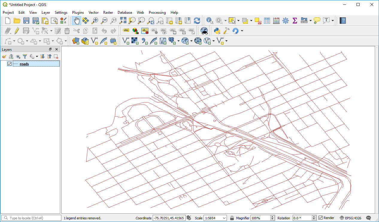 Figure 1.3
 - In the layer list, double-click the roads layer. You'll see a Symbology menu and a bunch of styling options where you can set the line color, the line width, a scale range for visibility, and labeling. Set the roads as a thin gray line.
Notice that in QGIS, you typically get a lot more symbol options if you highlight the deepest level of the symbol hierarchy, in this case, Simple line.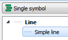
Note: During this walkthrough, I will provide general guidance about which settings to apply, and I will lead you to the correct neighborhood of dialog boxes to accomplish it; however, I will not provide point-and-click instructions for all actions. Although you may curse my name for this, I am doing it deliberately so that A) you can think about what you are doing and B) you can develop the habit of exploring new and unfamiliar software in a fearless manner. This is an essential skill if you are going to use FOSS.
That being said, it is not my intent to leave you frustrated and helpless. If something is not clear, please use the discussion forums to help each other out. I will regularly monitor the forums to make sure your question doesn't languish unanswered.
Next, we'll put some labels on the roads. - In the Layer Properties dialog box, use the Labels tab to label the roads layer with the roads' name attribute using a small gray font (this in the Text submenu). Set the label distance as 0.5 mm (this is in the Placement submenu of the Labels tab) so that the layer is not too close or too far away from the line. When working with streets, you might also want to check Merge connected lines to avoid duplicate labels (this is in the Rendering submenu). Finally, set Scale-based visibility (or Scale dependent visibility) preventing the labels from displaying when the map is zoomed out beyond 1:10000. When you are finished, you should have something like this.
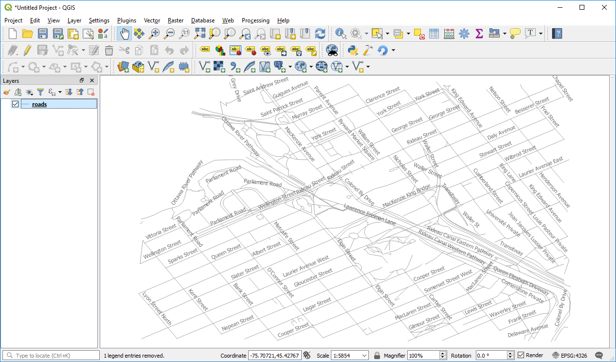 Figure 1.4
 - Add the dataset natural.shp and symbolize it as a light green fill with no outline. You will need to set the Stroke style to No pen in order to accomplish this.
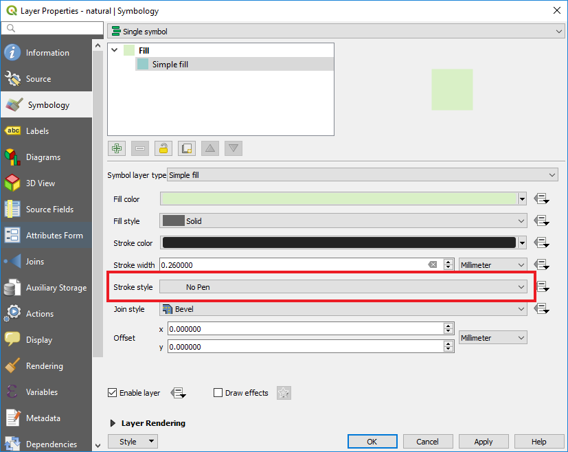 Figure 1.5
 - This is a good time to save your map. Click Project > Save As and save your map as Ottawa.qgz. It will be easiest if you save it in the same folder where your shapefiles live.
Note: You may be accustomed to using the .mxd format, and now is an opportune time to learn that .mxd is a proprietary format that is used by Esri software. QGIS uses an easily-readable XML format for storing projects (.qgs file) and the .qgz file is a zipped version of the .qgs file. You can also choose to store your project as an unzipped .qgs file and then open it in a text editor to inspect the XML code. However, .qgz is now the default file format for QGIS. - Add buildings.shp to the map, and experiment with a multilayer symbol to make the buildings “pop out.” Here's how I set this up:
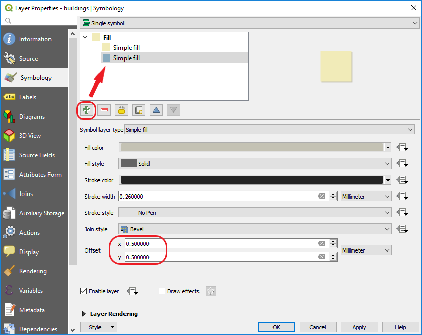 Figure 1.6
 - Add bus_stops.shp to the map, and symbolize it with an SVG marker that looks like a bus. In the Symbol layer type dropdown, select SVG marker like in the image below.
SVG stands for “scalable vector graphics.” It's a way of making marker symbols that don't get more pixelated as you expand their size. If you want a different color of marker, you can open the SVG in a graphics editing program such as the open source Inkscape, recolor and save a new version of the graphic, and then browse to it in QGIS.
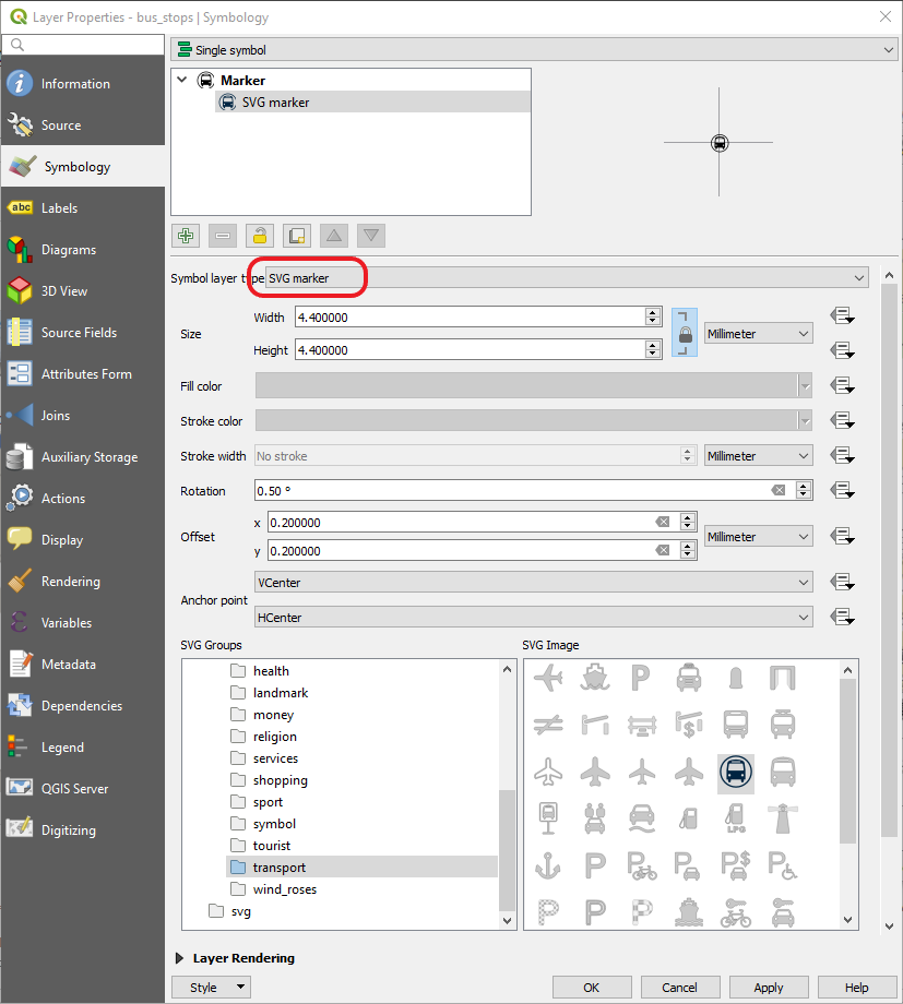 Figure 1.7
 - Set a scale range on the bus_stops layer so that it doesn't appear when zoomed out beyond 1:10000. You can do this in the Rendering tab.
This is also a good time to set a user-friendly display name for this and other layers. The display name appears in the layer list. You can change the display name in the Source tab.
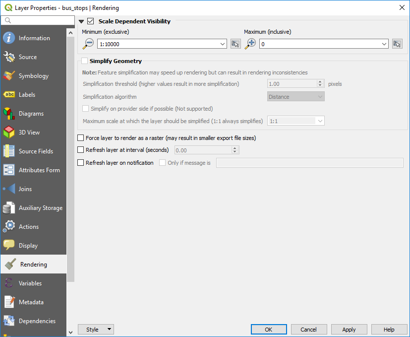 Figure 1.8
 - In the layer list, highlight the bus stops layer and click the Show Map Tips button. This button varies in appearance depending on the version of QGIS you're using, but in all cases it contains a little yellow speech bubble, like this
 . Map tips add some interactivity to the layer, a la Google Maps, so that when you hover over a stop for a short moment, the name of the corresponding bus line will be displayed. As we work with web maps during this course, we'll work with getting the same kind of interactivity for particular layers of interest.
In some versions of QGIS, this will show the bus stop ID number by default rather than the name. To remedy this, open the bus stops' Layer Properties again, go to the Display tab, and select the name field in the Display expression or Display name dropdown list.
Your map should now look something like the following: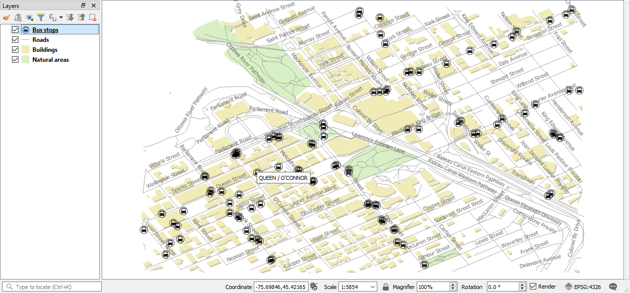 Figure 1.9
 - Save your map, then add some more shapefiles and experiment with symbolizing and labeling things in an aesthetically pleasing way.
- Post a screenshot of your beautiful QGIS map on the "Lesson 1 walkthrough result forum" on Canvas. Include some commentary about any features you found useful.
Lesson 1 assignment: Responding to FOSS
In this week's assignment, you'll watch and read several opinions on the use of FOSS within the GIS community. I will then ask you to respond to these in a detailed discussion below.
Readings
- Read the online chapter Web GIS [34] from the GIS&T Body of Knowledge, a web-based resource used by educators to outline the essential information that people should know about geographic information science and technology. This assigned chapter contains an overview of the most important things to know about Web GIS, and mentions many of the topics that will be covered throughout this course. Becoming familiar with the terms and acronyms in the glossary at the beginning will help you when you encounter these later on.
- Watch the video below: A GIS Manager's Guide to Open Source. This is a talk given by Paul Ramsey, a major contributor to PostGIS. He submits an argument for the use of FOSS and summarizes some of the FOSS tools available to geospatial professionals. Plan for 45 minutes to watch the entire video.
Click here for transcript of A Managers Guide to Open Source.
The Unknowns: A Managers Guide to Open Source
PAUL RAMSEY: I'd like to start this-- start this morning with a digression, actually, off to the side. One of my favorite pieces of poetry was composed not by a Beat poet in Greenwich Village or by a 19th century romantic, but by one Donald Rumsfeld, then Secretary of Defense, from the Pentagon press briefing room on February 12, 2002. Hart Seely later formed the secretary's words into a poem, which was published in Harper's Magazine in June 2003 as "The Unknown."
"As we know, there are known knowns. There are things we know we know. We also know there are known unknowns. That is to say, we know there are some things we do not know. But there are also unknown unknowns, the ones we don't know we don't know."
I found the same sentiments expressed less elegantly, but more forcefully, in diagram form, showing the things we know, the stuff we don't know, and the vast expanse of stuff that we don't know we don't know. And it's scary that the largest category by far is the one that we definitionally cannot comprehend, the stuff we don't know we don't know. Of course, this is an epistemological diagram of all knowledge. So, we can constrain it a bit by noting that, for practical purposes, we're really only concerned with the stuff we should know. But unfortunately, the stuff we should know still falls in all three categories.
And as IT managers, there is, amongst the stuff we should know, the stuff we should know about open source software. And I hope, at this point, we can all agree that open source is worth knowing about. The largest, most heavily trafficked companies on the internet have built their infrastructure on open source for practical, hardheaded business reasons. And open source is no longer just a technology fast follower. Leading-edge work in fields like software development tools, document search, big data analysis, and NoSQL storage, it's being spearheaded by open source projects.
And that's not because open source is just some kind of fad or just something the cool kids currently consider trendy. It's because open source is a bona fide trend. It's a trend that's been building for over 30 years. And it's changing not only the way we build software, but how we collaborate in building knowledge in general.
So I bring two perspectives to this topic, the perspective of a developer of open source software-- a hacker, a programmer, in particular on the PostGIS spatial database, which I've been involved in for 10 years-- but I also bring the perspective of a manager. I ran a small consulting company, Refractions Research, for 10 years. My goal today is to modify your internal epistemological diagrams a little bit, maybe to something more like this, and not because I expect you to all rush back home and implement open source, but because when you know more about open source, it becomes an option.
So to understand why open source is an option, it helps to have some background. So let's start with a little history. Once upon a time-- once upon a time, there was a young man with wild ideas about freedom who took on the established order of things, appeared to lose, but, in the end, changed the world forever, though perhaps not in ways you would approve of-- actually not that young man, although there is a striking resemblance.
In 1980, Richard Stallman was a programmer at the MIT Artificial Intelligence Lab. So some of the best minds in artificial intelligence worked together there. They shared ideas and implementations of those ideas in code. It was, to hear Stallman tell it, a golden age, a brief golden age of collaboration and intellectual ferment. And then one day-- and don't all horror stories start this way? One day, the lab got a new printer. It was a Xerox 9700. That's the actual printer. Unlike the print it was replacing, the new printer came with a binary-only printer driver, OK? The source code was not included this time.
Now, Stallman had modified the previous driver to send a message to users when the printer jammed. With the new binary driver, he couldn't do that. The situation was inconvenient. It was a pain.
Now, why couldn't Xerox just share their code? Everyone would be happier. Now most people would have shrugged, right-- eh, pff. But for Stallman, it was a galvanizing moment. So over the last five years, working in the AI lab, he'd gotten used to sharing code and ideas with other programmers. But now the atmosphere in computing was changing. And it wasn't just the printer driver.
A private corporation had started recruiting his colleagues in the lab. And once they were hired, they were allowed to exchange code to him anymore. Completely unrelated nerd trivia-- the company who was doing the hiring, Symbolics, was the very first company to register a dot-com domain name in 1985. So, the old computers in the lab, the software that ran on it were becoming obsolete. The new computers being purchased by the lab included operating systems that were locked down. You had to sign non-disclosures just to use them.
So, it was the death of the old collaborative community. And Stallman worried that the first step in using a computer was now to promise not to help your neighbor by accepting a license agreement. So as a highly talented, idealistic computer programmer, Stallman wanted his work to serve a larger purpose. The financial promise of working in the proprietary industry wasn't enough. The sterile intellectual amusement of continuing his work alone in academia didn't appeal. So, facing the death of his old intellectual community, Stallman asked himself, was there a program or programs that I could write so as to make community possible once again?
You can't use a computer without an operating system. So Stallman decided that, first, he needed to write an operating system. It had to be portable to many computer platforms. It should be compatible with the popular new Unix operating system to make it easy for people to run their existing programs on it. And most importantly, it should be free.
Now, Stallman had a very particular definition of "free." He meant that it should be free to run the software, you should be free to modify the software, and you should be free to share the software. You should also be free to share any modifications you made to the software. Stallman wasn't talking about free as in price. He was talking about free as in freedom.
Like, in a Latinate language like French, Spanish, or Italian, it's more obvious, right? He wasn't talking about logiciel gratuit, he was talking about logiciel libre, or software libre, or il software libero. He's talking about liberty, right? He's talking about liberated software. The key addition is liberty.
So in 1984, rather than join a computing industry he considered morally bankrupt, Stallman basically decided to start a new one from scratch. It was an audacious plan. Stallman called his new system GNU, which stands, recursively, for GNU's Not Unix. Do you see the recursion? GNU's not Unix. What's GNU? GNU's not Unix. What's GNU? GNU's not Unix.
Let me take just a very minor diversion here to add some extra flavor. In order to ensure GNU remained free and did not get subsumed into a proprietary system in the future, Stallman released his work using a scheme he called copyleft. Generally speaking, intellectual books-- books-- intellectual works-- books, movies, songs, computer programs-- they're either under copyright or public domain. The author either retains full control over the work-- like all rights are reserved-- or no control-- no rights are retained. Copyleft, and open licenses in general, use the copyright system to selectively grant permission and exert control over software through licensing.
Authors retain copyright, but they grant liberal usage rights via a license. So the copyleft license grants permission to all recipients of the code to use, modify, and redistribute the work in any way they wish with one exception. The license requires that any redistribution of the work or derived products include the source code and be subject to the same license. The legal language-- very complex. But the principles are hardly foreign. Share and share alike. Do unto others as you would have them do unto you.
So back on the highway-- in 1984, Stallman quits his job at MIT, and he starts working on GNU full-time-- no visible means of support. This is a labor of love. But where to start? OK, from a blank canvas, you want a completely free software ecosystem. What do you do first? If you wanted to build 100%, all-handcrafted house, you would start by handcrafting your tools. And Stallman did the same thing with GNU versions of software development tools.
He starts by writing a text editor, GNU Emacs, so he can write his free system using only free tools. The Emacs editor proves so popular, and internet access is still so rare, that he's able to earn a small living-- but the best programmers don't need Emacs-- a small living selling tape copies of the code, distributed under copyleft, of course. And then he writes a compiler, GCC. And you can still find GCC in every Linux distribution, also the Mac OS 10.
Stallman lives like a monk. He works like a demon. He attracts some followers and helpers who formalize the project in a foundation. By 1990, they have most of the components of an operating system. Most importantly, they have the full programming tool chain. They've got shells, compilers, debuggers, editors, core libraries, and so on-- all the things you need to write complex software. What they don't have is a Unix kernel, the piece of software that talks directly to the hardware. At this point, all their free tools are still being run on proprietary Unix.
OK, in 1991, a Finnish computer scientist named Linus Torvalds buys a new computer, an Intel 386. He's got access to Unix systems at the university as a student. And he wants to run Unix on his 386 at home. This is not possible. The good implementations for the 386 cost more than the computer itself. The cheap implementation Minix is quite limited. So, Linux writes his own kernel.
He uses Stallman's GNU tools to write and compile it. Add in August of 1991, he posts the following on an internet discussion list. Excuse my Finnish accent.
PAUL RAMSEY (FINNISH ACCENT): "Hello, everyone out there using Minix."
PAUL RAMSEY: "I'm doing a free operating system-- just a hobby, won't be big and professional like GNU-- for 386 AT clones. This has been brewing since April and is starting to get ready. I'd like any feedback on things people like or dislike in Minix, as my OS resembles it somewhat-- same physical layout of the file system-- due to practical reasons-- among other things.
I've currently ported Bash and GCC. Things seem to work. This implies I'll get something useful within a few months, and I'd like to know what features most people would want. Any suggestions are welcome, but I won't promise I'll implement them-- smiley face-- Linux."
Underneath the technical language, note the subtextual bits, the humility, right-- it's just a hobby-- the interest in other people's ideas. What do you like? What do you dislike about Minix? The posting is an invitation, right? Does anyone else want to come out and play? They do. Within 15 minutes, he has a reply-- "Tell us more! Does it need an MMU? How much of it is in C?"
Within 24 hours, he has replies from Finland, Austria, Maryland, England. In a month, the code's on a public FTP server. Within four months, it's so popular that an FAQ document has been written to handle the common questions. Linus Torvalds tapped a seam of enthusiasm just dying to express itself. People who loved computers and computing just wanted to play together. And through the medium of the internet, using only the simplest tools-- diff, patch, FTP, and email-- he built a community of thousands of contributors. And together, they built a usable operating system.
Now, something important changed between the time that Stallman started the GNU project and Torvalds released Linux. The values of collaboration were the same, but the opportunity to exercise those values was far greater via the internet. When Stallman started GNU in 1984, there were a thousand hosts on internet. When Torvalds started Linux in 1991, there were over 400,000. And the pool of potential collaborators was in the midst of a huge expansion.
Permit me one more short digression on the digression to talk about Star Wars. And in particular, let's look at a website called Star Wars Uncut. Star Wars Uncut has taken the original movie and chopped it into 473 15-second scenes.
[VIDEO PLAYBACK]
Each scene is then separately claimed and reenacted by site members. And then they upload their scene, their 15-second scene. And the result looks like this. They've actually finished the project now. So they have the whole 90 minutes in 15-second chunks. And you can watch Star Wars Uncut, the full edit. For Star Wars aficionados, it's the most hilarious 90 minutes you'll ever spend. Because you just can't predict what's going to come next? Because it's an incredible mix.
This is actually my favorite part right here-- oop, upstairs. The costumes are fabulous. The stop-motion ranges from LEGO to plasticine. Millennium Falcon, you know-- really, whatever you can imagine, right?
[END PLAYBACK]
So, it seems pretty frivolous, right? But break it down, right? How is this frivolous collaboration possible? And why is it only happening now, right? Why didn't it happen 10 years ago? There are just as many Star Wars nerds, maybe more, 10 years ago as there are now.
First, the activity requires easy access to video recording and editing tools. And until recently, video editors were very expensive, and cameras. And it requires enough bandwidth to download and upload video. And until recently, people didn't have that kind of bandwidth in their homes. And finally, it requires Star Wars geeks.
But generalizing then, to build the large, collaborative project, you need tools freely or at least very cheaply available. You need sufficient connectivity between participants. You combine that basic infrastructure with community collaboration and love for the subject matter, and magic happens. There's many, many more examples of this kind of group collaboration. The academics call these collaborations "commons-based peer production."
And open source software in general, and the Linux project in particular, are some of the earliest examples of internet-mediated, commons-based peer production. You may have heard of Wikipedia and OpenStreetMap, right-- millions of people collaborating over the internet to build rich, valuable collections of knowledge. This is not a fad. This is the new normal, OK, complex structures of knowledge built by distributed communities using free tools, held together by a shared interest, an emotional interest or a financial interest, in the product being created.
The proof's already there, right, in our software, our encyclopedia, in our maps. The development of Linux fits the commons-based peer production pattern. The free access to tools was provided by the GNU project components. The medium of communication was just email. The work they were sending around was source code, snippets of text. And why do open source programmers do it? What's the core motivation? It isn't money. Fundamentally, they code because they love it.
It's the same reason Star Wars geeks reshoot 35-year-old films, why food geeks post restaurant reviews, why car geeks rebuild '68 Camaros, OK? It's an avocation. At least it starts that way. But open source software has a wider utility then restaurant reviews and vintage muscle cars. So as projects have expanded, they have, at each stage, become more and more integrated into the wider community.
Linux is a good example. Start with Linus, the early group of enthusiasts in 1991. These are individuals. They're working in their spare time. They're doing it for love. By 1992, you get distributors. They're packaging up Linux kernel with collections of GNU and other tools to form full working operating systems. First, they do it for love, helping other Linux lovers. But soon they're covering their cost and time selling CD-ROMs for $50, $40. So programmers are earning livings with small Linux businesses within a couple of years of the project's start.
1994, Digital Equipment Corporation sends Linus a free Alpha workstation in the hopes that he'll port Linux to the Alpha chip. He does. Simultaneously, David Miller ports Linux to the Sun processor. So Linux is now competing with "real" Unix on corporate big iron. Over the next couple of years, the makers of these machines, they started to hire Linux programmers of their own.
In 1995, Red Hat Linux is formed. That's a company which will eventually grow to an $8 billion Linux support enterprise. 1996, Los Alamos National Labs builds the first Linux cluster for simulating atomic shockwaves. By 1998, the explosion of the internet into general public use is underpinned by thousands of commodity servers running Linux as their operating system. Microsoft is drafting strategy memos about how to counter Linux. And Linus Torvalds is featured on the front page of Forbes magazine, OK?
Linux is no longer a hobbyist activity. It's deeply embedded in the economy at multiple levels. This is in 1998, just seven years after that first newsgroup post.
Fast-forward to the present. The NSA employs Linux programmers to make their systems secure. NASA employees Linux programmers to run it on space mission hardware. Google employs Linux programmers to optimize their massive compute clusters. Oracle employs Linux programmers to support Oracle Optimized Linux. IBM employs Linux programmers to make sure it runs on systems and mainframes. Microsoft employs Linux programmers to add kernel support for Windows virtualization, and so on, and so on, and so on.
So, here's the question I get asked a lot-- how do you make a living writing free software? Referring back to the previous slide, hopefully it would be obvious. I make my living the same way my dentist, my barber, and my plumber make their livings. I sell my very specialized expert services in open source spatial database programming to people who need those services. And in a globalized, internet-connected world, there are plenty of people who need them.
So, I could talk to you for another half hour about different ways open source projects are deriving support from the general economy. But unfortunately, then, I wouldn't have enough time to talk about you-- yes, you, right? Should you use open source? Here are five good managerial reasons to consider open source for your enterprise-- cloud readiness-- also known as scaling, also known as rapid deployment-- license liability-- or actually, lack of same-- flexibility and its kissing cousin, heterogeneity, staff development and recruitment, and most importantly, market power.
So first of all, technical superiority-- did I forget to mention this one? There are open source advocates who will claim, straight up, no [INAUDIBLE] that open source software is just technically superior to proprietary software. They will say that the open development model results in code with fewer bugs per thousand lines, higher levels of modularity, better security due to wider peer review, faster release cycles, better performance. I think that's actually often true. But it's unfair to present the list with also adding that, in general, open source projects have a narrower base of features. Though larger projects like Linux, or Postgres, or Hadoop, or Eclipse are often fully competitive on features too.
Like Linux, for example, they've concentrated an incredibly large number of very high-quality technical contributors into one code base. There's more people than any one company could ever employ. But many open source projects, and certainly those in the geospatial realm, operate with, at most, a few dozen contributors. They aren't out of the league of corporate development teams, although appearances can be deceiving. And big companies keep their development processes secret.
But sometimes the veil falls off, and it did recently. I was told the number of developers working on SQL Server Spacial was actually fewer than the number working on PostGIS-- bit of a surprise. If you're interested in the topic of technical superiority, David Wheeler has a 2007 paper, "Why Open Source Software? Look at the Numbers." It brings together all the research into one very, very, very long page. It's well worth reading.
So moving on, number 1, reason number 1, cloud readiness-- also known as scaling, also known as rapid deployment-- and it looks like I'm squeezing three topics into one, but I'm not. These three benefits are all aspects of the same open source attribute, the $0 capital cost of deployment. Always on the trailing edge of the leading edge, Microsoft has been advertising, to the cloud. More and more computing tasks are going to be delegated to cloud computers hosted in big data centers somewhere on the internet. And more users will expect direct access to data through web services, which means more mobile devices are going to consume those services with every passing year.
And all that new user demand adds up to potentially unconstrained load on services and growth curves that quickly transition from horizontal to vertical. Scaling services is important, right? And it's getting even more important. Now let me take a quick detour.
I'm a principle developer of the PostGIS open source spatial database. And one of the things I've noticed over the years about PostGIS is the most enthusiastic adopters have been startup companies. Startups love it. GlobeXplorer based their satellite image service on PostGIS. They chose it over Oracle Informix. Redfin started their real estate information site in MySQL and moved it to PostGIS for performance reasons. MapMyFitness-- local company-- they developed their mobile fitness mapping application on top of PostGIS.
And the Google Analytics for the PostGIS website show that California is the state with the highest interest. And inside California, it's San Francisco and the Silicon Valley that have the highest interest. The reason startups love open source software is because it removes a critical constraint to their growth.
So the cost of computing hardware falls dramatically year after year. The cost of proprietary software does not follow the same curve. So if you're using software license per CPU or core, it means the primary driver of scaling cost is software cost. So the math can be brutal even before you start scaling horizontally.
So, this Dell T710-- dual quad-core CPUs, 36 gigabytes of memory, 2 terabytes of RAID 10 storage-- will set you back $6,953. OK, now you've got a lovely server. Let's put Oracle Enterprise on our fancy new server. We got 8 cores. Multiply that by a 0.5 "processor core factor" times the per-processor price of Oracle Enterprise, add in the Spatial because we are GIS guys-- and remember, you need Enterprise to run Spatial-- and the grand total is a cool $260,000, or as Larry Ellison calls it, a quarter-- of a million dollars.
Just contemplate the numbers for a moment-- hmm, hmm. The exact same unpleasant math applies to GIS map serving, right? And it gets worse and worse the more you scale up. Now let's compare scaling in open source in our proprietary map servers.
At initial rollout, the load is small, so we buy one server for $5,000 and one copy of the software for $30,000. And to be fair, or perhaps unfair, let's assume that staff is already fully trained in the proprietary software but requires an immense amount of expensive training or learning time to adopt the open source. So there's our total for the first server, $35,000. Great.
Now, great news-- the citizens love the new map service. Maybe someone built a cool iPhone app around it. And suddenly, the load on the machine quadruples. What does it cost? Add three more servers. Add three more licenses. You don't need more training. The software is the same. And the more you scale, the worse the totals on the left become.
Now it's possible you're already so highly evolved that you run your public services in the cloud. So there are no capital costs for servers. But the math in the cloud remains just as unpleasant. Per instance, proprietary software licensing dwarfs the per-instance hardware cost. And the only difference is the hardware costs in the cloud are more spread out more evenly over time instead of being concentrated in big, capital-intensive bursts.
The final reason startups love open source is they don't have to ask permission to fire up those new services. So they can respond to crises and opportunities very, very quickly. Any software that requires a license or a license manager can potentially slow a deployment for days or weeks. And if you're suddenly enjoying a surge in traffic, the last thing you want to offer your new customers is a slow customer experience.
Number 2, license liability-- lack of. So before I was a programmer, I was a manager. Figure out that career arc. And I used to run a consulting company. And at our peak, we had 30 staff. It was a small company. But still, that meant 30 workstations under 30 desks running 30 licensed copies of Windows and 30 licensed copies of Microsoft Office. At least that was the theory.
In practice, the company had grown very quickly over two years. And software, particularly application software, had been installed wherever it was needed whenever it was needed. So when we finally got around to counting up the difference between what were using and what we owned, it was a bit shocking. We had 10 licenses of Windows, five for Office. Coming into compliance would have cost almost $20,000. Not coming into compliance would risk hundreds of thousands of dollars in fines. We were one disgruntled employee away from a big cash crunch.
And so we examined what we wanted our software to do. Our developers needed Java development environments. Our BAs needed document processing. Our managers needed some word processing. Everyone needed email. So we switched to open source. Everyone got Open Office for word processing. Email and web browsing was with Firefox and Thunderbird. Some developers switched to Linux as their operating system. And we bought a few extra Windows licenses to come into compliance for the rest. It was all surprisingly easy.
Now two things to keep in mind-- first, if we'd been more disciplined in the first place about using open source, we wouldn't have built up the license liability we did. On the server side, we'd always been a Linux and open source shop, so we never built up a problem there. Second, once we got the open source discipline, our potential future liability problems were reduced. There were just a lot fewer licenses remaining to keep track of.
So, we replaced our office automation side without much trouble. What about the GIS side, right? Some tools were just too specialized and ingrained in our workflow to be replaced. So we just worked to manage our license load. We put FME licenses on a shared system with remote desktop. Other things had just gotten out of hand. ArcView 3 is just really, really easy to copy, isn't it? How many of you still have a legal copies of ArcView 3 floating around your offices or your homes, right? If I listen very carefully, I can hear a license compliance manager's teeth grinding somewhere in the back, right? it's OK. Jack's already rich.
Our story ended with removing all the unlicensed ArcView copies and using QGIS instead. OK, here's a few screenshots of QGIS. It looks eerily familiar, right? Doesn't it? Same UI, it's got a basic scripting language, some simple printing capability. It fills a need.
But the core point here is not that proprietary software is replaceable-- though it often is-- it's that proprietary software adds a layer of legal liability that needs to be managed. And that takes time and effort because software gets copied a lot. Like, why wouldn't it? You can make a perfect copy with two keystrokes-- Control-C, Control-V, Control-C, Control-V. And if the software is proprietary, each of those keystrokes digs a compliance hole for your organization-- click, click, click-- like deeper, and deeper, and deeper. And you don't realize how deep that compliance hole is until you fall into it.
Number 3-- flexibility and heterogeneity-- now this is a bit of a geeky argument, OK? But bear with me. First, flexible components are easy to connect to each other and to adapt. You can use flexible components from multiple vendors to build a heterogeneous system. A heterogeneous system incorporates components from multiple sources.
Now flexibility is great, but usually, you have to trade some ease of use to get it. Which toolbox would you rather work with, the hex tool-- it's convenient and easy, fits in the palm of your hand, three sizes-- or the socket set-- modular, extensible, 64 sizes, metric and imperial? One's easy. One's flexible. So here's a practical example of the values of flexibility and heterogeneity. The British Columbia government built their web mapping infrastructure using ArcIMS for internal web servers and the web applications, and using Map Server for external WMS services.
Both web mapping services' servers pull their data from the central ArcSDE instance. So they have a flexible tool in Map Server and a heterogeneous infrastructure using both ArcIMS and Map Server. A few years ago, the infrastructure team applied a minor, minor-- oof-- teeny, weeny sliver of a service patch to the Oracle database that hosted ArcSDE. And to their surprise, the minor patch locked up SDE, and they couldn't restart, which meant that their web services that depended on SDE were also down.
The WMS services were bought back up in three days after a long process of loading raw data into a temporary PostGIS database, because Map Server could read from PostGIS just as easily as from ArcSDE. This was no problem. The ArcIMS services remained offline for the duration of the outage, which was 28 long days, until a patch to ArcSDE was made available.
As a general proposition, proprietary product lines talk well to other systems from the same vendor and less well to systems from other vendors. Competitive advantage dictates this arrangement, right? But it puts the interests of the customer, in interoperability, below the interests of the vendor in promoting lock-in. As a general proposition, open source products talk well to all other systems.
The reason why is less obvious, right? But it has to do with the practical motivations of the developers. Once a project moves past the for-fun stage, the developers are working on it because it is a workplace tool. They need it to do something. And the something they need it to do is usually within the context of other software.
So as a developer, if you like Map Server's GML support, but you work in an environment where most of the data resides in ArcSDE, a reasonable thing to do is to write code to connect the two. That's exactly how Map Server got SDE support. A guy in Iowa needed to talk to SDE, and he added the support. One of these practi-- one of-- each of these practical interconnections increases the overall value of the product, bringing in more developers who bring in their own unique interconnection requirements.
Indulge me in a short digression. This is the boreal forest around Prince George, British Columbia, where I grew up. In the mature forest outside of the creek valleys, over 80% of the trees are pine and spruce. In the late '90s, an infestation of mountain pine beetle began in Wells Gray Park in the northwestern corner of British Columbia. The local infestation turned into an epidemic over the next few years. The epidemic has been uncontrolled for a decade now. And it's only forecast to abate by the middle of this decade when the population of mature lodgepole pine has been completely digested.
Here's a graph of the number of hectares affected over time. The pine beetle has been so successful, for lack of a better word, not just because climate change has reduced the number of cold winters that kill beetles, but also because of its good luck in finding a huge, homogeneous area of mature boreal forest ready to consume. This is the product of 50 years of successful forest firefighting-- just a little digression on the digression.
Computer worms are pieces of code that self-replicate, kind of like beetles. They start from a host, they scan for other vulnerable hosts, and then they copy their children to the new host, where the process continues. This is the infection timeline for the Code Red worm, which, in 2001, spread through a vulnerability the Microsoft IIS web server. Familiar, yes? OK, let's get back on the road.
Homogeneous systems and single-vendor strategies are usually convenient, but there is a trade-off. They lack flexibility, which can make it hard to adapt them for unexpected purposes, and they represent reliability risk and increased vulnerability to population catastrophes, issues that are capable of shutting down your whole infrastructure in one go.
Number 4-- staff development and recruitment-- so one of the most gratifying things I've heard over my career of teaching about open source software is this-- that talk you gave last year totally changed my life. They're saying this about a software talk. This is totally absurd thing to hear about a software talk. And yet, I've actually been told this several times.
The people saying it are technology staff in GIS departments. And the reason they say it is because adopt the open source gave them a whole new toolbox to solve problems. The exhilaration of knowing what's in that box and the freedom to use that knowledge to make cool things without external constraints like licenses on what they could make was deeply empowering for them. These are very special people. They're the kind of people you want to hire.
I recently came across a diagram which explains it all in one page. Take the personality traits of intelligence, obsession, social ineptitude. People with intelligence and obsession are geeks. Inept, smart people are dweebs. The inept obsessives are dorks. And those with all three traits in the middle are the nerds.
So as GIS managers, building out new systems, pushing the envelope, you probably want smart folks with a mapping technology obsession, geo-geeks ideally. But you can settle for geo-nerds. So how do you get these geeks and nerds working for you? Offer something interesting. Remember, these are technology obsessives. So permit me a short digression to talk about LISP.
Paul Graham is a Silicon Valley entrepreneur and a major-league nerd who tells this story about building an e-commerce site, an e-commerce engine that he eventually sold to Yahoo in the late '90s. For personal, technical reasons, they chose to write their engine in LISP, which was a rare choice, right, since most mainstream use of LISP had disappeared by the late '90s. But using LISP had this odd side effect, which was, when they advertised job openings, they got these amazing resumes, rock star candidates. And when they interviewed them, they all mentioned their interest in LISP.
Now, by the '90s, LISP was mostly used in academic settings. But it retained a prominent role as a customization language in-- wait for it-- Emacs, Richard Stallman's text editor for super-programmers. So, the super-nerd programmers who obsessed over Emacs LISP macros were intrigued by the chance to do web development in LISP.
OK, so you're not going to build your websites in LISP. I'm not recommending that. But you might build them in Python or Ruby. And you might run them on Linux. You might serve them with Map Server or GeoServer. You might store your data in PostGIS or PostgreSQL. You might build your web pages with JavaScript, and OpenLayers, and GeoExt. This does work in the real world.
The city of Northglenn, Colorado, they wrote a report about their experience with open source. And they cited some of the motivations I already talked about. But in the section "unobvious motivations for adoption," there is this quote-- "Contrast an open-source implementation position with a 'defined skill set' job where the first diagnostic action is to reboot the server, and the second is to call the vendor and wait in a telephone hold queue. It's easy to understand why open-source jobs are prized."
Finally, market power-- so I chose not to give a deeply technical talk today. So I haven't really run through the panoply of open source GIS software that's available to you. But let me do that quickly, just for effect, OK? So for databases, you have PostGIS, MySQL, Ingres, and SpatiaLite. For map and feature servers, you've got GeoServer, Map Server, Mapnik, TinyOWS, SharpMap, and others. For tile caching, you've got TileCache, GeoWebCache, Tile Stache, and others. For web interfaces, you've got OpenLayers OpenScales, GeoExt, Polymaps, and others. On the desktop, you've got gvSIG, uDig, QGIS, Open Jump, MapWindow, and others. And underneath it all are libraries like GEOS, and GDAL, and OGR, PROJ.4, JTS, GeoTools, which can be leveraged with a scripting language like Python, Perl, Ruby, Groovy, ASP.NET, and others-- whoo, right? It sounds complex, right?
So, I give this talk, which, five years ago-- to conference, five years ago-- it was a quick, 20-minute talk. And it's now metastasized into this 90-minute marathon where I cover all these options in detail. And afterwards, exhausted people, they come up to me. They say, ugh, open source offers too many choices. It's easier with just one vendor-- which is odd, right? Because we deal with lots of choice in all the other markets we navigate every day. There's lots of kinds of cars. There's lots of kinds of blue jeans, lots of kinds of coffee.
And we've got a good idea what a market with just one vendor looks like, right? We actually have laws against it. Proprietary software has a dirty little secret. And it is a secret that lives in plain sight. Even in otherwise competitive markets, the effect of proprietary license is to-- licensing-- is to create an instant de facto monopoly.
How many companies provide support for your proprietary software? One. How many companies provide upgrades? One. How many companies provide enhancements? One. And proprietary companies guard their aftermarket monopoly zealously. Like, in 2010, Oracle sued SAP for providing service patches and support for Oracle to SAP customers. And there's a good reason Oracle sued. The profit margin on Oracle Support is 800%.
It's all about market power. Open source vests the market power in the software user, not the vendor. As a manager, you probably don't care about tinkering with the internals of your software source code. But you should care about holding on to your market power as a customer.
Bob Young, the founder of Red Hat Linux, asks this question of customers-- would you buy a car with its hood welded shut? No, right? So ask the follow-up question. What do you know about modern internal combustion engines? And the answer for most of us is not much. We demand the ability to open the hood of our cars because it gives us, the customer, control over the product we have bought, and it takes it away from the vendor.
We can take the car back to the dealer. If he does a good job, he doesn't overcharge us, he adds the features we want, well, we might keep taking it back to that dealer. But if he overcharges us, if he won't fix the problem we're having, or he refuses to install that musical horn we always wanted, well, there's 10,000 other car repair companies that would be happy to have our business. Making an enterprise commitment to a single vendor puts you permanently into the worst negotiating position possible. You go into every negotiation with no alternative position, no other store to storm off to. The only leverage you have left is the threat to buy nothing at all, right, which isn't much of a threat.
Speaking of market power, does anyone see the resemblance between these images-- huh, huh, huh, huh, huh, huh. I can't bring that segue back-- not a good detour, perhaps. So to maintain market power, provide our staff with [INAUDIBLE] opportunity to build heterogeneous systems, to lower license liability, to be able to scale, for all these reasons, it makes sense to have open source as an option. But how to start? We're going to need a Simpson's hand for this one.
OK, so to get started, you should first experiment with open source on pilot projects. Second, integrate open source into your existing operations slowly and incrementally. Evaluate the open source alternatives for yourself. Don't take other people's word for capabilities. And expand the capabilities of open source to do what you need done. So, we're running of time. I'll take these first two at once, experiment and integrate.
Way back in 2007, Pierce County, Washington State was a 100% ESRI and Microsoft shop with a limited budget for new software acquisition. It did have some talented technical staff and a GIS manager, Linda Gerull, who was interested in new ideas. In the fall of that year, she learned that the International Open Source GIS Conference was being held just to the north in Victoria. And she took the opportunity to send several of their staff. Keep an eye out for alternatives, she told them.
When they came back, they had lots and lots of alternatives. They were very excited. But they couldn't just tear down their infrastructure and start again, right? They had to maintain service continuity. So, the team started experimenting by duplicating some of the existing services that were built using old MapObjects technology and that were slated to be replaced anyways.
Some of them were just really simple services with very minimal user interface like this critical areas query form. It just takes in a partial number and address, and it returns a simple report on environmental factors based on a query of 18 layers. MapObjects was unstable. ArcIMS was too slow. But open source-- PostGIS in this case-- was just right. The form didn't change at all, just the back end.
And as their confidence and the tools grew, they looked at migrating core bits of their infrastructure. So more recently, they replaced their SQL Server database with PostGIS and PostgreSQL. And the key here is that they're continuing to run ArcSDE on top. And this allows them to use their existing data management tools like ArcGIS, but to use a pure open source web services stack directly against PostGIS.
So the changes are incremental, and they're exploratory. Pierce County still runs ESRI software. They still have ArcGIS desktops. But the number of options they have for deploying new systems is much higher. And the number of licenses they require is going down, not up. So their budget flexibility is increasing. At the same time, the staff has enjoyed learning the new technology.
And this is the conclusion slide from a presentation that Pierce County's Jared Erickson gave at the Washington State GIS Conference. Note the conclusions. Open source and ESRI can work together. Open source provides a diverse range of options. Now Pierce County experimented with a limited number of open source components. They experimented with PostGIS and PostgreSQL, GeoServer and OpenLayers. But as we saw earlier, there's lots of choices in every product category.
So, how do you choose the product that's right for you? What are the criteria of evaluation? David Wheeler, who I mentioned previously in the context of open source versus proprietary, also has a very complete document on how to evaluate open source software. And much of the evaluation is the same as with proprietary COTS, Commercial Off-The-Sort, software. And you look at whether the software does what you want and whether it works with the software you already have. But some key things are different.
In evaluating longevity, for instance, you don't necessarily look at the revenues or the customer count of a company, right? That's not there. But you look, instead, at the history and at the activity of the community around the software. And most importantly, you have to do the evaluations yourself. There won't be sales reps. There's not going to be snappy PowerPoint presentations, except for this one. There's not going be sales material or brochures. You're probably going to have to download, install, and test the software yourself.
But this is a good thing, right? This is a feature, not a bug. Trying the software yourself will give you a reality-based understanding of its features, capabilities, and weaknesses, rather than a marketing-based understanding, OK? I always get taken in by the glossy brochure.
But suppose you evaluate, and a software that meets most of your criteria is missing a key feature. What then, OK? Open source often has a lower feature count than proprietary software. But unlike proprietary, adding features that you need is not impossible. You might want special-purpose features for your project, like this list of really obscure functionality. A vendor would never add these because too few customers want them. These are all examples of features that I added on small services contracts to customers from Australia, the USA, Spain, Germany. None of these cost more than $4,000. All of them were added to the community source code, and they're still present in releases today.
In contrast, if you want a feature added to Oracle Spatial, you have to become the Department of Defense. And it would help to lean on Larry Ellison while you're yachting, right? Come on, Larry, add it. If you want a feature added to PostGIS, you just give me $2,000 to $10,000 and wait two to six weeks. It's a big difference in process.
This is a new way of thinking about enterprise software, right-- not just taking it as is, but pushing an open source project in the direction you need it to go. And it's hard to adopt a new way of thinking about software. But it's part of getting started in open source. You've got to experiment. You've got to integrate with your existing software. You've got to evaluate it yourself with your hands on. And you've got to expand the software the way you want to go and expand your thinking about how you approach using software.
The benefits will be organizations that can do-- that have greater scalability, lower license liability, greater flexibility, more staff empowerment, and more market power for the organization. Because open source isn't going away, right? It's not a fad, it's the new normal. Sharing code makes sense for individuals. It makes sense for organizations. The only people it doesn't make sense for is the existing legacy software vendors, which is too bad for them, right, because open source culture, it's just business as usual on the internet-- collections of people and organizations with shared interests, financial and social, using open tools, open licensing to build the software and the knowledge they need.
My name is Paul Ramsey, and I work for OpenGeo, the open source geospatial company. I'll be here for the rest of the event. I look forward to talking with you all. Thanks for listening to me today.
[APPLAUSE]
Credit: OpenGeoSuite [35] - Read the following items to see how a proprietary software company positions itself in the area of open source and how this changed over time. Pay attention to which aspects of FOSS and open standards are emphasized, and, just as importantly, make note of which FOSS projects are deliberately not mentioned:
1) Open Source Technology and Esri [36] - this news item is a historic account stemming from 2011
2) Esri's Open Vision [37] - Esri's current web site dedicated to its "open vision"; check out Jack Dangermond's initial statement linked at the top and then just browse the content and links from this page a bit
Discussion
Make a post on the "Lesson 1 assignment forum" on Canvas that addresses both of the following questions:
- Which of Ramsey's observations about FOSS and proprietary software have you observed in your own home or workplace (does not have to be GIS related)? Or, if you don't think Ramsey's observations are legitimate, justify why.
- After studying this lesson, would you advocate the use of a pure FOSS approach for your GIS work, or are there certain elements of proprietary software that you would retain as part of a hybrid approach? If the latter, which software would you want to keep as proprietary?
You can optionally make two posts addressing the questions separately. You will be graded on the depth of the arguments that you put forward in your responses and the evidence you produce to support these arguments, not on your opinions toward FOSS.
To receive full credit, please also write at least one response to another student's post building on whatever he or she said.
I encourage you to continue thinking about these questions throughout this course as you get more hands-on experience with FOSS.
Lesson 2: Designing web services and web maps
The links below provide an outline of the material for this lesson. Be sure to carefully read through the entire lesson before returning to Canvas to submit your assignments.
Note: You can print the entire lesson by clicking on the "Print" link above.
Overview
How do you start with some raw datasets on your computer and create a beautiful interactive web map that can be enjoyed by thousands of Internet users? This lesson will give an overview of how you can approach a web mapping project. The remaining lessons will get into the step-by-step details of how you make each part happen.
Objectives
- Identify the pieces of hardware and software architecture used in web mapping and describe the role played by each.
- Recognize the roles of basemaps and thematic layers in a web map, and identify examples of each.
- Critique the layer construction and architecture of a web map.
- Log in to the GeoServer administrator page and preview layers.
Checklist
- Read the Lesson 2 materials on this page.
- Complete the walkthrough.
- Complete the Lesson 2 assignment.
- Read the term project introduction and post your initial idea for the project in the Term Project Proposal drop box.
System architecture for web mapping
It can take several different physical machines to create, serve, and use a web map. These are often depicted in diagrams as separate levels, or tiers of architecture. In this course, you'll likely use just one machine to play all these roles; however, it's important to understand how the tiers fit together.
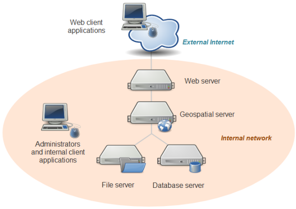
At the top is a drawing of a computer with the label: Web client applications. The computer image extends into a little cloud with the label: External Internet.
A line extends from the bottom of this cloud into a wide oval diagram with the label: Internal network. The line leads to the drawing of a Web server and then, below the Web server, to a Geospatial server. The line then branches to drawings of a file server (left) and a database server (right). To the left (within the Internal network oval) is another computer drawing with the label: Administrators and internal client applications.
For example, you might have:
- desktop workstations that are used by administrators and internal client applications. These machines will also be used to prepare data, author maps, and sometimes administer the other machines.
In this course, you will be using QGIS and some command line libraries such as GDAL to accomplish these tasks. GeoServer also has a web-browser-based administrator dashboard that you would use from this machine.
In some cases, your web map may be designed solely for the use of people within your organization and may never see the open web. In this scenario, client applications may also reside on these desktop workstation machines. - a database and/or file server holding all of your GIS data. This machine might be equipped with redundant storage mechanisms and regular backup scripts that prevent the loss of data.
In this course, you'll be using folders of shapefiles for some of the exercises. If you had decided to use a database like PostgreSQL or MariaDB, it would also go on this tier. - a geospatial web services server that has specialized software and processing power for drawing maps, responding to feature queries, and performing GIS analysis operations.
In this course, you will use GeoServer to host your web services. - a web server that acts as a web entry point into your organization's network. This is also called a proxy server. It is protected by firewalls that shield malicious traffic into your internal network. It's also a place where you can put web application code (such as HTML and JavaScript files) for your web maps.
In this course, you will just be using GeoServer on your local machine; therefore, you will not install separate web server software. GeoServer comes with an embedded “servlet” called Jetty that gives you a simple endpoint to your web services that you can locally access for testing. In a more formal setup where you wanted to reveal your GeoServer web services to the world, you would have a web server such as Apache that would forward requests to GeoServer.
In this course, you will put your web applications in your Jetty home folder (if the application uses GeoServer) or host them on Amazon's cloud storage (if your application does not use GeoServer). - many client applications that use the web map. These can be apps that run on your desktop workstation or they could be mobile apps. The clients may be based within your network, or you may allow them to come from outside your network. All clients must be able to make web requests through HTTP, and any client coming from outside your network must have an Internet connection.
This is the tier you usually have no control over; therefore, it's important to design for different browser versions, screen sizes, ambient lighting, and so forth.
In this course, you can use any modern web browser to test your apps and services. You can also use a mobile browser, such as Safari on the iPhone, to test the apps that you place on your personal webspace.
Again, when developing and testing a web map, you can certainly use a single physical machine to play all these roles. This is a common practice that keeps things simple and more economic. When you work for a “real world” company with its own network and are ready to deploy your web map, you will move your tested services and applications into a formal “production” environment where you have individual enterprise-grade machines for each role, as described above.
Elements of a web map
Building and using web maps is different from working with a desktop GIS for a variety of reasons:
- In a web map, any information you see has to be sent “across the wire” from the server to your browser, introducing latency.
- In a web map, you may be pulling in information from several different servers. Your map performance is therefore limited by the availability and speed of all the servers you're using.
- In a web map, performance may be affected by other people using the server at the same time.
- In a web map, you are limited to the display technologies supported by the client application, which may be a basic web browser.
These considerations can sometimes take people by surprise. For example, if you've only used ArcMap or QGIS in the past, you may not be accustomed to thinking about broadband speeds or sharing the machine with other people.
By far, the biggest challenge for new web mappers is understanding the amount of data that is displayed in their maps and how to get all that information drawn on the screen of a web user in sub-second speeds. Many people who have worked with desktop GIS packages are accustomed to adding dozens (or even hundreds) of layers to the map and switching them on and off as needed. Your powerful desktop machine may be able to handle the drawing of this kind of map; however, performance will be unacceptably slow if you try to move the map directly to the web. The server requires precious time to iterate through all those layers, retrieve the data, draw it, and send the image back to the client.
To address this problem, most web maps break apart the layers into groups that are handled very differently. Layers whose sole purpose are to provide geographic context are grouped together and brought into the map as a single tiled basemap. In contrast, thematic layers (the layers that are the focus of the map) are brought in as one or more separate web services and placed on top of the basemap. You might additionally decide to include a set of interactive elements such as popups, charts, analysis tools, and so forth.
Let's take a closer look at these three things--basemaps, thematic layers, and interactive elements--to understand how each is created and displayed.
Basemaps
A basemap provides geographic context for your map. In other words, it is usually not the main reason people look at your map, but your map would be difficult to interpret without it. The most common basemaps you've used online are vector road maps and remotely sensed imagery.
Although a basemap may consist of many sublayers (such as roads, lakes, buildings, and so forth), these are often fused together into a rasterized set of tiled images and treated as a single layer in your web map. These tiled maps consist of often thousands or millions of predrawn images that are saved on the server and passed out to web browsers as people pan around the map. Lesson 5 will explain tiled maps in greater depth and give you a chance to make your own.
In the past couple of years, it has become fashionable in some applications for the server to send the basemap as chunks of vector coordinates, sometimes known as "vector tiles." Displaying the basemap as vectors instead of a rasterized map allows for more flexibility in visualization, such as being able to rotate the map while the labels stay right-side-up. You can see a vector basemap in action if you look at the Google Maps app on a smartphone.
Sometimes two tiled layers will work together to form a basemap. For example, you may have a tiled layer with aerial imagery and a second tiled layer with a vector road overlay that has been designed to go on top of the imagery. (In Google Maps, this appears when you check the Labels item). Keeping these two tilesets separate takes less disk space and makes it easier to update the imagery.
Thematic layers
Thematic layers (also known as business or operational layers) go on top of the basemap. They're the reason people are coming to visit your map. If placed on the basemap, they might not be of interest to everybody, but when placed on your focused web map, they are the main layer of interest. If your map is titled “Farmers markets in Philadelphia,” then farmers markets are your thematic layer. If your map is titled “Migration patterns of North American birds,” then the migration patterns are your thematic layer.
Like basemaps, thematic layers are sometimes displayed with tiles; however, this may not always be possible due to the rapidly changing nature of some data. For example, if you need to display the real time positions of police vans, you cannot rely on predrawn tiles and must use some other way to draw the data. There are various web services such as WMS (which you will learn about in Lesson 4) that are designed to draw maps on the fly in this way. You can use these for your thematic layers. Another option is to query the server for all the data and use the browser to draw it. This approach lends itself well to interactive elements such as popups and is described in Lesson 6.
Thematic layers work together with basemap layers to form an effective web map. Interestingly, the thematic layer is not always the top one. In a 2009 blog post (no longer online), Esri cartographer Charlie Frye described a “map sandwich” approach, wherein a thematic layer (which could be tiled or not) is placed in between two tiled basemap layers that give geographic context. The bottom layer has physiographic features and the top layer has labels and boundaries. This is the “bread.” The thematic layer in the middle is the “meat.” The Esri "Light Gray Canvas" basemap in ArcMap and ArcGIS Online uses this technique. FOSS technology definitely allows this approach as well.
Your map may include several thematic layers that you allow users to toggle on and off. To accomplish this, you can use a single web service with multiple sublayers, or multiple web services that each contain a single layer. However, to keep your app usable and relatively fast-performing, you should avoid including many thematic layers in your web map.
Try this
- Open your browser's web developer tools you used during the previous lesson and open the Network tab; then visit Bing maps [39] on your computer's web browser.
- Pan around and switch between the basemaps (drop-down menu at the top right), and note the different web request URLs displayed in the table. These will appear quickly as you interact with the website.
- Click a row representing a request, and then click the Response tab to see what came back from the request. If you see an image (try a couple of the requests going to https://t.ssl.ak.dynamic.tiles.virtualearth.net [40] for this), it means the request sent back a tiled map image as a response. Other times you may see JSON and/or other text.
- Now turn on the thematic layer for Traffic.
How is Bing displaying these layers? Why are they taking this approach? At the end of this class, you will have a good understanding of the different options that exist and their advantages and disadvantages. Feel free to go ahead and check out HERE WeGo [41] in the same way (layer options can be accessed at the bottom right). You should notice a couple of similarities between the two web maps.
Interactive elements
Web maps are often equipped with interactive elements that can help you learn more about the layers in the map. These can be informational popups that appear when you click a feature, charts and graphs that are drawn in a separate part of the page, slider bars that adjust the time slice of data displayed in the map, and so forth. Some web maps allow you to edit GIS data in real time, or submit a geoprocessing job to the server and see the response drawn on the screen. Others allow you to type a series of stops and view driving directions between each.
These elements make the map come alive. The key to making an effective web map is to include the interactive elements that are most useful to your audience, without overwhelming them with options or making the tasks too complicated. Even a little bit of housekeeping, such as including user-friendly field aliases in your popups, can go a long way toward making your map approachable and useful.
Interactive elements are the part of your web map that require the most custom programming. The amount of interactivity you have the freedom to add may be strongly correlated with the amount of JavaScript programming that you know how to do. Open web mapping APIs such as OpenLayers and Leaflet provide convenient methods for doing some of the most common things, such as opening a popup.
Later in this lesson, you'll examine some web maps and discuss the interactive elements they provide. You'll also revisit this subject in Lesson 6 as you begin using the web mapping APIs to put all your layers together into a web map.
Getting some practice with identifying web map elements
Let's get some practice identifying these elements. I will walk you through two simple web maps and point out the basemap, the thematic layers, and the interactive elements. Then, in this week's assignment, you'll get the chance to try it yourself using two web maps of your choosing.
GDACS Disaster Alerts
The first map we'll look at is www.gdacs.org/ [44], published by the Global Disaster Alert and Coordination System (GDACS), a cooperation framework between the United Nations, the European Commission, and others to share disaster information and alerts. The web map on the main page showing alerts for the last four days is relatively simple in terms of interactive elements, focusing on displaying disaster related information and providing links to more detailed reports. This map has been created with OpenLayers. It is similar in scope to what you will be creating in this course. Take a minute to open this map and examine it.
- The map offers three different terrain-based basemap options serving as unintrusive backdrops for displaying the thematic layers. However, when you zoom in, you will see that at a certain zoom level the basemap changes to a typical road map version, similar to what you are familiar with from Google Maps, Bing, or OpenStreetMap. By inspecting the network traffic in the browser's network log while panning around and zooming, we can see that all these basemaps options are loaded as image tiles using URLs like this one:
https://gisco-services.ec.europa.eu/maps/tiles/NaturalEarth/EPSG3857/2/0/3.png
- The map has a larger number of thematic layers, most of them for displaying disasters of different types (fire, drought, flood, etc.) as icons/symbols on the map. When you zoom in, you will see that in addition to the icons there are actually vector features like polygons representing the events (including detailed past and predicted trajectories for cyclones). In addition, there are raster layers for rain and clouds. These two thematic layers are relatively easy to find in the browser's network log because they are also brought in as image tiles, in this case from a local ArcGIS Server installation using URLs like this one:
https://www.gdacs.org/arcgis/rest/services/GDACS/daily_rain/MapServer/export?F=image&FORMAT=PNG32&TRANSPARENT=true&SIZE=256%2C256&BBOX=-180%2C-90%2C-90%2C0&BBOXSR=4326&IMAGESR=4326&DPI=90
In contrast, to the previous URL for the basemap tiles, which used nested folders for zoom level, x and y coordinates of the tiles, we here find bounding box coordinates and other information encoded as arguments following the '?' which are then decoded by the server and used to produce the requested tile image. How about the other thematic layers? It turns out these do not come as images but fortunately, they can still be identified relatively easily in the network log because the URLs for the requests contain abbreviations for the event types, like this:https://www.gdacs.org/gdacsapi/api/events/geteventlist/MAP?eventtypes=EQ
These requests are sent out immediately when the map is loaded, and the response from the GDACS server always is a GeoJSON file with a text specification of the vector features and their geometries. These vector features are then drawn by the web browser. You will learn more about client-side rendering of data from GeoJSON files in Lesson 7. - The interactive elements of the map are a couple of buttons for zooming (top left), for accessing the layer switch control and legend for the Rain layer (top right), and for displaying some general information and attribution (bottom right) confirming that OpenStreetMap data has been used to create the map. Clicking on a symbol from one of the thematic layers will open a popup with information on the event and a link to the full report. When you add interactive elements to your web maps, you will often add code that "listens" for particular events, such as clicking, tapping, or hovering over a feature.
NYC Crime Map
The second map is a web map at https://maps.nyc.gov/crime/ [45] showing the concentration of crimes of different types for New York City. The map is entirely based on services provided by ESRI. The map is created in Javascript using ESRI's ArcGIS Javascript API and some other Javascript libraries for the general layout of the page such as Dojo..
- The basemap is tiled and the tiles are loaded from an arcgis.com using URLs of the following form:
https://tiles.arcgis.com/tiles/yG5s3afENB5iO9fj/arcgis/rest/services/NYC_Basemap/VectorTileServer/tile/14/6161/4830.pbf
Similar to the previous web map example, the tiles are stored on the server in some folder/file organization with numbers referring to the zoom level (.../14/...), x grid coordinate (.../6161/...), and y grid coordiante (.../4830.pbf). However, one important difference is that these are not image tiles. They are vector tiles using the .pbf vector tile format in which the content of the tile is specified as vector data that then still needs to be rendered by the web map application running in the browser when the .pbf file is received. Therefore, we don't get to see an image in the Preview of the browser's Developer Tools but rather some cryptic text because the .pbf file stores the vector data in binary format. Looking at the map itself, we can see that these basemap vector tiles are rendred using a light non-intrusive design. - There are two types of thematic layers that you can switch between under "Layers" at the top right. The polygon based , choropleth-style "Crimes by police precinct" layer and the point based "Crimes by location" layer that uses a cluster rendering approach with clusters of points represented by circles that then get split up when you zoom in further. These layers are also brought in as vector data and then rendered by the browser. Here is one example URL:
https://services6.arcgis.com/yG5s3afENB5iO9fj/arcgis/rest/services/NYC_Crime_Locations_PROD_view/FeatureServer/0/query?f=pbf&cacheHint=true&maxRecordCountFactor=4&resultOffset=8000&resultRecordCount=8000&where=1%3D1&orderByFields=OBJECTID&outFields=OBJECTID&outSR=102100&spatialRel=esriSpatialRelIntersects
We see that the data is coming from arcgis.com as well. We don't have to worry about the details of these requests for now but note how the details of what exactly is requested are encoded in the URL using different parameters separated by & symbols. - In addition to the standard map controls and the controls for choosing the layer and different information to be displayed in the area directly to the right of the map, the interactive elements of the web map allow for filtering the data presented in the thematic layers based on crime type and a date range. Clicking on one of the thematic features from either layer, will display more detailed information about that feature using visually appealing tables and interactive plots. You can also search for a particular location.
Other maps
Here are a few other maps you can look at if you want to keep practicing. Although some of these maps have very nice elements, I am recommending them for their variety, not for their excellence in any particular realm.
- TriMet Trip Ride Planner [47]
- Downtown Alliance Interactive Map New York [48] (click on Open Map View at the bottom right)
- NIU Campus Webmap [49]
From this brief exercise, you can begin to see the various approaches that can be used to put together a web map. Hopefully, you can look at a web map and immediately begin to see how the layers were broken up into basemap layers and thematic layers. Whenever you see a web map, you should also think about the interactive elements that are present and decide whether they are usable and applicable.
Walkthrough: Setting up GeoServer
GeoServer is free and open source software (FOSS) that exposes your data as geospatial web services. You'll be using GeoServer later in this course and possibly in your term project if you choose. This week, we'll take some time to get GeoServer installed and configured. This is a detour from our discussion of web map elements, but you'll soon revisit that topic in the weekly assignment.
Again, the lesson materials provide instructions for Windows. You are welcome to install on another platform, but you are on your own for instructions and troubleshooting.
- If you do not already have Java 8 on your computer, visit the Java download page [50] and install the latest version of Java 8. Make note of the file system location where you install it. You will need this when you set up GeoServer. In case that a new Java version will be released during the course and your computer asks you whether it should install the update. Be warned that if you decide to do so, GeoServer may stop working until you adapt the Java path in the GeoServer startup .bat file. Also, it is important that this is a version of Java 8; GeoServer most likely won't run with Java 9 or higher.
- Visit the GeoServer home page at www.geoserver.org [51] and click the Download link. From here you can download different versions of GeoServer including the most current stable and maintenance releases. You are free to check out these newer versions (it's pretty easy to work with multiple version of GeoServer on the same computer). If you want to play it safe and use the latest version we tested the course materials with, then follow the instructions in the next step to download version 2.19.6. The differences between these versions are minimal in the context of this class. If you decide to use a different version, make sure that you download the "Platform Independent Binary".
- To download GeoServer 2.19.6, click on this direct link [52] to start the download of the "Platform Independent Binary" from SourceForge.
- After the download has finished, you will have a .zip file called geoserver-x-y-z-bin.zip on your computer. Extract the content of this file to a new subfolder somewhere on your computer where you have read/write access, for instance in your user's home directory. The result should look similar to the screenshot below.
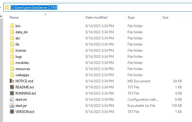 Figure 2.1b GeoServer installation folder after extracting the .zip file.
 - Now look in the subfolder called "bin". There you will find two .bat files for starting and shutting down GeoServer on Windows. These scripts will look for three important environment variables on your system: JAVA_HOME, GEOSERVER_HOME, and GEOSERVER_DATA_DIR. JAVA_HOME should point to your Java installation from step 1 above and should be set automatically. The other two need to refer to the new folder to which you just extracted the GeoServer file tree and to the subfolder called data_dir in it, which is meant for storing the spatial and other data to use with GeoServer. We could now go to the Windows Settings and define these environmental variables there, but instead we are going to define them in the script files themselves. This way, there won't be any issues with older GeoServer installations you may already have on your computer, and you will be able to simply delete the GeoServer folder at the end of the class if you want. So please open the file "startup.bat" in a text editor (make sure it is startup.bat, not startup.sh!) and add the following two lines at the very beginning. Adapt the path to the right of the equal sign in the first line to refer to your GeoServer folder.
set GEOSERVER_HOME=C:\Users\jow\GeoServer 2.19.6
set GEOSERVER_DATA_DIR=%GEOSERVER_HOME%\data_dir
Now do the same for the file called "shutdown.bat". - Now double-click startup.bat to start Geoserver.
You'll see a bunch of status messages appearing in a black and white console, like the following.
Wait a second for the messages to stop appearing, then go on to the next step. (If you keep this window open, you'll see messages appear as you interact with GeoServer. This is okay, and may even help you with troubleshooting.) Figure 2.2 Status messages during GeoServer startup.
If you get a Windows Security Alert that Windows Firewall has blocked some features of the program, check the top box to allow it to run on private networks and click Allow access. Uncheck the bottom box, as public access will not be needed in this course. - Next, go to your browser and enter the address localhost:8080/geoserver/web.
This is a web page that you can use to administer GeoServer from this or any other computer in your network. You might be wondering, "How did my machine get the ability to serve out web pages?" This is possible because GeoServer includes a servlet [54] called Jetty, which allows your machine to respond to web service and web page requests without having a full-blown web server software package installed.
In an enterprise environment, you would install GeoServer onto your existing web server such as Apache Tomcat, and it is very possible that you will need to do this sometime in the future. The process is straightforward enough that I was able to do it following this instructional YouTube video [55] even though the video is not in English; however, for the assignments in this class, please use the Jetty server and only attempt the Tomcat install if Jetty is not working. My intent is to keep everyone on as close to the same environment as possible, so that I can be more helpful with troubleshooting if needed. - Log into GeoServer by using the username admin and the password geoserver in the upper boxes and click Login. These are the default username and password for the administrator account. You must use this the first time you log in.
You will see a welcome page similar to the following:
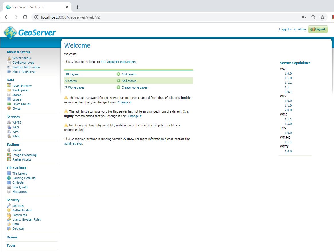 Figure 2.3 Geoserver startup webpage
 - Rather than working with files that represent an entire map, like .mxd or .qgs, GeoServer works with the concept of layers and layer groups. You define a set of datasets that you want to have exposed on your server, and then you define what characteristics they'll exhibit when brought into web maps as web service layers.
GeoServer comes with a bunch of sample layers already loaded. Let's take a look at those. - In the left-hand menu, click Layer Preview.
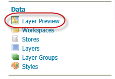 Figure 2.4 Layer Preview
 - Scroll down to the Tasmania state boundaries layer and click the OpenLayers link.
This displays your map as a web service that you can navigate. The web service was delivered through the Open Geospatial Consortium (OGC) Web Map Service (WMS) specification, an openly documented way of serving web maps that you'll learn more about in Lesson 4. The map frame and navigation buttons were created through the OpenLayers JavaScript framework.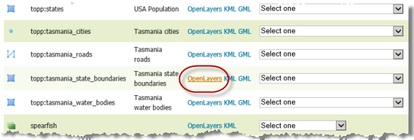 Figure 2.5 Find Tasmania in the list of layers
It's important to understand that you also could have done this by clicking the dropdown list and choosing WMS > OpenLayers 3 (or just OpenLayers on older versions of GeoSever). Looking at this list, you get a better idea of the many different output formats supported by GeoServer.Let's try one of these other options.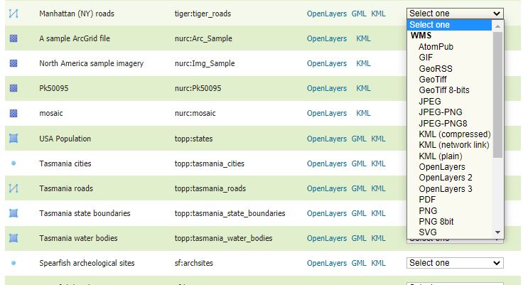 Figure 2.6 OpenLayers selection in GeoServer
 - Close the map preview window and return to the GeoServer layer preview list. This time, click the KML link to get the layer as KML and XML-based open specification for geographic data, often used by Google. If you have Google Earth installed, the layer should open there. If you don't have Google Earth, you can open the downloaded .kml file in Notepad and just examine the raw KML.
In addition to requesting many layer formats, you can request groups of layers together if they have been configured as a group layer. GeoServer comes with a few preconfigured group layers. - In the GeoServer layer preview list, scroll down to the Tasmania group layer (symbolized by green squares). Using the techniques you have learned, preview this in OpenLayers.
Here, you see three layers that have been delivered together as one map.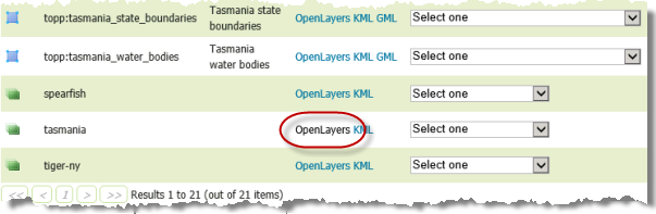 Figure 2.7 Layer preview in GeoServer
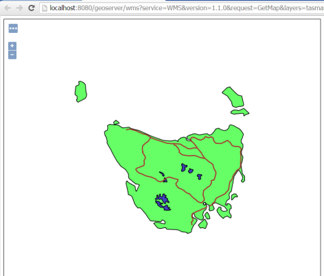 Figure 2.8 Preview of Tasmania from GeoServer
You'll return to GeoServer later in this course. This walkthrough just ensures you have it up and running correctly. If technical difficulties prevented you from getting to this point, please alert your instructor.
Lesson 2 assignment: Analyze two web maps
For this week's assignment, find two web maps "in the wild" and create a post on the "Lesson 2 assignment forum" on Canvas that describes the following for each map:
- The web address (URL) of the map and who created it.
- The basemap, thematic layers, and interactive elements in the map.
- The servers and display techniques used for each layer (tiles, image drawn by the server on the fly, browser-drawn vector graphics, etc.). Use your web browser's developer tools/plugins to figure this out. For example, using the Network tab of the developer tools while you pan around the map, you might determine that your web map is pulling in a tiled basemap from CloudMade.com. This is enough for the assignment; you don't have to go into further technical details about how the tiles were made or their file structure.
- The software and programming framework used to build the web map (if you can determine this) and whether it is proprietary or FOSS.
- Suggestions on how the map administrator could make this map more useful or faster performing.
Please make an effort to find these maps on your own. In other words, do not choose any of the web maps previously referenced in this lesson, nor should you browse through other students' posts in order to find maps to analyze. Except for the first point (URL), please use short paragraphs to address the different points in your description similar to what you saw in this lesson, not just bullet point enumerations.
If you are having difficulties analyzing your web map, please refer back to the section "Elements of a web map" and the examples and techniques using your browser's developer tool described there. If you check out the requests in the Network log, requests for images drawn by a server will be relatively easy to identify because the individual images sent back to the browser as a response will be image files in one of the typical image formats (.png, .jpg, etc.). You will be able to see images under 'Preview' of the Network tab. Looking at the preview images will allow you to identify which layers are included, e.g. is it just the basemap, just one thematic layer, or maybe basemap and thematic layer combined. Then the last question is whether these images are tiles, so are multiple images requested and then put together to cover the entire area of the map you are seeing, or is it always just a single image covering the entire map area (something that, for instance, you can experience with a WMS service where the browser tells the server the extent of the area covered by the map, the server then renders an image for that area and sends it back to the browser).
With requests for vector data that that is then rendered by the browser, things are more difficult. The vector data sent by the browser can come in a variety of formats (.json and .pbf are common ones) and is often in a binary format or in some other way compressed, in which case there is no direct way to check out what exactly the files contain. So if you come to the conclusion that some of the data for your map is not coming in as images, that's goood enough for this assignment. If you are able to identify some candidate requests in the network, you should mention that and the server these are going to, but in some cases even that can be difficult, e.g. when the vector data is just stored in a local file on the same web server that is hosting the page with the map.
Term project introduction
This course contains many walkthroughs showing how to use FOSS, but the ultimate objective is to apply these skills toward your own web map using data that's interesting to you (or your supervisor at work!). As the course progresses, you'll be expected to complete a portion of the weekly assignments using your own datasets. By the end of the course, this will become a fully functioning "term project" web map that combines base layers, thematic layers, and some degree of interactivity through popups, filters, or queries.
Part of the final week of the course is reserved for putting the finishing touches on your term project; however, most of the major pieces will be in place by that time if you put a respectable effort into the weekly walkthroughs and assignments.
Proposing an idea for the term project
Please do the following to get started with the term project:
- Skim through the upcoming lesson pages and titles to get an idea for the functionality that will be covered in this course. This will help you choose a project that is within scope.
- Read the Term project submission guidelines [56] to see what you will be required to submit
- Create a 1 - 2 paragraph write-up describing an idea for your term project. This should mention the basemaps, thematic layers, and interactive elements that you'd like to have in your project, along with an explanation of where you will get the data. Place this in the Term Project Proposal drop box on Canvas, which you can find by going "Modules tab" -> "Lesson 2" -> "Term project proposal drop box". We will reply within a week, commenting on the scope and appropriateness of the project.
Lesson 3: Storing and processing spatial data with FOSS
The links below provide an outline of the material for this lesson. Be sure to carefully read through the entire lesson before returning to Canvas to submit your assignments.
Note: You can print the entire lesson by clicking on the "Print" link above.
Overview
Underneath any web map are spatial datasets representing the entities to be placed on the map and their various attributes. In this lesson, you will learn about FOSS options for storing and processing spatial data. The broad scope of this course prohibits a full discussion of database theory and design; however, you will hopefully learn enough to select the appropriate type of data format for your project. Once you get your data in order, you'll be ready to launch GIS web services and assemble them into a web map.
Objectives
- List common open formats for spatial data and give appropriate uses for each.
- Recognize the advantages of various data storage architectures and formats.
- Process (clip and project) GIS data using QGIS and GDAL, and describe when it would be appropriate to use each.
- Experiment with a new GDAL function and use the documentation to learn how to invoke it.
Checklist
- Read the Lesson 3 materials on this page.
- Complete the two walkthroughs.
- Complete the Lesson 3 assignment.
- Complete the "First quiz" on Canvas. This covers material from Lessons 1 - 3.
Some common open formats for spatial data
This section of the lesson describes in greater detail some of the spatial data formats that have open specifications or are created by open source software. Note that these refer to files or databases that can stand alone on your hardware. We will cover open formats of web services streamed in from other computers in future lessons.
File-based data
File-based data includes shapefiles, KML files, GeoJSON, and many other types of text-based files. Each of the vector formats has some mechanism of storing the geometry (i.e., vertex coordinates) and attributes of each feature. Some of the formats, such as KML may also store styling information.
Below are some of the file-based data formats you're most likely to encounter.
Shapefiles
The Esri shapefile is one of the most common formats for exchanging vector data. It actually consists of several files with the same root name, but with different suffixes. At a minimum, you must include the .shp, .shx, and .dbf files. Other files may be included in addition to these three when extra spatial index or projection information is included with the file. This ArcGIS Resources article [57] gives a quick overview of the different files that can be included.
Because a shapefile requires multiple files, it is often expected that you will zip them all together in a single file when downloading, uploading, and emailing them.
If you want to make a shapefile from scratch, you can refer to the specification from Esri [58]. This is not for the novice programmer, and browsing this spec will hopefully increase your appreciation for those who donate their time and skills to coding FOSS GIS programs.
GeoPackages
The GeoPackage [59] is a relatively new format for storing and transferring vector features, tables, and rasterized tiles across a variety of devices, including laptops, mobile devices, and so forth. It was defined by the Open Geospatial Consortium (OGC), a group you will learn about in more detail in Lesson 4 that consists of industry representatives, academics, practitioners, and others with an interest in open geospatial data formats. The GeoPackage actually stores the data in a SQLite database, described below in more detail in the databases section. I list the GeoPackage here in the file-based formats section because some have advocated [60] for its adoption as a more modern alternative to the shapefile.
KML
KML gained widespread use as the simple spatial data format used to place geographic data on top of Google Earth. It is also supported in Google Maps and various non-Google products.
KML stands for Keyhole Markup Language, and was developed by Keyhole, Inc., before the company's acquisition by Google. KML became an Open Geospatial Consortium (OGC) standard data format in 2008, having been voluntarily submitted by Google.
KML is a form of XML, wherein data is maintained in a series of structured tags. At the time of this writing, the Wikipedia article for KML [61] contains a simple example of this XML structure. KML is unique and versatile in that it can contain styling information, and it can hold either vector or raster formats ("overlays", in KML-speak). The rasters themselves are not written in the KML, but are included with it in a zipped file called a KMZ. Large vector datasets are also commonly compressed into KMZs.
GeoJSON and TopoJSON
JavaScript Object Notation (JSON) is a structured means of arranging data in a hierarchical series of key-value pairs that a program can read. (It's not required for the program to be written in JavaScript.) JSON is less verbose than XML and ultimately results in less of a "payload," or data size, being transferred across the wire in web applications.
Following this pattern, GeoJSON is a form of JSON developed for representing vector features. The GeoJSON spec [62] gives some basic examples of how different entities such as point, lines, and polygons are structured.
You might choose to save GeoJSON features into a .js (JavaScript) file that can be referenced by your web map. Other times, you may encounter web services that return GeoJSON.
A variation on GeoJSON is TopoJSON [63], which stores each line segment as a single arc that can be referenced multiple times by different polygons. In other words, when two features share a border, the vertices are only stored once. This results in a more compact file, which can pay performance dividends when the data needs to be transferred from server to client.
Other text files
Many GIS programs can read vector data out of other types of text files, such as .gpx (popular format for GPS tracks) and various types of .csv (comma-separated value files often used with Microsoft Excel) that include longitude (X) and latitude (Y) columns. You can engineer your web map to parse and read these files, or you may want to use your scripting skills to get the data into another standard format before deploying it in your web map. This is where Python skills and helper libraries can be handy.
Various raster formats
Most raster formats are openly documented and do not require royalties or attribution. These include JPEG, PNG, TIFF, BMP, and others. The GIF format previously used a patented compression format, but those patents have expired.
Web service maps such as WMS return their results in raster formats, as do many tiled maps. A KML/KMZ file can also reference a series of rasters called overlays.
Spatially-enabled databases
When your datasets get large or complex, it makes sense to move them into a database. This often makes it easier to run advanced queries, set up relationships between datasets, and manage edits to the data. It can also improve performance, boost security, and introduce tools for performing spatial operations.
Below are described several popular approaches for putting spatial data into FOSS databases. Examples of proprietary equivalents include Microsoft SQL Server, Oracle Spatial, and the Esri ArcSDE middleware (packaged as an option with ArcGIS Enterprise) that can connect to various flavors of databases, including FOSS ones.
PostGIS
PostGIS is an extension that allows spatial data management and processing within PostgreSQL (often pronounced "Postgress" or "Postgress SQL"). PostgreSQL is perhaps the most fully featured FOSS relational database management system (RDBMS). If a traditional RDBMS with relational tables is your bread and butter, then PostgreSQL and PostGIS are a natural fit if you are moving to FOSS. The installation is relatively straightforward: in the latest PostgreSQL setup programs for Windows, you just check a box after installation indicating that you want to add PostGIS. An importer wizard allows you to load your shapefiles into PostGIS to get started. The rest of the administration can be done from the pgAdmin GUI program that is used to administer PostgreSQL.
Most FOSS GIS programs give you an interface for connecting to your PostGIS data. For example, in QGIS you might have noticed the button Add PostGIS Layers  . The elephant in the icon is a symbol related to PostgreSQL. GeoServer also supports layers from PostGIS.
This course, Geog 585, does not provide walkthroughs for PostGIS; however, there are a couple of excellent open courseware lessons in Geog 868: Spatial Databases [64] that describe how to install and work with PostGIS. I encourage you to make time to study these on your own (or take the instructor-led offering) if you feel that learning PostGIS will be helpful in your career.
You are welcome to use PostGIS in your term project if you feel comfortable with the other course material and want to take on an additional challenge. You can always fall back on file-based data if an excessive amount of troubleshooting is required.
SpatiaLite
SpatiaLite is an extension supporting spatial data in the SQLite database. As its name indicates, SQLite is a lightweight database engine that gives you a way to store and use data in a database paradigm without installing any RDBMS software on the client machine. This makes SQLite databases easy to copy around and allows them to run on many kinds of devices. If you are familiar with Esri products, a SpatiaLite database might be thought of as similar to a file geodatabase.
SpatiaLite is not as mature as PostGIS, but it is growing in popularity, and you will see a button in QGIS called Add SpatiaLite Layer  . If you feel it would be helpful in your career, you are welcome to use SpatiaLite in your term project. If you choose to do this, I ask you to first get the project working with file-based data. Then feel free to experiment with swapping out the data source to SpatiaLite.
You will encounter a SpatiaLite database in the Lesson 9 walkthrough when you use QGIS to import data from OpenStreetMap. In that scenario, you are dealing with a large amount of data with potentially many fields of complex attributes. SpatiaLite is a more self-contained and flexible choice than shapefiles, KML, etc., for this type of task.
The Data Tier Of Your Web Mapping Architecture
In the previous lesson, you learned that system architectures for web mapping include a data tier. This could be as simple as several shapefiles sitting in a folder on your server machine, or it could be as complex as several enterprise-grade servers housing an ecosystem of standalone files and relational databases. Indeed, in our system architecture diagram, I have represented the data tier as containing a file server and a database server.
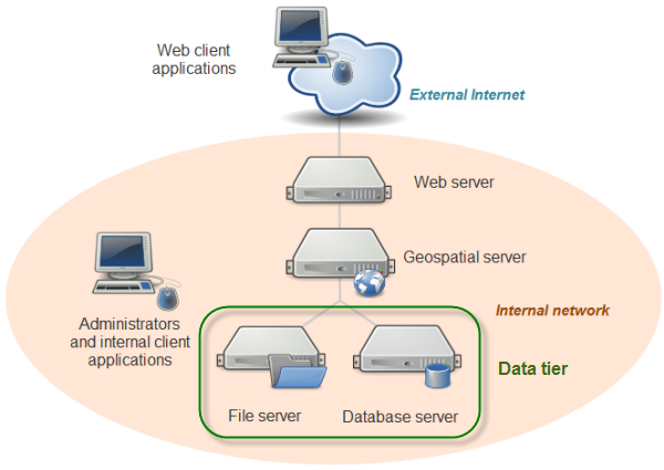
The data tier contains your datasets that will be included in the web map. Almost certainly, it will house the data for your thematic web map layers. It may also hold the data for your basemap layers, if you decide to create your own basemap and tile sets. Other times, you will pull in basemaps, and quite possibly some thematic layers, from other peoples' servers, relieving yourself of the burden of maintaining the data.
Some organizations are uneasy with the idea of taking the same database that they use for day-to-day editing and putting it on the web. There is justification for this uneasiness, for both security and performance reasons. If you are allowing web map users to modify items in the database, you want to avoid the possibility of your data being deleted, corrupted, or sabotaged. Also, you don't want web users' activities to tax the database so intensely that performance becomes slow for your own internal GIS users, and vice versa.
For these reasons, organizations will often create a copy or replica of their database and designate it solely for web use. If features in the web map are not designed to be edited by end users, this copy of the database is read-only. If, on the other hand, web users will be making edits to the database, it is periodically synchronized with the internal "production" database using automated scripts or web services. A quality assurance (QA) step can be inserted before synchronization if you would prefer for a GIS analyst to examine the web edits before committing them to the production database.
Where to put the data? On the server or its own machine?
You can generally increase web map performance by minimizing the number of "hops" between machines that your data has to take before it reaches the end user. If your data is file-based or is stored in a very simple database, you may just be able to store a copy of it directly on the machine that hosts your geospatial web services, thereby eliminating network traffic between the geospatial server and a data server. However, if you have a large amount of data, or a database with a large number of users, it may be best to keep the database on its own machine. Isolating the database onto its own hardware allows you to use more focused backup and security processes, as well as redundant storage mechanisms to mitigate data loss and corruption. It also helps prevent the database and the server competing for resources when either of these components is being accessed by many concurrent users.
If you choose to house your data on a machine separate from the server, you need to ensure that firewalls allow communication between the machines on all necessary ports. This may involve consulting your IT staff (bake them cookies, if necessary). You may also need to ensure that the system process running your web service is permitted to read the data from the other machine. Finally, you cannot use local paths such as C:\data\Japan to refer to the dataset; you must use the network name of the machine in a shared path; for example, \\dataserver\data\Japan.
Files vs. databases
When designing your data tier, you will need to decide whether to store your data in a series of simple files (such as shapefiles or KML) or in a database that incorporates spatial data support (such as PostGIS or SpatiaLite). A file-based data approach is simpler and easier to set up than a database if your datasets are not changing on a frequent basis and are of manageable size. File-based datasets can also be easier to transfer and share between users and machines.
Databases are more appropriate when you have a lot of data to store, the data is being edited frequently by different parties, you need to allow different tiers of security privileges, or you are maintaining relational tables to link datasets. Databases can also offer powerful native options for running SQL queries and calculating spatial relationships (such as intersections).
If you have a long-running GIS project housed in a database, and you just now decided to expose it on the web, you'll need to decide whether to keep the data in the database or extract copies of the data into file-based datasets.
Open data formats and proprietary formats
To review a key point from the previous section, in this course, we will be using open data formats, in other words, formats that are openly documented and have no legal restrictions or royalty requirements on their creation and use by any software package. You are likely familiar with many of these, such as shapefiles, KML files, JPEGs, and so forth. In contrast, proprietary data formats are created by a particular software vendor and are either undocumented or cannot legally be created from scratch or extended by any other developer. The Esri file geodatabase is an example of a well-known proprietary format. Although Esri has released an API for creating file geodatabases, the underlying format cannot be extended or reverse engineered.
Some of the most widely-used open data formats were actually designed by proprietary software vendors, who made the deliberate decision to release them as open formats. Two examples are the Esri shapefile and the Adobe PDF. Although opening a data format introduces the risk that FOSS alternatives will compete with the vendor's functionality, it increases the interoperability of the vendor's software, and, if uptake is widespread, augments the vendor's clout and credibility within the software community.
Processing spatial data with FOSS
Imagine you've identified some spatial data to use in your web map, but the data doesn't quite fit your purposes yet. It covers a broader region than your study area, and you want it to be in a different projection. Maybe you have a raster DEM that you need to convert into a hillshade, or perhaps you want to interpolate some raster surfaces that you can use in a time series animation. Indeed, a large portion of your datasets will probably need some kind of preprocessing before you incorporate them into your web map.
In these situations, you need to:
- identify the FOSS tools that can help you do the data processing;
- learn how to use the tools successfully;
- take notes on what you did so that you remember how to do it in the future!
If you're accustomed to a proprietary GIS software package that contains hundreds of tools and uniform documentation out of the box, it may seem frustrating to move to FOSS. Cobbling together a range of tools and collecting bits or pieces of documentation may seem like a waste of precious time. This is the tradeoff that you make when you use free software. Fortunately, the number of operations to learn is finite, and most of the time you'll probably be doing one of a dozen or fewer common actions, such as selecting data, projecting, clipping, and buffering. After you've learned how to do these once, you can go back and repeat the steps with any dataset, especially if you have taken good notes. Also, scripting these actions or running them in batch may require less overhead and processing time than you experience with proprietary software.
This is not a course about spatial data processing; however, this particular lesson attempts to give you some experience doing data processing with FOSS. You will learn a few resources for addressing data processing, and you'll get a feel for how to approach new tools.
Tools you will use in this course for data processing
In this course, you'll use QGIS and its associated plugins as a GUI tool for data processing. You will also learn how to use the GDAL and OGR command line utilities. These are explained in more detail below.
QGIS
QGIS offers a lot of the most common vector and raster processing tools out of the box. Additionally, developers in the QGIS user community have contributed plugins that can extend QGIS functionality.
Open QGIS and explore the Vector menu to see some of the operations for processing vector data. You'll notice tools for merging, summarizing, intersecting, buffering, clipping, and more.
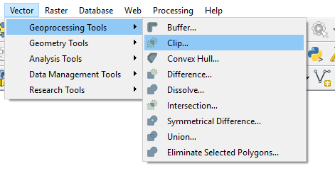
Some of the most powerful options are hidden in the Export context menu item when you right-click a vector layer. The Save Features As... dialog box allows you to convert data between different formats (for example, convert a shapefile to GeoJSON) and reproject the data to a new coordinate system.
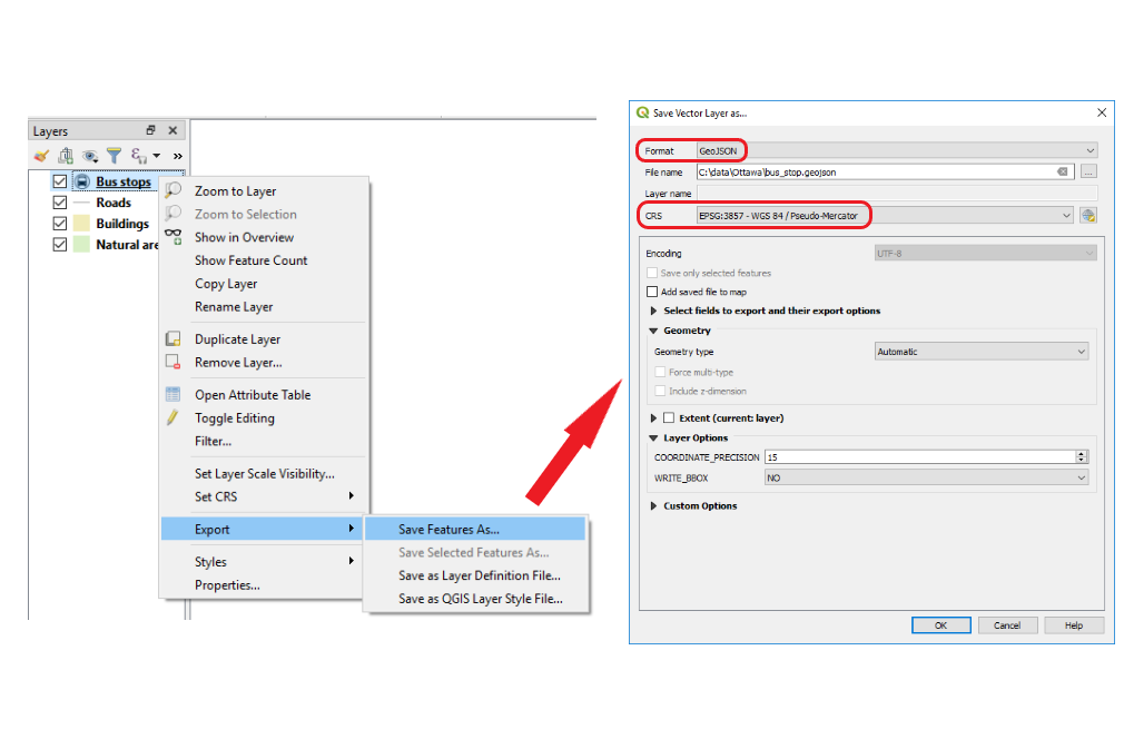
Now, go back up to the top of the QGIS screen and click the Raster menu to see some of the options for processing rasters. Notice that you can warp, clip, contour, and interpolate to raster formats, along with various other operations.
In addition to these common vector and raster processing options, the Processing > Toolbox menu at the top of the QGIS screen gives you a dockable side window with access to many additional functions, some of them more obscure than others. This toolbox is akin to the full "ArcToolbox" that you see in Esri software. One difference is that it contains tools from multiple software packages, including GDAL, GRASS, and SAGA (a popular open source library for processing rasters). One of the more common "algorithms" (as they are called in QGIS) that I use in this toolbox is Create Grid, which can create square or hexagon lattices for cartographic "binning" or, in other words, aggregation to uniformly shaped regions in order to get a better visualization of a point pattern. Creating a lattice of hexagons is a task not easy to do by hand, and is well-suited to a pre-canned tool.
If you don't see what you're looking for in any of the above locations, someone may have developed a plugin for it. QGIS comes with a few of the more useful plugins already installed. Click Plugins > Manage And Install Plugins to see what they are. Here, you can disable some of these plugins if you don't like them getting in the way.
If you want to add more plugins, you can do it directly from this dialog box by clicking Not installed. Do this now, and examine the descriptions of some of the plugins you can add (the list may vary from what you see below).

You can even pick one and install it if you like. The OpenLayers plugin shown above is a handy way to see OpenStreetMap, Google Maps, etc. in QGIS. This plugin is still declared "experimental" in QGIS 3, so most likely you will only be able to see the plugin if you first click on the Settings tab and select the option to show experimental plugins. The plugin will add a new entry in the Web menu, from which you can pick different basemap options. Be aware that the quality and usability of the plugins may vary.
GDAL and OGR utilities
Many spatial data processing functions use well-known logic or documented algorithms. It would cause extra tedious work and possibly introduce errors and inconsistency if every FOSS developer had to code these same operations from scratch. Therefore, many FOSS programs take advantage of a single open source code library called GDAL (Geospatial Data Abstraction Library) to perform the most common functions.
GDAL is most commonly thought of as a raster processing library. But within GDAL is an important repository of vector processing functions called the OGR Simple Features Library. You will hear the terms GDAL and OGR many times as you work with FOSS, so get used to them. You can thank a man named Frank Warmerdam for initiating and maintaining these libraries over time. Although you may have never heard of him, you've probably done something to run his code at one point or another.
One way to use GDAL and OGR is by launching functions from QGIS or some other GUI-based program, like you would get from the menu options pictured above. Another way is to write code in Python, C#, or some other language that calls directly into these libraries. A third way, which lies in the middle in terms of complexity and flexibility, is to call into GDAL and OGR using command line utilities. These utilities were installed for you when you installed QGIS. You will get a feel for them in the lesson walkthrough.
Other tools
There are many other FOSS tools out there for wrangling spatial data; new ones appear all the time. Later in this course you'll be required to find one, test it out, review it, and share it with the class. Be an explorer, and if you find something that works for you, stick with it. You can certainly use any FOSS tool that works for you in order to complete the term project.
Walkthrough: Clipping and projecting vector data with QGIS and OGR
This walkthrough will first give you some experience using the GUI environment of QGIS to clip and project some vector data. Then, you'll learn how to do the same thing using the OGR command line utilities. The advantage of the command line utility is that you can easily run it in a loop to process an entire folder of data.
This project introduces some data for Philadelphia, Pennsylvania that we're going to use throughout the next few lessons. Most of these are simple basemap layers that I downloaded and extracted from OpenStreetMap; however, the city boundary is an official file from the City of Philadelphia that I downloaded from PASDA [66].
Download the Lesson 3 vector data [67]
Clipping and projecting data with QGIS
- Extract the dataset to a simple path such as C:\data\PhiladelphiaBaseLayers.
- Open the folder and explore it a bit. You'll see a bunch of shapefiles that you can add to QGIS and examine. Also, notice that I have created three folders in preparation for our exercise: clipFeature, clipped, and clippedAndProjected.
- These datasets use a geographic coordinate system and cover the large region of greater Philadelphia. Our processing task is to clip them to the Philadelphia city boundary, then project them into the modified Mercator coordinate system used by popular online web maps (like Google, Bing, Esri, and so forth).
- First, we'll clip and project a dataset using QGIS. This is an easy way to process a single dataset, especially if you're using a tool for the first time.
- Launch QGIS and add fuel.shp and clipFeature/city_limits.shp to the map.
- Click Vector > Geoprocessing Tools > Clip.
- Set the Input vector layer as fuel and the Clip layer as city_limits. Set the output shapefile to be saved in the subfolder as clipped/fuel.shp as shown below. You need to click the ... button, then choose Save to File... and select .SHP for the output format.
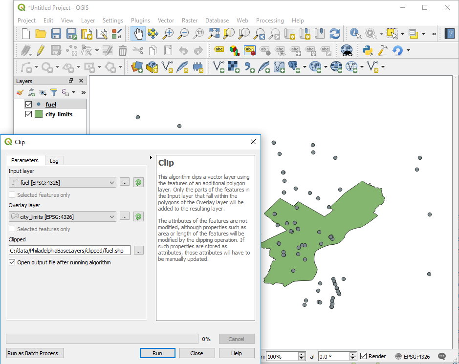 Figure 3.5 Clip tool GUI
 - Select the checkbox for adding the result to the canvas ("Open output file after running algorithm") so you can verify your work. Then click Run. The new layer should only contain features within the boundary of Philadelphia.
Now, let's project this dataset. In QGIS, you do this by saving out a new layer.
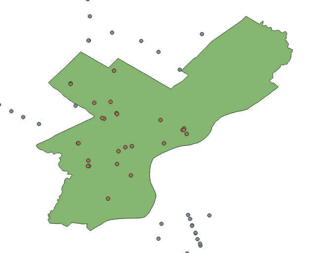 Figure 3.6 Clip tool results
 - In the table of contents, right-click the clipped fuel dataset (not the original one!) and click Export -> Save Features As.... Make sure that the Format box is set to ESRI Shapefile.
- Next to the File name box where you are prompted to put a path, click the ... button and set the path for the output dataset as clippedAndProjected/fuel.shp.
- Next to the CRS box, click the Select CRS button on the right. This is where you'll specify the output projection. The nice thing is that you can search.
- In the Filter box, type pseudo and select WGS 84 / Pseudo Mercator (EPSG: 3857) (not EPSG: 6871). Then click OK.
This projection has lots of names, and we'll cover more of its history in other lessons. For now, remember that you can recognize it using its EPSG code which should be 3857. (Most projections have EPSG codes to overcome naming conflicts and confusion).
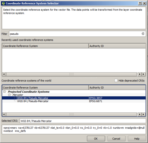 Figure 3.7 QGIS Coordinate reference system dialog
 - Click OK to save out the projected layer. A good way to verify it worked is to start a new map project and add it.
- Create a new map project in QGIS (there's no need to save the old one) and add the clippedAndProjected/fuel.shp file. The layout of the features should look something like what you see below. (I put an SVG marker symbol on this as in Lesson 1, just for fun.)
In QGIS, just like in ArcMap, the first layer you add to the map determines the projection. Notice how the EPSG code in the lower right corner is 3857, proving that my data was indeed projected. If you add any of our other layers to this map, make sure you add them after you add the fuel layer for this reason.
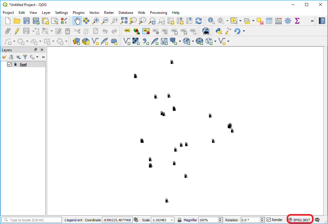 Figure 3.8 Sample QGIS layout showing updated map projection
Clipping and projecting data using the OGR command line utilities
That was easy enough, but it would be tedious, time-consuming, and possibly error prone if you had to do it for more than a few datasets at a time. Let's see how you could use the OGR command line utilities to do this in an automated fashion. Remember that OGR is the subset of the GDAL library that is concerned with vector data.
When you install QGIS, you also get some executable programs that can run GDAL and OGR functions from the command line. The easiest way to get started with these is to use the OSGeo4W shortcut that appeared on your desktop after you installed QGIS.
- Double-click the OSGeo4W shortcut on your desktop. If there's no shortcut, try Start > All Programs > QGIS > OSGeo4W Shell or simply search for OSGeo4W.
You should just see a black command window, possibly displaying some progress output from setting up GDAL and OGR.
We'll walk through the commands for processing one dataset first, then we'll look at how to loop through all files in a folder. For both of these tasks, we'll be using a utility called ogr2ogr. This utility processes an input vector dataset and gives you back a new output dataset (hence, the name). You will use it for both clipping and projecting.
OGR actually lets you do a clip and project in a single command, but, according to the documentation, the projection occurs first. For the sake of simplicity and performance, let's do the clip and the projection as separate actions. We'll do the clip first so we don't project unnecessary data. - Take a look at the documentation for OGR2OGR [68] and see if you can decipher how it's used. When you run this utility, you first supply some optional parameters, then you supply some required parameters. The first required parameter is the name of the output dataset. The second required parameter is the name of the input dataset. These are pretty basic required parameters, so a lot of the trick to using ogr2ogr is to set the optional parameters correctly depending on what you want to do.
- Type the following command in your OSGeo4W window, making sure you replace the paths with your own. Note that this is a single command line with the different parts separated by spaces, NOT multiple lines separated by linebreaks! Also, in case any folder names you use contain spaces, you will have to put the entire paths into double quotes (e.g. "c:\my data folder\PhiladelphiaBaseLayers\...\city_limits.shp").
ogr2ogr -skipfailures -clipsrc c:\data\PhiladelphiaBaseLayers\clipFeature\city_limits.shp c:\data\PhiladelphiaBaseLayers\clipped\roads.shp c:\data\PhiladelphiaBaseLayers\roads.shp
- Wait a few minutes for the command to run. You'll know it's done because you'll get your command prompt back (e.g., C:\>). If you get a failure, hit the up arrow key and your original command will reappear. Examine it to see if you made a typo.
- Open a new map in QGIS and add clipped\roads.shp to verify that the roads are clipped to the Philadelphia city limits.
Take a close look at the parameters you supplied in the command. You'll notice two optional parameters: --skipfailures (which does exactly what it says, and is useful with things like OpenStreetMap data when you can get strange topological events occurring) and --clipsrc (which represents the clip feature). The last two parameters are unnamed, but you can tell from the documentation that they represent the path of the output dataset and the path of the input dataset, respectively.
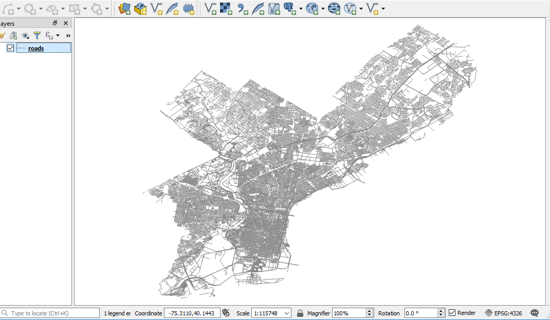 Figure 3.9 Sample QGIS map layout of Philadelphia roads
Now let's run the projection. - Type the following command (again this is a single command with the different parts separated by spaces):
ogr2ogr -t_srs EPSG:3857 -s_srs EPSG:4326 c:\data\PhiladelphiaBaseLayers\clippedAndProjected\roads.shp c:\data\PhiladelphiaBaseLayers\clipped\roads.shp
This one should run more quickly than the clip. - Start a new map in QGIS and add clippedAndProjected\roads.shp. It should be stretched a little more vertically than before.
Examining the parameters that you used for this command in tandem with the documentation, you'll notice that -s_srs is the coordinate system of the source dataset (EPSG:4326, or the WGS 1984 geographic coordinate system) and -t_srs is the target coordinate system (EPSG:3857, or the web Mercator projection). Because we're still using the ogr2ogr command, the final two parameters are the output and input dataset paths, respectively.
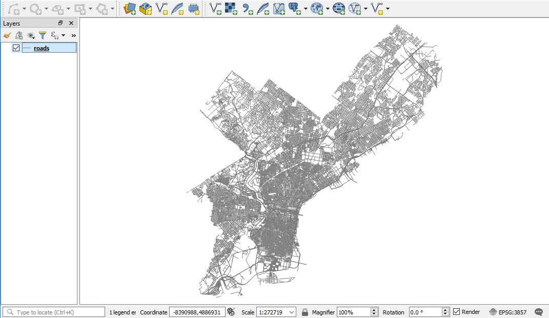 Figure 3.10 Sample QGIS map layout of Philadelphia roads in a different projection
You may be wondering, "How will I know which EPSG codes to use for the projections I need?" The easiest way to figure out the EPSG code for an existing dataset (which you'll need for the -s_srs parameter) is to add the dataset to a new map in QGIS and look in the lower-right corner of the screen as shown in Step 12 above. The easiest way to figure out the EPSG code for the target dataset (which you'll need for the -t_srs parameter) is to run the Save As command in QGIS and search for the projection. The EPSG code will appear as shown in Step 10 above.
Technical note for older versions of QGIS: If you are using a very, very old version of QGIS (prior to approximately version 2.14 Essen), you may see that the output dataset is shown in the Mercator projection, but the projection is reported in the lower-right hand corner as either EPSG:54004 or USER:100001 rather than EPSG:3857. In addition, if you add the original city_limits shapefile and the projected one to the same map project, you will notice a roughly 20km offset between the two polygons. QGIS needs a .qpj (QGIS projection file) to be associated with the shapefile in order to interpret the EPSG:3857 projection correctly. The ogr2ogr utility does not create the .qpj file by default because ogr2ogr is a general utility that is used with a lot of different programs, not just QGIS. To get a .qpj file, you could manually project a single dataset with QGIS into EPSG:3857, just like we did in the first set of steps above. This creates a shapefile that has a correct .qpj for EPSG:3857. Then copy and paste that resulting .qpj into your folder of output files that were projected with the ogr2ogr utility. You would need to paste the .qpj once for each shapefile and name it as <shapefile root name>.qpj. You would not have to modify the actual contents of the .qpj file because the contents are the same for any shapefile with an EPSG:3857 coordinate system.
The ogr2ogr utility is pretty convenient, but its greatest value is its ability to be automated. Let's clear out the stuff we've projected and see how the utility can clip and project everything in the folder. - Within your PhiladelphiaBaseLayers folder, delete everything in the clipped and clippedAndProjected folders. This gets you back to where you started at the beginning of the walkthrough. In order for these datasets to be successfully deleted, you will need to remove them from any open QGIS maps that may be using them.
- Go back to your command window and navigate to your PhiladelphiaBaseLayer folder using a command like the following: cd c:\data\PhiladelphiaBaseLayers
- Type the following command (as a single line) to clip all the datasets in this folder:
for %X in (*.shp) do ogr2ogr -skipfailures -clipsrc c:\data\PhiladelphiaBaseLayers\clipFeature\city_limits.shp c:\data\PhiladelphiaBaseLayers\clipped\%X c:\data\PhiladelphiaBaseLayers\%X
You can see the console messages cycling through all the datasets in the folder. Ignore any topology errors that appear in the console. This is somewhat messy data, and we have selected to skip failures.
Notice that this command is similar to what you ran before, but it uses a variable (denoted by %X) in place of a specific dataset name. It also uses a loop to look for any shapefile in the folder and perform the command. - Now navigate to the clipped folder using a command such as:
cd c:\data\PhiladelphiaBaseLayers\clipped
- Now run the following command (as a single line) to project all these datasets and put them in the clippedAndProjected folder:
for %X in (*.shp) do ogr2ogr -t_srs EPSG:3857 -s_srs EPSG:4326 c:\data\PhiladelphiaBaseLayers\clippedAndProjected\%X c:\data\PhiladelphiaBaseLayers\clipped\%X
You can add everything to QGIS to verify.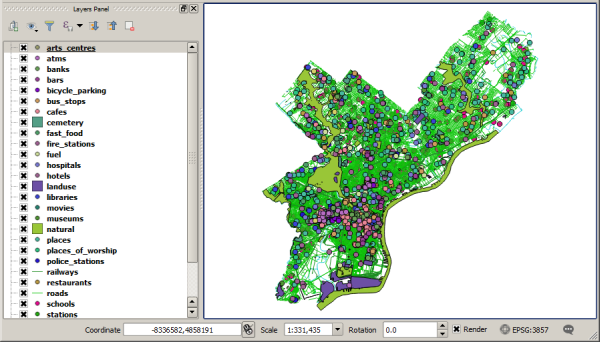 Figure 3.11 QGIS map showing output of the previous operations
Running the OGR utilities in a batch file
If you know that you'll be doing the same series of commands in the future, you can place the commands in a batch file. This is just a basic text file containing a list of commands. On Windows, you just save it with the extension .bat, and then the operating system understands that it should invoke the commands sequentially when you execute the file.
Try the following to see how you could use ogr2ogr in a batch file.
- Once again, delete all files from your clipped and clippedAndProjected folders.
- Create a new text file in any directory and paste in the following text consisting of five command lines (you may need to modify it to match your paths, especially your QGIS installation path which may use a different version name than 3.16.10):
cd /d c:\data\PhiladelphiaBaseLayers
set ogr2ogrPath="c:\program files\QGIS 3.16.10\bin\ogr2ogr.exe"
set GDAL_DATA=C:\program files\QGIS 3.16.10\share\gdal
for %%X in (*.shp) do %ogr2ogrPath% -skipfailures -clipsrc c:\data\PhiladelphiaBaseLayers\clipFeature\city_limits.shp c:\data\PhiladelphiaBaseLayers\clipped\%%X c:\data\PhiladelphiaBaseLayers\%%X
for %%X in (*.shp) do %ogr2ogrPath% -skipfailures -s_srs EPSG:4326 -t_srs EPSG:3857  c:\data\PhiladelphiaBaseLayers\clippedAndProjected\%%X c:\data\PhiladelphiaBaseLayers\clipped\%%X
Notice that these are just the same commands you were running before, with the addition of a few lines at the beginning to change the working directory and set the path of the ogr2ogr utility.
Batch files can use variables, just like you use in other programming languages. You set a variable using the set keyword, then refer to the variable using % signs on either side of its name (for example, %ogr2ogrPath%). Variables created inline with loops are represented in a batch file using %% (for example, %%X), a slight difference from the syntax you use when typing the commands in the command line window.
- Save the file as clipAndProject.bat (make sure there is no .txt in any part of the file name).
- In Windows Explorer, double-click clipAndProject.bat and watch your clipped and projected files appear in their appropriate folders.
Saving the data for future use
You will use this data in future lessons. Therefore, do the following to preserve it in an easy-to-use fashion:
- Create a new folder called Philadelphia, such as c:\data\Philadelphia. This folder will hold all your clipped and projected datasets for future reference.
- Copy all your datasets from the PhiladelphiaBaseLayers\clippedAndProjected folder into the Philadelphia folder.
- Following the techniques earlier in this walkthrough, use QGIS to save a copy of the PhiladelphiaBaseLayers\ClipFeature\city_limits.shp dataset in your new Philadelphia folder. Set the CRS as WGS 84 / Pseudo Mercator. (Remember that this layer was never originally projected, so you need to get a projected copy of it now.)
Walkthrough: Processing raster data with QGIS and GDAL
Now that you've seen QGIS and OGR in action with vector data, you'll get some experience processing raster data. For this exercise, we're going to start with a 30-meter resolution digital elevation model (DEM) for Philadelphia. I obtained this from the USGS National Map Viewer [69]. We'll use a combination of GDAL tools (some of them wrapped in a nice QGIS GUI) to make a nice-looking terrain background for a basemap. This will be accomplished by adding a DEM, a hillshade, and a shaded slope layer together. I have based these instructions on this tutorial by Mapbox [70] that I encourage you to read later if you would like further detail.
Download the Lesson 3 raster data [71]
Extract the data to a folder named PhiladelphiaElevation, such as c:\data\PhiladelphiaElevation. This will contain a single dataset called dem. In the interest of saving time and minimizing the download size, I have already clipped this dataset to the Philadelphia city boundary and projected it to EPSG:3857 for you. If you need to do this kind of thing in the future, you can use the Raster > Projections > Warp command in QGIS, which invokes the gdalwarp command.
- Launch QGIS and use the Add Raster Layer
 button to add dem to your map.
Don't add any vector layers right now. See the note at the end of this walkthrough if you are eventually interested in overlaying shapefiles with your terrain. - Create a hillshade by selecting dem in the table of contents and clicking Raster > Analysis > Hillshade. Save the hillshade as a TIF file named hillshade, and set the parameters as shown in the image below. Then press Run to execute the command.
Note that if you prefer the command line environment, you can make your future hillshades using the gdaldem hillshade command.
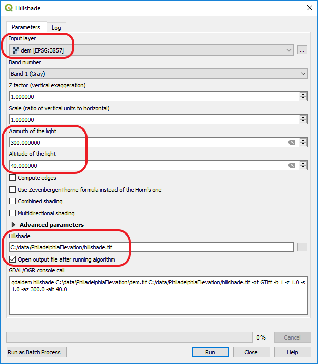 Figure 3.12 Hillshade tool GUI
 - Create a slope surface by highlighting your dem layer in the table of contents and clicking Raster > Analysis > Slope. Save it as a TIF named slope and keep the rest of the defaults. Each pixel in this surface has a value between 0 and 90 indicating the degree of slope in a particular cell.
Now let's shade the slope to provide an extra measure of relief to the hillshade when we combine the two as partially transparent layers. - Create a new text file containing just the following lines, then save it in your PhiladelphiaElevation folder as sloperamp.txt.
0 255 255 255
90 0 0 0
This creates a very simple color ramp that will shade your slope layer in grayscale with values toward 0 being lighter and values toward 90 being darker. When combined with the hillshade, this layer will cause shelfs and cliffs to pop out in your map. - Open your OSGeo4W command line window and use the cd command to change the working directory to your PhiladelphiaElevation folder.
- Run the following command to apply the color ramp to your slope:
gdaldem color-relief slope.tif sloperamp.txt slopeshade.tif
You just ran the gdaldem [72] utility, which does all kinds of things with elevation rasters. In particular, the color-relief command colorizes a raster using the following three parameters (in order): The input raster name, a text file defining the color ramp, and the output file name.
If you add the resulting slopeshade.tif layer to QGIS, you should see this:Now let's switch back to the original DEM and use the same command to put some color into it. Just like in the previous step, you will define a simple color ramp using a text file and use the gdal-dem colorrelief command to apply it to the DEM.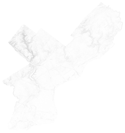 Figure 3.13 Hillshade results
 - Create a new text file and add the following lines (make sure your software doesn't copy it as one big line; there should be line breaks in the same places you see them here). Then save it in your PhiladelphiaElevation folder as demramp.txt.
1 46 154 88
100 251 255 128
1000 224 108 31
2000 200 55 55
3000 215 244 244
Note that the first value in the line is the elevation value of the raster, and the next three values constitute an RGB color definition for cells of that elevation. This particular ramp contains elevations well beyond those seen in Philadelphia, just so you can get an idea of how these ramps are created. I have adjusted the ramp so that lowlands are green and the hilliest areas of Philadelphia are yellow. If we had high mountains in our DEM, brown and other colors would begin to appear. - Run the following command:
gdaldem color-relief dem.tif demramp.txt demcolor.tif
When you add demcolor.tif to QGIS, you should see something like this:This looks good, but the No Data values got classified as green. We need to clip this again. This is a great opportunity for you to practice some raster clipping in QGIS.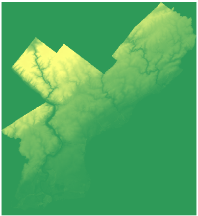 Figure 3.14 DEM sample
 - In QGIS, click Raster > Extraction > Clip raster by mask layer and set up the parameters as below. Make sure you clip demcolor to the city_limits.shp polygon from the previous walkthrough (it should be in PhiladelphiaBaseLayers\clipFeature) and to set the nodata value parameter to 0. Notice that at the bottom of this dialog box, the full gdalwarp syntax (used for clipping) appears in case you ever want to run this action from the command line. This can be a helpful learning tool! Make sure your output file name ends in ".tif" so that the -of GTiff option is added to the gdalwarp command.
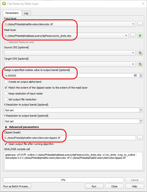 Figure 3.15 Clipper GUI
Now, let's add these together. - Create a new map in QGIS and add the clipped colorized DEM. Then add the hillshade with a 40% opacity. Then add the slopeshade with the 40% opacity. You should get something like below:
Now, play around with the transparencies to suit your liking. You can even re-run the colorization commands to apply different ramps.
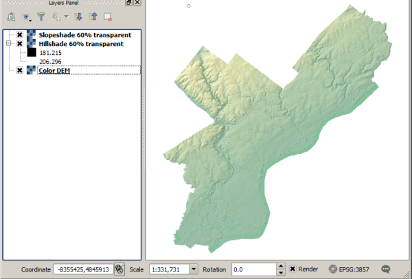 Figure 3.16 Sample map output in QGIS
This type of terrain layer, when overlayed by a few other vector layers, could act as a suitable basemap layer in a web map. In a future lesson, you'll learn how you could create tiles of this type of layer to bring into your web map.
Saving the data for future use
Just like in the previous walkthrough, you will copy your final datasets into your main Philadelphia data folder for future use.
Use Windows Explorer or an equivalent program to copy hillshade.tif, slopeshade.tif, and demcolorclipped.tif into the Philadelphia folder (such as c:\data\Philadelphia) that you created in the previous walkthrough.
Lesson 3 assignment: Prepare term project data and experiment with a GDAL utility
In this week's assignment, you'll get a chance to use some of your newfound QGIS and GDAL skills to prepare your term project data. This assignment has two distinct parts:
- Identify some data of interest (either from your workplace or your own personal interests) that you will use in the term project. The data must include thematic layers and layers suitable for creating a basemap from. So, even if in your final term project you are planning to use available 3rd party basemap options, please obtain some additional data sets that can serve as a background for your thematic data. If necessary, you can create some of the layers yourself.
Download these datasets and get them into the desired format and scope using FOSS tools. Also, project them into the EPSG:3857 projection (one of the tools we'll use later requires it).
Then write 300 - 500 words about your choice of these datasets, also describing the methods and tools you used to process them. Indicate which of the datasets will act as the thematic layer in your eventual web map.
Include relevant screenshots, including an image of your final datasets all shown together in QGIS. Don't worry too much about cartography yet; just show me that you obtained and projected the datasets.
Please note that in your practical workday, you should use whatever tools are easy and available to wrangle your data (including proprietary software); however, in this assignment, I would like you to use FOSS, so you can get some practice with it.
Submit this portion of the assignment to the Lesson 3 (part 1) drop box on Canvas.
- Investigate a GDAL (or OGR) command that you might find useful in your day-to-day work. On the Lesson 3 assignment (part 2) forum on Canvas, post an example of successful syntax that you used with this command, along with "before" and "after" screenshots showing how a dataset was affected by the change. This can be a command that you used in the assignment above, but not one of the commands detailed in the lesson walkthrough. Please make sure to briefly explain the parameters used in your command, unless their meaning is extremely obvious (like input and output file names).
The following pages list the available commands. Although the OGR list looks short, be aware that ogr2ogr has many available parameters and can do a variety of things:
GDAL raster programs [76]
OGR vector programs [77]
Lesson 4: Drawing and querying maps on the server using WMS
The links below provide an outline of the material for this lesson. Be sure to carefully read through the entire lesson before returning to Canvas to submit your assignments.
Note: You can print the entire lesson by clicking on the "Print" link above.
Overview
Up to this point, you have largely worked with data on your local machine using QGIS. In this lesson, you'll take a step into the web world by making some of your map layers available on GeoServer as web services.
This lesson focuses on web services that use the Open Geospatial Consortium (OGC) Web Map Service (WMS) specification. GIS professionals have been using WMS to draw FOSS web maps for years. WMS doesn't use the latest and slickest technology, but it's a functional and widespread specification that's important for you to understand and feel comfortable with.
As part of this lesson, you'll practice serving some of your term project data as a WMS; however, you are not required to use the layer in your term project if you decide there is a more appropriate format. As you'll see in the next few lessons, there are various other ways to draw layers in a web map.
Objectives
- Identify the pros and cons to using a dynamically drawn web map service (as opposed to a tiled service).
- Recognize the role of OGC in defining open geospatial web service specifications.
- List the basic functions of a WMS and describe how and why each would be invoked.
- Expose GIS datasets as a WMS using GeoServer.
- Use SLDs to define layer styling in a WMS. Create the SLDs using code and using the GUI environment of QGIS.
- Identify and critique a WMS used in a public-facing website.
Checklist
- Read the Lesson 4 materials on this page.
- Complete the two walkthroughs.
- Complete the Lesson 4 assignment.
Dynamically drawn map services
There are various ways to get a map to show up in someone's web browser. One way is for the server to send predrawn map images (or image tiles) to the browser, another way is for the server to send a bunch of text-based geographic coordinates and attributes that the browser draws, and a third way is to draw the map on the server at the time of request and send the browser the completed map image. This third way is what we'll discuss in this lesson. It's sometimes called a dynamic map service because, being drawn on the fly, it reflects the most recent picture of the data. Contrast this with the image tile approach, which represents a static picture of the data taken at one point in time (when all the tiles were generated).
Advantages of dynamically drawn map services
Because dynamically drawn map services retrieve the data and draw it at the time of request, they are useful for gaining a situational awareness of the most recent state of the data. They may be the only reasonable way to depict many features that are changing at the same time (such as the positions of each vehicle in a large fleet). Dynamically drawn maps may also be the best solution at large scales where tiled maps become too cumbersome to generate, store, or maintain.
Maps dynamically drawn through WMS allow you to apply a wide range of symbols and styles using a concept called Styled Layer Descriptors (SLDs), which is described later in this lesson. If you enjoy using the QGIS authoring environment for your maps, you can export an SLD and import it into GeoServer, thereby allowing web users to apply the same styling that you configured on the desktop. Map layers drawn by the web browser may not be able to use symbols as complex as ones drawn by the server.
Disadvantages of dynamically drawn map services
Waiting for the server to draw the map can be a slow, painful experience, especially if there are many layers to render. A wait time of 2 - 3 seconds that may be considered acceptable on the desktop may not be tolerated by edgy web map users who are neither knowledgeable nor sympathetic to the type of back end technology being used. People now expect every map to perform as fast as Google Maps and, without using tiles, this can be difficult to achieve.
Dynamically drawn services are also much more susceptible to overload than tiled services if you have many users deciding they want to see the map at the same time. This presents a paradox: you want your map to be useful, but the more exposure it gets, the slower it will run if the server technology is not scalable.
If you know you have a limited audience for your application (such as a small municipality, or a team of scientists), you may safely decide that the performance of your dynamically drawn map service is "good enough." This can spare you the work of generating and maintaining a tiled service.
Server software for dynamically drawn maps
In this course, you'll use GeoServer for drawing dynamic map services through WMS. Other FOSS software that can do this includes:
- Map Server [20] - Sometimes called the "Minnesota Map Server," this was developed at the University of Minnesota in the 1990s.
- QGIS Server [21] - An extension for QGIS that allows you to publish your QGIS map directly through WMS.
- Deegree [78] - Java-based FOSS for GIS web services, born out of Germany in the early 2000s.
- Others? - Because WMS is an open specification, any developer with enough skill and gumption can develop server software that supports it. Have you used any other FOSS software for creating WMS? Let us know about it in the course forums.
Proprietary GIS software such as Esri ArcGIS Server also supports WMS and other OGC specifications. Although Esri has their own format for map services, many of their clients have interoperability requirements mandating that their web services be available through WMS. Hence, when you publish a map service in ArcGIS Server, you see a checkbox that can allow the service to speak through WMS specifications.
Open specifications for web map services
In the previous lesson, you learned about some open formats for data stored on your machine as files and databases. Now, let's examine some of the open specifications for web services that draw maps.
What is a specification document?
Recall from Lesson 1 that a web service receives a user request and sends back a response. In order for web services to work across platforms, the syntax for the requests and responses needs to be consistent and openly described in what is called a "specification" document. When software developers create a server or a client that supports the web service, they treat the specification document as their Bible; it is a contract that must be closely honored in order for web services to correctly function.
To get a feel for what a specification looks like, take a minute to browse the Open Geospatial Consortium (OGC) WMS specification [79] (especially Section 7). Don't worry too much about what this all means. We'll dive into some of that later in the lesson. Just notice that there are clearly defined methods and parameters that you and the server must use if you want to communicate with the service.
Because specifications must describe every method and parameter of the web service, they can appear to be long and complicated documents. Fortunately, you rarely have to use the specification directly because you will work with relatively user-friendly servers and clients are designed to abstract away the complexity of working with web services. For example, later in this lesson, you'll use GeoServer to create a WMS and QGIS to display the WMS on a map. You don't have to refer to the WMS specification in order to do this because these programs take care of formulating the request and working with the response. You can be certain, however, that the developers of GeoServer and QGIS had to examine the WMS specification in great detail when writing their source code.
OGC W*S specifications
The OGC is an industry consortium that develops open specifications for spatial data and web services. The OGC is comprised of representatives from private companies, government organizations, NGOs, and universities.
OGC has produced a series of specifications for GIS web services named in the format Web _____ Service (sometimes abbreviated as W*S). For example:
- Web Map Services (WMS) return a rasterized image of a map drawn by the server. This doesn't allow much complex analysis, but it is so useful for visualization that WMS has become the most widely implemented and supported of the W*S services.
The basic WMS draws the map on the fly, but additions to the WMS specification provide syntax for requesting predrawn image tiles from the server. To get started, we'll just work with the dynamically drawn WMS. - Web Feature Services (WFS) return vector geometries and attributes, allowing for spatial analysis and editing. The vector features are communicated in XML using Geography Markup Language (GML), itself an open specification defined by the OGC for transferring vector feature data.
- Web Coverage Services (WCS) return blocks of data called coverages (not to be confused with the old vector Arc/INFO coverages) that are commonly used for raster display and analysis.
- Web Processing Services (WPS) allow a user to invoke geoprocessing operations on the server.
Virtually all FOSS GIS servers and some proprietary ones have engineered their web services to communicate through OGC specifications. Additionally, many client APIs for developing web maps, such as OpenLayers and Leaflet, support WMS as web map layers. Desktop GIS programs like QGIS support the use of WMS as layers. In fact, the buttons  allow you to add (from left to right) WMS, WCS, and WFS web services as layers in QGIS.
The GeoServices REST Specification
In 2010, the proprietary GIS software company Esri released an open document called the GeoServices REST Specification (now the GeoServices API [80]) describing the request and response patterns used by default for its ArcGIS Server web services. (Although I mentioned that you can enable OGC communication on an ArcGIS Server service, this option is not the default.)
The GeoServices REST Specification uses a RESTful pattern of communication with the web services. Whereas the OGC services offer a simple list of methods that typically return XML (when they're not returning an image), REST exposes information in a navigable hierarchy of URLs that can return focused packets of HTML, JSON, images, or other data types. For example, using REST and the GeoServices REST specification, you can invoke http://<server>/MapServer/layers/ to get a list of layers in a map service and
Although ArcGIS Server had already been using this pattern of communication for several years, Esri eventually placed the specification online as an open document so that developers would feel encouraged (or at least legally allowed) to implement clients and servers supporting this pattern.
Some controversy around the specification erupted in 2013 when a slightly modified version of the document (with the Esri references scrubbed out) was submitted to a vote for adoption as an OGC specification. Proponents, including Esri, argued that the OGC lacked a nimble, RESTful alternative to the W*S specifications (this lesson previously linked to a 2013 Esri User Conference Q & A item elaborating this argument, but this document has since been taken offline). Opponents expressed concern [81] about functional overlap with existing service types, and claimed that OGC adoption of the specification would give Esri an unfair advantage in competing for contracts. The uproar was significant enough to get the specification pulled from the voting process.
Although the GeoServices REST Specification is not an OGC specification, I am mentioning it in this lesson as an example of a specification that was voluntarily made open by a proprietary software vendor for the purposes of encouraging interoperability and the proliferation of the vendor's platform. It is likely that you will encounter this specification at some point in your career if you do any development with web services that somebody has hosted on ArcGIS Server.
Basics of the WMS specification
The Open Geospatial Consortium (OGC) Web Map Service (WMS) specification provides a pattern for serving maps through web services. The WMS receives a request detailing the bounding box (or extent) of the map, the layers to include, the projection to use, and other parameters. It returns a rasterized map image in a common format such as JPG, GIF, or PNG. It does not return any actual GIS data, although an optional part of the specification describes how a user can query any pixel of the service to retrieve attribute information.
WMS has been around since the year 2000 and was supported by some of the earliest FOSS GIS servers. It is still widely supported today in FOSS and proprietary GIS software. Although it has been sometimes criticized as clunky, WMS has enabled a greater degree of interoperability in the world of online mapping.
Consider WMS as an option if you do need a high level of interoperability, and you don't require lightning fast performance or the ability to handle dozens of concurrent users. If you need greater performance and scalability, you should consider tiled maps, including the OGC-endorsed WMTS (Web Map Tile Service) specification. Tiled map services are described in the next lesson.
Requesting a map from a WMS using the GetMap operation
The best way to get familiar with WMSs is to look at a real one. Therefore, make a close examination of the following URL and then open the link in a web browser:
This request uses the WMS's GetMap operation to retrieve a map with a land cover classification based on imagery and LiDAR data for the State College area. If you are familiar with the campus, you may recognize some buildings and roads in the image. This WMS is provided by the PASDA web portal [83].
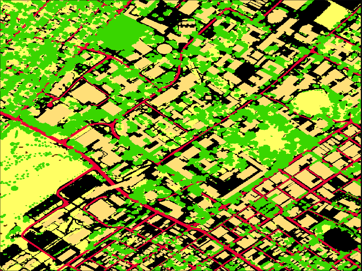
Although a WMS can perform several types of operations, GetMap is the most common. It's the one that sends you back a map image.
The root piece of a WMS URL (https://imagery.pasda.psu.edu/arcgis/services/pasda/UrbanTreeCanopy_Landcover/MapServer/WmsServer? [84]) can be formed in various ways (often it will end in 'wms?' rather than 'WmsServer?'), but the parameters following the ? must be formatted according to the WMS specification. Let's examine the parameters used in the above URL.
| Parameter | Example value | Notes |
|---|---|---|
| SERVICE | WMS | Indicates that a WMS is being called. |
| VERSION | 1.1.1 | The version of the WMS specification that this WMS can be expected to comply with |
| REQUEST | GetMap | This is the operation being requested from the WMS. The GetMap method is the most common operation called on a WMS and is the one that actually returns a map image. The GetCapabilities method is another common operation that returns you some XML metadata describing what the WMS can do. |
| LAYERS | 10 | A comma-delimited list of layers that the WMS should include when it draws the map. Some WMSs (like this one) are treated as collections of separate layers that are not intended to be drawn together. Other WMSs have the layers designed to be overlayed or drawn in groups. In this WMS, the layers have numbers as names but these can also be real names like "landcover_2006_statecollege". |
| STYLES | In this parameter, you can define your own styles to apply to the WMS when it is drawn. We did not submit this parameter, therefore we get the default styling defined on the server. | |
| SRS | EPSG:4326 | The coordinate system that the WMS will use when it draws the map. Here it is specified using an EPSG code (which you saw in previous lessons). Clients can request the WMS to be drawn in WGS 84 (EPSG:4326) or any coordinate system that the WMS publisher has explicitly enabled on the WMS. If you're not sure what coordinate systems the WMS publisher has enabled, then you could use the GetCapabilities method to find out before requesting a map image. |
| BBOX | -77.87304,40.78975,-77.85828, 40.80228 | The rectangular extent of the map to be returned by the WMS. This is given by specifying the coordinates of the lower left corner and the upper right corner in a comma delimited fashion. |
| FORMAT | image/png | The image format that should be returned by the WMS. In this case, the server will return a PNG. Your choice can affect the performance of your service. For remotely sensed imagery, a format like image/jpeg might result in less data being transferred between the server and the client (and therefore a faster draw time). |
| WIDTH | 1200 | The width, in pixels, of the image to be returned. |
| HEIGHT | 900 | The height, in pixels, of the image to be returned. |
When you request a map from a WMS, there are some required parameters that you must supply and some optional parameters that you may decide to supply if the WMS publisher has implemented them. All the parameters in the above table are required. Optional parameters can display things like time and elevation dimensions. Table 8 in Section 7.3.2 of the Version 1.3.0 WMS Specification [79] shows all parameters for the GetMap request and whether they are required or optional. If you have questions about how to format the parameters, you can always refer to the specification; however, most GIS software gives you user-friendly interfaces for interacting with WMSs so that you don't have to formulate the URLs yourself.
Other WMS operations
Besides the GetMap request, WMS supports one other required operation (GetCapabilities) and an optional operation (GetFeatureInfo).
GetCapabilities
The GetCapabilities request returns metadata about the service, which you can use as a guide when making other types of requests. Here's what a GetCapabilities request would look like for ourland cover WMS:
Take a look through the XML response returned in your web browser when you hit the above URL
Notice that you can see information about each layer in the WMS, which is helpful when you are making a GetMap request and you want to know the appropriate names to specify for the LAYERS parameter.
<Layer queryable="1">
   <Name>10</Name>
   <Title>
     <![CDATA[ LandCover_UTC_2006_StateCollege ]]>
   </Title>
   <Abstract>
     <![CDATA[ ]]>
  </Abstract>
   ...
</Layer>
You can also see a list of the spatial reference systems that the service publisher has decided to support for the layer.
<CRS>CRS:84</CRS>
<CRS>EPSG:4326</CRS>
<CRS>CRS:4269</CRS>
GetFeatureInfo
GetFeatureInfo is an optional method that the service publisher can enable, allowing users to query the attribute data of a WMS layer at a specific location. This makes it possible to add interactive elements such as informational popups without enlisting the help of a second web service.
When you make a GetFeatureInfo request, you supply many of the same parameters as the GetMap request, with the addition of the screen coordinates of the pixel you want to query.
The land cover example says that the layer 9 is queryable, so try the following query URL to query for the feature at coordinates x=600 and y=300 within the map image with width=1200 and height=900:
The returned plain text response, in this case, will tell you that there that the pixel value for these coordinates is 5 which according to the description at PASDA [83] means 'building':
@10
PixelValue;OBJECTID;COUNT;
5;5;1378041;
GetFeatureInfo is somewhat of a wildcard, because the WMS specification does not mandate any particular structure or format for the returned information. If you don't know who published the service, you must make a request and examine the response in order to understand how to work with the returned information. The GetCapabilities response can show you the supported INFO_FORMATs you can request:
<GetFeatureInfo>
   <Format>application/vnd.esri.wms_raw_xml</Format>
   <Format>application/vnd.esri.wms_featureinfo_xml</Format>
   <Format>application/vnd.ogc.wms_xml</Format>
   <Format>text/xml</Format>
   <Format>text/html</Format>
   <Format>text/plain</Format>
   ...
</GetFeatureInfo>
Applying styles and symbols to a WMS
The OGC allows some flexibility to adjust the map symbols used in WMS layers. This is accomplished by referencing a chunk of XML called a Styled Layer Descriptor (SLD). An SLD describes all the symbol sizes, colors, and markers that should be applied within the WMS. SLDs are complex enough that they have their own OGC specification documents [87] defining how they are supposed to operate.
SLDs can be designed by either the service publisher or the client. To formulate a really useful SLD, you have to know a little bit about the layers in the WMS. You can get this by calling the optional DescribeLayer operation on the WMS.
Once you've created the XML for your SLD, you can apply it in one of several ways. The most common way is to put the SLD in its own file on a web server somewhere, and reference the URL of that file when you make a GetMap request. There is an optional SLD parameter in the GetMap request that you can use for this very purpose. Another way is to use the optional SLD_BODY parameter of the GetMap request and just provide the relevant chunk of XML directly in the URL of the request. This obviously can create long and unwieldy URLs, and requires a lot of special character encoding or escaping.
The XML used with SLDs can get verbose and tends to contain many nested levels. Because of this, it's unlikely that you'll sit down to compose an SLD from scratch. Instead, you'll probably start with a sample and adjust it to meet your needs. Alternatively, you can use the GUI environment from QGIS to style a layer and then save it out as an SLD.
Both approaches (starting an SLD from an existing sample and exporting an SLD from QGIS) are covered in the lesson walkthrough.
SLDs and GeoServer
GeoServer maintains your data information and your style information completely separate. In the Layers page you define what datasets you want to serve, and in the Styles page you define all the SLDs you want available. The Publishing tab of the Edit Layer page is the (somewhat obscure) place where you connect the dots and define which style will be applied to your layer.
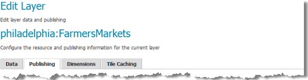
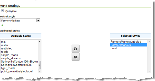
In the above graphic, the GeoServer administrator has examined the pool of all styles added to GeoServer (left) and selected three of those (right) to be available for use with the FarmersMarkets layer. The WMS will advertise these three styles for the layer and will use the one called FarmersMarkets if the user does not specify a different style in the STYLES parameter of the GetMap request.
The examples below are not functional, but they show you the URL structure for requesting different styles.
GetMap request that uses the default style ("FarmersMarkets"):
http://localhost:8080/geoserver/philadelphia/wms?service=WMS&version=1.1.0&request=GetMap&layers=philadelphia:FarmersMarkets&styles=&bbox=-8377237.031452011,4854963.883290707,-8357515.816574659,4877579.355521561&width=446&height=512&srs=EPSG:3857&format=image%2Fpng
GetMap request that overrides the default style and uses the style named "point" instead:
http://localhost:8080/geoserver/philadelphia/wms?service=WMS&version=1.1.0&request=GetMap&layers=philadelphia:FarmersMarkets&styles=point&bbox=-8377237.031452011,4854963.883290707,-8357515.816574659,4877579.355521561&width=446&height=512&srs=EPSG:3857&format=image%2Fpng
Notice that the latter URL includes styles=point, indicating that GeoServer should use the SLD named "point" to draw the layer. Alternatively, the user could have specified styles=FarmersMarketsLabeled.
Required reading
Before you move on, please read the following pages of GeoServer documentation. This contains general information about SLDs, technical notes about how SLDs are applied in GeoServer, and a set of example SLDs that you can use to get started when it comes time to make your own. You'll get some practice with this technology during the walkthrough, but it is well worth your time to become familiar with this particular section of the documentation. In fact, it might be wise to read it both before and after you complete the walkthrough in order for you to confirm your learning and absorb the maximum amount of information.
- Introduction to SLD [88]
- Working with SLD [89]
- SLD Cookbook [90]
- Three or four examples of your choosing from the SLD Cookbook
Walkthrough: Serving and styling a WMS with GeoServer
In this walkthrough, you'll get some practice serving some geographic data as a WMS using GeoServer. The exercise will progress from simple to complex in the following manner:
- Serving a single layer as a WMS using the default styling
- Applying a style to the WMS using an SLD
- Viewing the WMS in QGIS
The next walkthrough will go into more depth with SLDs and group layers.
As you complete these walkthroughs, think of some of your own data you'd like to serve as a WMS in fulfillment of the Lesson 4 assignment. You won't be required to use this WMS in your term project, but you can if you choose.
Serving a single layer as a WMS using the default styling
Let's start out by serving a single layer as a WMS. We'll stick with Philadelphia in this lesson so that we can eventually pull in some of the base layers that we clipped and projected previously. The first layer we'll work with is a polygon dataset of Philadelphia neighborhoods that I derived from a Zillow.com [91] shapefile.
- Download Neighborhoods.zip [92] and extract the contents into your Philadelphia data folder so that the files can be found at a path like c:\data\Philadelphia\Neighborhoods.shp. This data is already projected into EPSG:3857 and it doesn't need to be clipped for this exercise.
- Start GeoServer by running the startup.bat script from the bin subfolder.
- Start the GeoServer Web Admin Page by opening the URL localhost:8080/geoserver/web in your browser and log in with your administrator account (the username is probably "admin" with password "geoserver"). Refer to Lesson 2 if you need a refresher.
The first thing you will do is create a workspace and a store. A workspace is a place where you can organize datasets for a project. A store is an actual folder or database. A workspace can contain multiple stores. Our scenario is pretty simple because you'll have one workspace and one store; however, if your data were spread out among many folders or databases, you would need to create more stores. - In the left-hand menu, click Workspaces. You'll see some sample workspaces.
- Click Add New Workspace.
- In the Name field, type geog585.
- In the Namespace URI field type http://localhost:8080/geoserver/geog585 [93] and then click Save. The Namespace URI doesn't have to be a real URL; it only needs to be a unique identifier. The GeoServer documentation suggests using a URL- like structure with the name of the workspace appended to it.
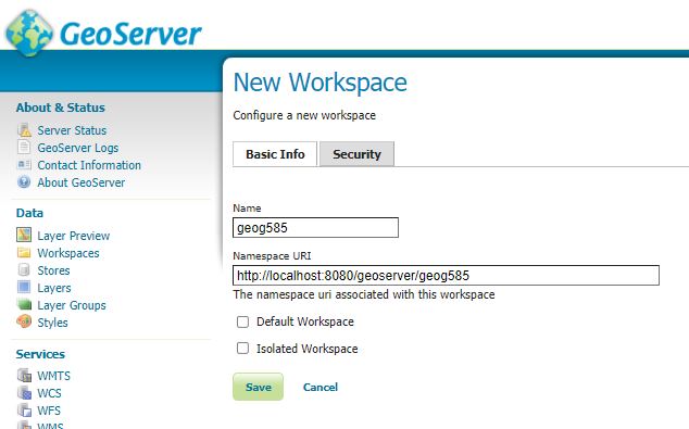 Figure 4.4 Configuring a new workspace in GeoServer
 - In the left-hand menu, click Stores and click Add New Store.
Examine the types of stores you can add. Notice that if you are going to use raster data with GeoServer, you need to add it as a separate store from your vector data. In this exercise, we'll just be working with the folder of vector shapefiles of Philadelphia that you've collected during this course. This should be located at a path similar to c:\data\Philadelphia. - Click Directory of spatial files (shapefiles).
- Complete the dialog box as in the graphic below, designating philadelphia as the name of the data source and browsing to your Philadelphia data folder where prompted to specify the directory of shapefiles.
When you are finished, click Save. Note that you can create this store even though there are raster files in it. If you wanted to use the rasters, though, you would have to specify a separate store in GeoServer.
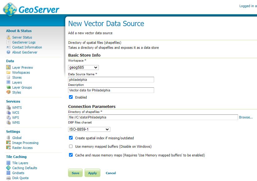 Figure 4.5 Defining a new vector data source in GeoServer
Now you will go one level further and specify the actual shapefile that you want to expose as a layer. - Click Layers > Add a New Layer. You'll be prompted to choose the store that will supply the layer.
- Choose to add the layer from geog585:philadelphia. You should see a list of layers from your Philadelphia folder.
- Find the Neighborhoods layer and click its Publish link.
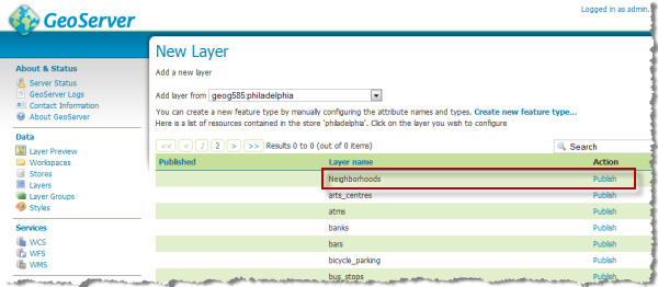 Figure 4.6 Adding the newly defined layer in GeoServer
 - At this point, you'll see a lot of options for publishing the layer. Leave the defaults near the top of the page, but scroll down until you come to the Coordinate Reference Systems section of the page and set it up as in the image below. Note that instead of manually filling in the bounding box coordinates, you just need to click the links Compute from data and Compute from native bounds in order to fill in the bounding boxes. Prior to doing this, you need to make sure you declare your SRS as EPSG:3857 (you must browse to this, not type it in) and that you set your SRS handling to Force declared. This allows you to serve data that is using the common web-based Mercator projection.
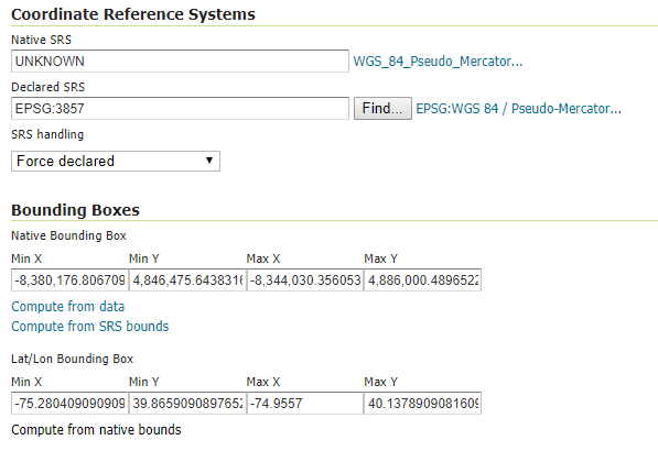 Figure 4.7 Setting the Coordinate Reference System (CRS) in GeoServer
Various programs have different ways of interpreting EPSG:3857, and some of them don't always match. I have found that if I do not set Force declared, my WMS is offset from other EPSG:3857 data by about 20 km when I try to display it all in QGIS. - Scroll down to the bottom of the page and click Save.
You should now see your layer appearing in the layer list. Let's take a look at it in a preview window. - In the left-hand menu, click Layer Preview. Then find your layer in the list.
- Choose to preview your layer as a WMS in the OpenLayers 3 example window.
You should see a basic map like this:
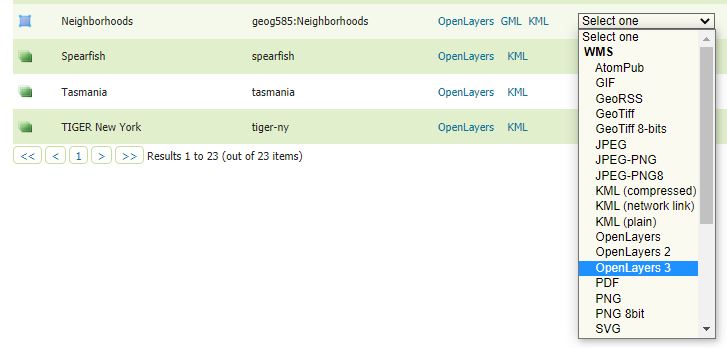 Figure 4.8 Setting up the preview of the new layer in GeoServerNotice the URL parameters above are the standard ones that you've learned about for WMS requests.
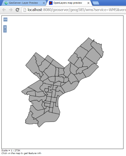 Figure 4.9 Output of the preview in GeoServer
Styling the WMS using SLDs
The above WMS indeed contains the Philadelphia neighborhoods, but there are no labels and we didn't get to choose the color scheme. In this part of the walkthrough, you'll use an SLD to apply a blue outline and labels with no fill. This will allow the neighborhoods WMS to act as a thematic layer that you can place on top of other base layers.
To work with SLDs in GeoServer, you first add the SLD under the Styles list. Then you can go back into the layer properties and apply the style. Decoupling the styles and the layers in this fashion allows you to reuse a particular style on multiple layers.
The first thing we'll do is prepare the SLD, starting with an existing sample and then modifying it to meet our needs.
- Open the SLD Cookbook to the Polygon with styled label [94] example. This comes pretty close to what we want, so we're going to start with it.
- Click View and download the full "Polygon with styled label" SLD. You will see the XML of the SLD example.
- Use your browser's save option to save the page contents with a file extension of .sld. For example: polygonwithstyledlabel.sld
Do not copy and paste the XML out of the browser window, or you may fail to get the full XML headers and GeoServer won't like it. You must save the page as a .sld file. - Open the .sld file in a text editor like Notepad and take a close look at the PolygonSymbolizer and TextSymbolizer options. You should see something like this:
<?xml version="1.0" encoding="ISO-8859-1"?>
		<StyledLayerDescriptor version="1.0.0"
		    xsi:schemaLocation="http://www.opengis.net/sld StyledLayerDescriptor.xsd"
		    xmlns="http://www.opengis.net/sld"
		    xmlns:ogc="http://www.opengis.net/ogc"
		    xmlns:xlink="http://www.w3.org/1999/xlink"
		    xmlns:xsi="http://www.w3.org/2001/XMLSchema-instance">
		  <NamedLayer>
		    <Name>Polygon with styled label</Name>
		    <UserStyle>
		      <Title>SLD Cook Book: Polygon with styled label</Title>
		      <FeatureTypeStyle>
		        <Rule>
		          <PolygonSymbolizer>
		            <Fill>
		              <CssParameter name="fill">#40FF40</CssParameter>
		            </Fill>
		            <Stroke>
		              <CssParameter name="stroke">#FFFFFF</CssParameter>
		              <CssParameter name="stroke-width">2</CssParameter>
		            </Stroke>
		          </PolygonSymbolizer>
		          <TextSymbolizer>
		            <Label>
		              <ogc:PropertyName>name</ogc:PropertyName>
		            </Label>
		            <Font>
		              <CssParameter name="font-family">Arial</CssParameter>
		              <CssParameter name="font-size">11</CssParameter>
		              <CssParameter name="font-style">normal</CssParameter>
		              <CssParameter name="font-weight">bold</CssParameter>
		            </Font>
		            <LabelPlacement>
		              <PointPlacement>
		                <AnchorPoint>
		                  <AnchorPointX>0.5</AnchorPointX>
		                  <AnchorPointY>0.5</AnchorPointY>
		                </AnchorPoint>
		              </PointPlacement>
		            </LabelPlacement>
		            <Fill>
		              <CssParameter name="fill">#000000</CssParameter>
		            </Fill>
		            <VendorOption name="autoWrap">60</VendorOption>
		            <VendorOption name="maxDisplacement">150</VendorOption>
		          </TextSymbolizer>
		        </Rule>
		      </FeatureTypeStyle>
		    </UserStyle>
		  </NamedLayer>
		</StyledLayerDescriptor>
Notice the places where the stroke and fill colors are specified, as well as the text weight and font. Also notice the tags marked VendorOption, which are not part of all SLDs but are supported by GeoServer as a special means of finding suitable label locations (maxDisplacement) and forcing the labels to wrap after reaching a certain length (autoWrap). See this GeoServer documentation [95] for details.
Let's edit the SLD to make a blue outline with a hollow fill, as well as blue labels. It is also critical that we change the name of the field that is supplying the label text (specified in the tag ogc:PropertyName). By default, in this example, the field is "name" but in our neighborhoods shapefile it is "NAME". The case sensitivity matters. - Replace your original SLD text with the following, either carefully editing line by line or completely copying and pasting the text below. Make sure you understand which lines changed and why.
<?xml version="1.0" encoding="ISO-8859-1"?>
		<StyledLayerDescriptor version="1.0.0"
		   xsi:schemaLocation="http://www.opengis.net/sld StyledLayerDescriptor.xsd"
		   xmlns="http://www.opengis.net/sld"
		   xmlns:ogc="http://www.opengis.net/ogc"
		   xmlns:xlink="http://www.w3.org/1999/xlink"
		   xmlns:xsi="http://www.w3.org/2001/XMLSchema-instance">
		  <NamedLayer>
		   <Name>Polygon with styled label</Name>
		   <UserStyle>
		    <Title>SLD Cook Book: Polygon with styled label</Title>
		    <FeatureTypeStyle>
		     <Rule>
		<PolygonSymbolizer>
		       <Stroke>
		        <CssParameter name="stroke">#133E73</CssParameter>
		        <CssParameter name="stroke-width">2</CssParameter>
		       </Stroke>
		      </PolygonSymbolizer>
		      <TextSymbolizer>
		       <Label>
		        <ogc:PropertyName>NAME</ogc:PropertyName>
		       </Label>
		       <Font>
		        <CssParameter name="font-family">Arial</CssParameter>
		        <CssParameter name="font-size">11</CssParameter>
		        <CssParameter name="font-style">normal</CssParameter>
		        <CssParameter name="font-weight">bold</CssParameter>
		       </Font>
		       <LabelPlacement>
		        <PointPlacement>
		         <AnchorPoint>
		          <AnchorPointX>0.5</AnchorPointX>
		          <AnchorPointY>0.5</AnchorPointY>
		         </AnchorPoint>
		        </PointPlacement>
		       </LabelPlacement>
		       <Fill>
		        <CssParameter name="fill">#133E73</CssParameter>
		       </Fill>
		       <VendorOption name="autoWrap">60</VendorOption>
		       <VendorOption name="maxDisplacement">150</VendorOption>
		      </TextSymbolizer>
		     </Rule>
		    </FeatureTypeStyle>
		   </UserStyle>
		  </NamedLayer>
		</StyledLayerDescriptor>
- Save this text file (making sure you keep the extension as .sld) and open the GeoServer Web Admin Page.
- In the GeoServer Web Admin Page, click the Styles link in the left-hand menu.
Notice there are some styles pre-loaded for you. You can also define your own, which we'll do. - Click Add a new style.
- Before giving the style a name and a workspace, scroll down below the code window and click the Choose File button under "Upload a style file".
- Browse to the .sld file you just created, then click the Upload link. You should see the code load into the window.
- Now name your SLD PolygonWithStyledLabel and place it in the geog585 workspace.
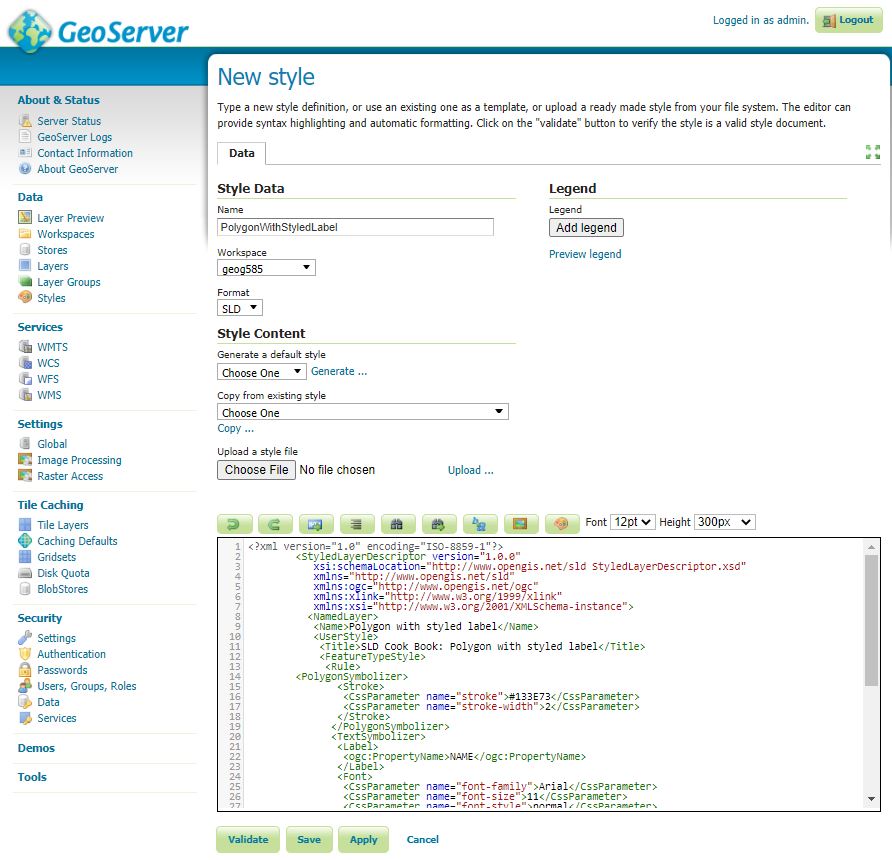 Figure 4.10 Defining / applying the new SLD in GeoServer
 - Scroll to the bottom of the page and click Save to create your style. Before doing this, you can click Validate to make sure your XML is acceptable to GeoServer.
You can come back to this page any time to make edits to your SLD. Any services using the SLD will be immediately updated.
Now let's apply this SLD to the neighborhoods layer. - In the left-hand menu, click Layers.
- Find your neighborhoods layer in the table and click the actual link that says Neighborhoods. This should take you to the Edit Layer page.
- Click the Publishing tab and scroll down to WMS Settings.
- In the Available Styles list, find your geog585:PolygonWithStyledLabel style and click the arrow button to move it over. Then set the Default style to PolygonWithStyledLabel.
Notice that a layer can advertise various styles, but you can choose which one gets applied by default. The alternate style in this case would be the basic gray polygon.
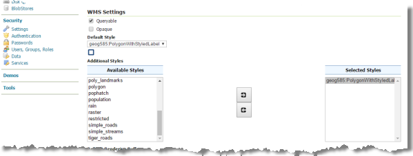 Figure 4.11
 - Click Save to preserve your changes.
- Use the Layer Preview link to preview your neighborhoods in the OpenLayers viewer as you did earlier in this walkthrough.
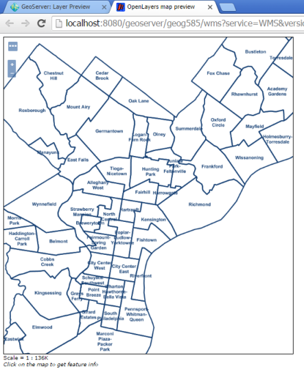 Figure 4.12 Preview of the data styled with our new SLD
This is still not perfect (notice the many labels overlapping features), but it is progress, and it has opened the door to editing the style through other XML options defined in the SLD and GeoServer documentation.
In general, labeling is a tricky subject with web maps. Labeling is computationally intensive and relies on complex rules that can slow down the map drawing. The labeling rules available with GeoServer and WMS are relatively simple compared to the logic used by a desktop program like QGIS or ArcMap. Because of these issues, web map authors sometimes rely on alternative mechanisms such as interactive popups or text that changes dynamically depending on where you point or click the mouse (or tap the display). Fetching this information on demand is faster than waiting for thousands of labels to be placed and eliminates the reliance on complex labeling algorithms.
Viewing the WMS in QGIS
There are lots of clients you can use to view a WMS. You already saw how your WMS could be previewed with OpenLayers. Now let's take a few minutes to see how QGIS works with WMS layers. This is important if you want to bring web services into your desktop maps as backgrounds or thematic layers.
- Launch QGIS, start a new project, and click the Add WMS/WMTS Layer button.

- In the Layers tab, click the New button. Here you will put the properties of your GeoServer workspace. All the layers in your workspace are exposed through the same root WMS URL.
- Enter the name as Geog585 Layers and the URL as http://localhost:8080/geoserver/geog585/wms [96] as shown below. Notice that the geog585 in the URL is the name of the workspace you created in GeoServer.
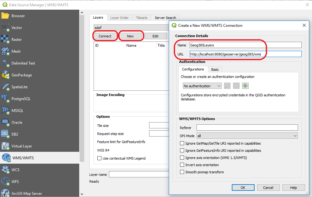 Figure 4.13 WMS connection dialog
 - Click OK and then click Connect.
- Select the Neighborhoods layer and click Change. A WMS by default can display itself in EPSG:4326 (WGS 84 geographic coordinates) or any other coordinate systems that the server administrator would like to support. Your WMS supports EPSG:3857 and that's what you'd like to request from the server here in your maps.
- Set the coordinate reference system to EPSG:3857 and click OK.
- Make sure your dialog box looks like the one below. Click Add to add the layer, and then click Close to close the dialog box.
You should see the layer added to the display like this:
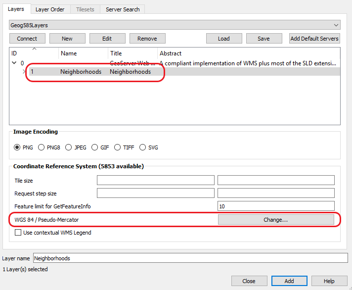 Figure 4.14 QGIS Add WMS layer dialogThis is a good time to use the OpenLayers plugin that you may already have installed in Lesson 3. At the end, I'll also explain how you can do the same thing without the OpenLayers plugin.
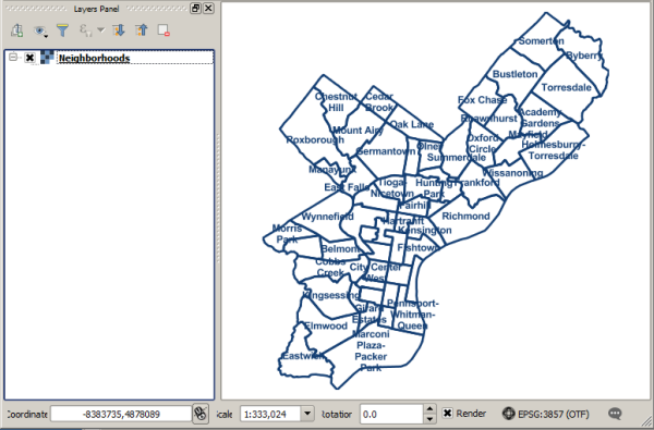 Figure 4.15 QGIS layer list example
First of all, if you did not install the OpenLayers plugin, please have a look at section "Processing spatial data with FOSS" [97] again. Let's put a simple basemap beneath this to give it some geographic context. - In QGIS, click Web > OpenLayers plugin > OSM/Stamen > Stamen Watercolor/OSM.
- Rearrange your layers so that the OSM streets are on the bottom.
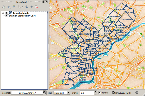 Figure 4.16 QGIS sample output showing our WMS layer and a styled OpenStreetMap layer
If you don't have the OpenLayers plugin installed, you can still add the Stamen Watercolor map. You do this by pointing QGIS at the basemap image tiles on the Stamen servers. First, make sure your Browser panel is open. If necessary, click View > Panels > Browser. In the list of layer types in the Browser panel, find the XYZ Tiles item, right-click it, and choose New Connection. Enter the Name as "Stamen watercolor" and enter the URL as http://c.tile.stamen.com/watercolor/{z}/{x}/{y}.jpg . This is the generic URL structure for the Stamen Watercolor tiled map images (more on this in Lesson 5), where x is the column, y is the row, and z is the zoom level of the tile to fetch at any given map extent. Click OK, and then drag and drop the resulting Stamen Watercolor layer down into your map layer list in the Layers panel. See this post [98] for tips on adding all kinds of other basemap layers to QGIS 3 in the same fashion.
Congratulations! You have just made a (somewhat strange) "mashup" that brings in web services from two different servers. In future lessons, you'll learn how to do this in a more practical fashion in a web application.
QGIS not only displays WMS layers; it can also help you create SLDs. In the next walkthrough, you'll make some SLDs using QGIS and learn how to group WMS layers together using GeoServer.
Walkthrough: Advanced styling and group layers with WMS
You've learned how to serve and style a single layer as a WMS using GeoServer and some basic SLD examples. Now, you'll go a bit further and use QGIS to set up your styles for you. You'll also see how you can group multiple WMS layers using GeoServer.
Some of the steps require you to apply the skills you learned in the previous walkthrough. You may need to pause and review in order to complete these steps.
Creating SLDs with QGIS
QGIS allows you to save out your current layer symbology as an SLD. You then apply the SLD in GeoServer using the same procedure you learned in the previous walkthrough. Styling layers in QGIS is a lot easier than writing XML. However, be aware that some features, such as labels, are not saved in the SLD. Also, the style may look slightly different when you apply it in GeoServer. Be prepared to use some trial and error to get things exactly right.
Let's style a couple of the other Philadelphia base layers that we used in previous lessons, such as roads and the city boundary. We'll eventually group these together with the neighborhoods layer within the same WMS.
- Use the procedure from the previous walkthrough to publish your Philadelphia/roads.shp and Philadelphia/city_limits.shp files as layers in GeoServer. This should be relatively easy because you do not have to create a new workspace and store. Use the geog585 workspace and the Philadelphia store that you already set up. Just start from the step where you click the Layers link in the left-hand menu.
When you finish, you should have two new layers in your layer list.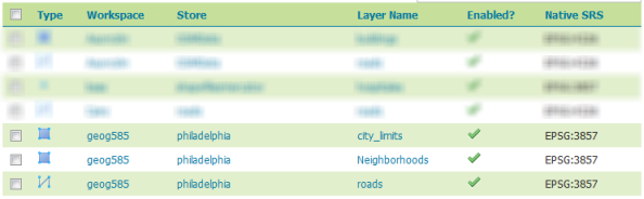 Figure 4.17 Layer list in GeoServer
 - Launch QGIS and add the Philadelphia/roads.shp and Philadelphia/city_limits.shp files as layers. Make sure you are adding the shapefiles, not the newly published WMS services.
Note: If the layers are vertically offset by 20 km, right-click each layer in the layer list and click Set Layer CRS. Then set the CRS to EPSG:3857. Even though you projected all these layers to EPSG:3857 using OGR, sometimes QGIS needs you to tell it to use its definition for EPSG:3857. - Style the city limits as a very light gray fill with no outline.
- Style the roads as a slightly darker gray, using a thin line (the default width is fine). You should have something like this:
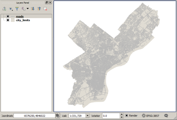 Figure 4.18 QGIS showing layers added
 - In the layer list, double-click the roads layer and choose the Symbology tab.
- At the bottom left, select Style > Save Style..., then select the "As SLD style file" option and save it anywhere as grayroads.sld.
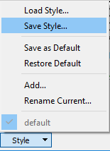 Figure 4.19 Save SLD dialog
 - Go back to the GeoServer Web Admin page and click Styles in the left-hand menu.
- Use the procedure from the previous walkthrough to create a new style called grayroads. As part of this process, upload the grayroads.sld file that you saved out of QGIS.
- Use the procedure from the previous walkthrough to apply your grayroads style as the default style for the Philadelphia roads layer that you have published in GeoServer. Preview your layer in OpenLayers to ensure the styling was applied as expected.
The above steps are significant because you were able to achieve the desired styling without editing any XML.
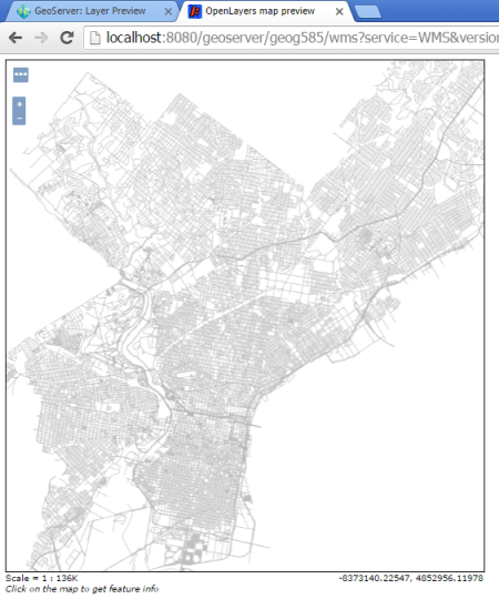 Figure 4.20 GeoServer preview of map layer
 - Repeat the above steps for the light gray city boundary style. Specifically, save the light gray polygon styling out as an SLD, create a style in GeoServer using this SLD, and then apply it as the default style for the city_limits layer. If you run into trouble, post a message on the course discussion forums.
Grouping multiple layers in a WMS using GeoServer
In some cases, you'll use WMS for your thematic layer and lay it in on top of a non-WMS basemap that uses tiles. This is what you did in the previous walkthrough. In some cases, when you have a very simple map, you may use a WMS for both the thematic layers and the base layers. Let's take a look at how GeoServer allows you to group multiple layers together in a single WMS. We'll use the neighborhoods layer, the city boundaries layer, and the roads layer that you have already published and styled in your geog585 workspace.
- Open the GeoServer Web Admin page and click Layer Groups in the left-hand menu.
- Click Add new layer group.
- Set up the first four properties as follows:
Name - NeighborhoodMap
Title - Philadelphia Neighborhood Map
Abstract - Map of Philadelphia neighborhoods using data derived from Zillow.com
Workspace - geog585 - Scroll down, and add your three layers using the Add Layer link. Use the arrows to put them in the order shown below. Notice that the top layer in the list is drawn first, the second layer in the list is drawn on top of that, etc., resulting in a layer list in reverse order from what you'd expect.
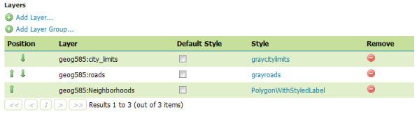 Figure 4.21 GeoServer Add Layer GUI
 - Scroll up a bit, and set the coordinate reference system to EPSG:3857. Then click Generate Bounds to calculate the bounding coordinates for the service.
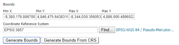 Figure 4.22 GeoServer Generate Bounds dialog
 - Go to the Tile Caching tab, and uncheck Create a cached layer for this layer group. Although GeoServer allows you to create a tile cache for this layer, we will focus on creating tiles in the next lesson using the superior drawing options of QGIS.
- Click Save. You should see your new group layer in the list. If you get a nullPointerException in GeoServer, proceed ahead with the next steps anyway, if you can. If they don't work, please check your previous steps and make sure everything was completed accurately, then post on the Technical Discussion Forum if you are still having issues.
- Use the Layer Preview link to preview your group layer in the OpenLayers viewer. You should see something like the styling below (note that I have zoomed in the preview from its initial extent).
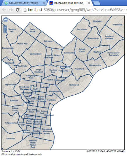 Figure 4.23 GeoServer preview of styled layer
 - Open a new map in QGIS, and connect to the group layer using the techniques from the previous walkthrough (click Connect again in the dialog box below to see an updated list of layers in your WMS). Remember to set the CRS to EPSG:3857.
The layer should appear in your QGIS layer list as a single entity:
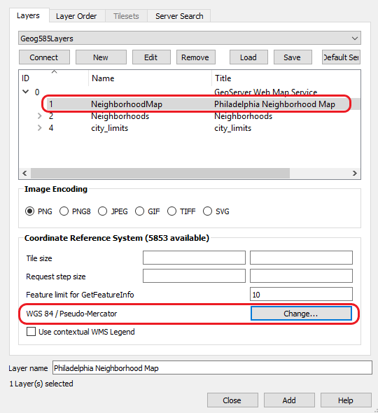 Figure 4.24 QGIS add WMS layer GUI
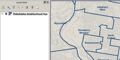 Figure 4.25 QGIS layer list sample
If you get an error when adding the layer, try cleaning out your QGIS WMS cache by clicking the Settings menu > Options, go to the Network tab of the options box, and then click the little red garbage can icon to clear the cache.
This exercise has shown how you can style any number of layers and group them together as a dynamically drawn WMS in GeoServer. If you have many layers to combine, it's faster and more scalable to use tiles, which you'll learn about in the next lesson. However, the techniques you've learned with WMS are sufficient to launch a quick and easy web map if you'll only have a few layers or a limited number of people using the map.
Lesson 4 assignment: Review a WMS and serve some of your term project data as a WMS
As you've completed the walkthroughs, you've hopefully begun to think about ways that you could serve your own term project data as a WMS. You are not required to use a WMS in your term project, but I would like you to get some more practice with it using your own data. If you like the result, you're welcome to use it in your term project submission.
The assignment this week has two parts:
- Write a short review of a public-facing WMS, namely the GEBCO WMS (General Bathymetic Chart of the Oceans; www.gebco.net [99]) with the URL https://www.gebco.net/data_and_products/gebco_web_services/web_map_service/mapserv? [100] . The accompanying web site for the WMS can be found here: https://www.gebco.net/data_and_products/gebco_web_services/web_map_service/ [101] . The review should include the following:
- the organization that published the WMS and the purpose of the WMS;
- the URL for a GetCapabilites request to that WMS;
- the technology (i.e., software) used to provide this WMS;
- a description of what layers are available in the WMS and in which formats (projections, image format, etc.);
- a screenshot of one of the layers opened in QGIS and some comments on the styling used for the layer.
- Using GeoServer and the techniques learned in this lesson, serve some of your term project data as a WMS, using a custom style you've made using the SLD Cookbook [90] or QGIS. This can be a single layer or a group layer, but it should use custom styling that goes beyond the GeoServer default style. To receive the final 1 point for this part of the assignment, it is expected that you manually edit the SLD code to realize one of the more advanced styling options not covered in the lesson that you can find in the cookbook (see rubric). Assemble a word processor document with a report containing the following:
- a description of the layer you served;
- a screenshot of the layer(s) in the GeoServer layer list;
- a description of how you made the style;
- a screenshot of the style page in GeoServer (including as much of the SLD code as possible);
- a screenshot of the WMS displayed in the OpenLayers preview;
Submit these deliverables to the Lesson 4 assignment drop box on Canvas, either as a single document or as two separate documents.
Lesson 5: Building tiled maps with FOSS
The links below provide an outline of the material for this lesson. Be sure to carefully read through the entire lesson before returning to Canvas to submit your assignments.
Note: You can print the entire lesson by clicking on the "Print" link above.
Overview
This week's lesson focuses on tiled web maps. Tiles are relatively small square-shaped "chunks" of data (either rasterized map images or raw vector coordinates) that have been pregenerated by the server and stored in a directory called a cache. When web users navigate the map, the server can just hand out the tiles rather than generating the map on the fly.
In this lesson, you'll learn the pros and cons of tiled maps, as well as strategies for building and maintaining a tile cache. You will learn about traditional rasterized tiled image formats, as well as a newer generation of tiles that store vector coordinates. Because rasterized image tiles have been around much longer and have mature support from tile generating engines, tile servers, and clients, most of the lesson content focuses on these types of tiles. The newer vector tile format is discussed near the end of the lesson content.
There are two walkthroughs associated with this lesson, both of which involve rasterized image tiles because these currently have the most mature tools for end-to-end FOSS workflows. The first walkthrough shows how to create a simple cache of your Philadelphia neighborhoods map using the GeoWebCache software that is integrated into GeoServer. In the second walkthrough, you'll use QGIS to create a Philadelphia basemap cache with some nicer cartography than you would get using GeoServer.
Objectives
- Describe the advantages of tiled web maps and identify when it is appropriate to use them.
- Recognize strategies and techniques for creating and updating large tiled web maps.
- Describe the differences between rasterized image tiles and vector tiles, and the reasons that each might be used
- Create tiles for a WMS using GeoWebCache.
- Use best practices in multiscale map design to create a tiled basemap using QGISl.
- Discuss hosting options for tiled maps. Unpack and upload your tiled map to your own webspace (on AWS).
Checklist
- Read the Lesson 5 materials on this page.
- Complete the two walkthroughs.
- Complete the Lesson 5 assignment.
Why tiled maps?
As mentioned in previous lessons, the earliest web maps were typically drawn on the fly by the server, no matter how many layers were available or requested. These are the types of maps you just created using GeoServer and WMS. As you may have noticed, the symbol sets and labeling choices for this type of map are relatively limited and complex to work with. In fact, for many years, web cartographers had to build a map with minimal layer set and simple symbols to avoid hampering performance. In many cases, a cartographer was not even involved; instead, the web map was made by a server administrator tweaking XML files that defined the layer order, symbol sizes, and so forth. This was the case with both open specification web services (like WMS) and proprietary web services (like Esri ArcIMS).
Part of this approach stemmed from early efforts to make web GIS applications look exactly like their desktop counterparts. Sometimes these are referred to as “Swiss Army Knife applications” because they try to do everything (you may know one!). People expected that in a web GIS they should be able to toggle layer visibility, reorder layers, change layer symbols on the fly, and do everything else that they were accustomed to doing on the desktop. Ironically, this mindset prevailed at a time when web technology was least suited to accommodate it.
In the mid-2000s, after Google Maps, Microsoft Virtual Earth (now Bing Maps), and other popular mapping applications hit the web, people started to realize that maybe they didn't need the ability to tinker with the properties of every single layer. These providers had started fusing their vector layers together in a single rasterized image that was divided into 256 x 256 pixel images, or tiles. These tiles were pregenerated and stored on disk for rapid distribution to clients. This was done out of necessity to support hundreds or thousands of simultaneous users, a burden too great for drawing the maps on the fly.
The figure below shows how a tiled map consists of a "pyramid" of images covering the extent of the map across various scales. Tiled maps typically come with a level, row, and column numbering scheme that can be shared across caches to make sure that tile boundaries match up if you are overlaying two tile sets.
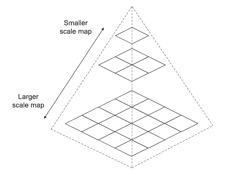
Cartographers loved the tiled maps because now they could invest all the tools of their trade into making an aesthetically pleasing web map without worrying about performance. Once you had created the tiles, you just had a set of images sitting on disk, and the server could retrieve a beautiful image just as fast as it could retrieve an ugly one. And because the tiled map images could be distributed so quickly by a web server, Google, and others were able to employ asynchronous JavaScript and XML (AJAX) programming techniques to retrieve the tiles with no page blink as people panned.
This was revolutionary. Which would you rather have: a slippy map with stunning cartography and no layer control, or a clunky and ugly map with the ability to reorder layers and adjust the color of a school? Some longtime GIS geeks had to stop to think about this, but for the common web user, the choice was a no-brainer.
Within a year or two of Google Maps' release, commercial GIS software began offering the ability to build map tiles. For many, ArcGIS Server was desirable because the map could be authored using the mature map authoring tools in ArcMap; however, cost was a concern for some. Arc2Earth was another commercial alternative. The free and open source Mapnik library could also build tiles, but it wasn't until recent years that projects like TileMill wrapped a user-friendly GUI around Mapnik. QGIS now also offers the option to create tiles, as you will see in the second walkthrough of this lesson.
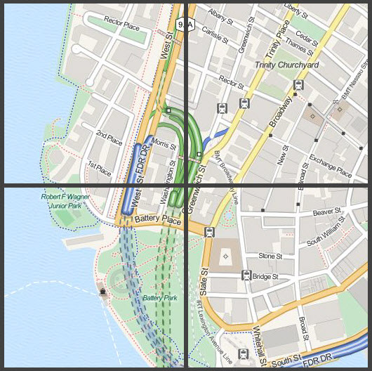
Tiled maps were the only model that could reasonably work for serving complex web maps to thousands of simultaneous users. However, they eliminated the ability for users to change layer order or symbols. People started working around this by serving out their general-purpose basemap layers as tiles and then overlaying a separate layer with thematic information. The general-purpose basemap tiles could be re-used in many applications. The thematic layers could also be tiled if the data didn't change too quickly or cover too broad an area at large scales. For example, you saw in Lesson 2 that the Microsoft Bing Maps traffic layer is served as PNG tiles.
Making the decision to build and maintain tiles
If you want faster navigation of your basemap, or you feel that more than a couple of users will be requesting maps simultaneously from your server, you should create a tile cache of your basemap. You may also choose to cache thematic layers if their features are not constantly changing attributes or position.
In both cases, be aware that the tile cache represents a snapshot of your data at the time the cache was created. To put it more bluntly, your tiles are “dumb images” that will not automatically update themselves when the back end data changes. You are responsible for periodically creating new tiles in order to update the map.
With large caches, sometimes server administrators target the cache updates at just the changed areas, rather than rebuilding tiles for the entire map. This requires keeping some kind of log about which places were edited, or comparing “before” and “after” versions of a dataset. Later in this course, you will see that OpenStreetMap.org works in this way. If you make an edit to OpenStreetMap, you'll see your changes appear within a few minutes (at least at the largest scales). This is not because the entire cache was rebuilt, but because an area of change was detected, thereby triggering a partial rebuild of the cache in just the modified area.
Is there an existing tile cache that meets your needs?
Building a tiled basemap requires lots of rich data, high-end map authoring software, cartographic skills, and potentially enormous amounts of time and disk space. You may still need to do it at one point or another, which is why you will get a taste of this experience in Geog 585. However, because of these challenges, general-purpose web mashups often use tiles made by somebody else. OpenStreetMap is an attractive option if you want free tiles with no restrictions. If you want to use Google's, Microsoft's, or Esri's tiles, you may be able to use them for free, or you may have to pay, depending on the nature of your map (commercial or not for profit) and how many people use your app. Other companies such as CloudMade and MapBox have marketed their own versions of tiles using OpenStreetMap data.
If you are going to build your own basemap, it's helpful to have an experienced cartographer on staff who is experienced with designing at multiple scales. The symbols, colors, and details must be adjusted appropriately at each of the scales where tiles are created. Tiled basemaps can quickly get complicated with layer and labeling scale suppression rules. Cartographers may also need to design one set of tiles to stand on its own and another set of tiles to overlay remotely sensed imagery, a task that requires very different colors and symbols.
Projection
If you are going to overlay your tiles with any of the tiles from OpenStreetMap, Google, Microsoft, or Esri (or even just attempt to look like them), you must warp your most precious GIS data into a modified spherical Mercator projection that was created solely for the convenience of fitting the world onto a set of square tiles. GIS purists balked at this idea and predicted it would fail to achieve mass uptake, but many people (at least at mid-latitudes) now hold their nose and move forward with it.
Be aware that Esri, Google, and other organizations have used other code numbers and variations of this projection in the past: things can get very confusing if you are using older software or APIs. In the past couple of years, people seem to have standardized on EPSG:3857 although even the subparameters of this projection can be interpreted in diverse ways that lead to offsets. As a side note, can you figure out the humorous reason that Google once used the code 900913 for this projection?
Even when you display your maps in EPSG:3857, you do not ever want to perform measurements in this projection. The results will be largely skewed even at mid-latitudes. It's best to make sure that geometries are projected into a more local coordinate system before performing any measurements. Most popular mapping tools such as Google Earth and the ArcGIS.com map viewer do this behind the scenes when you use their measuring tools, but it doesn't happen automatically if you're building your own solution.
Scales
Not only must you match the projection in order to overlay, you must also match the scales. These are not nice, well-rounded numbers; rather, they were derived mathematically from the starting point of putting the whole world on a 2x2 grid of tiles. For example, one of the scales is 1:36,111.98 and as you zoom in, the next one is 1:18,055.99. So much for your simple USGS 1:24000 series! Partly for this reason (and partly because many laypeople don't understand map scales), the common web map scaleset is often referred to with simple numbers such as “Level 14,” “Level 15,” etc., that increase as you zoom in. You just have to get a feel for which levels correspond to national scale, provincial scale, city scale, neighborhood scale, etc. The table in the Bing Maps Tile System [103] article is helpful for this.
Strategies for creating and serving map tiles
Map tiles often have a simple folder structure, which makes them easy to serve. However, they can become complex to manage due to their sheer size and number. There are several different ways people have devised to serve map tiles:
- Put them in a folder structure on your web server, and let people pull them directly. In this approach, you just organize the tiles as individual image files under a folder structure representing the scale level, row, and column. Many mapping APIs can use tiles when presented with a URL structure with variables representing the consistent position of the level, row, and column. For example, when using a tiled layer in the Leaflet API, you must provide a URL in the form http://{s}.somedomain.com/blabla/{z}/{x}/{y}.png, where z is the zoom level and x and y are the column and row.
- Make the tiles available through a web service. In this approach, the web service exposes parameters for you to request a tile based on a particular level, row, and column; however, the back-end infrastructure is a little more hidden. This approach has slightly more overhead (and therefore time lag) than exposing the tiles directly through a folder. A variation of the WMS specification called WMTS is designed for serving tiles and works in this manner. You can also see this pattern at work when you navigate around Google Maps using the network tool of your browser. The following tile URL for Google Maps reveals nothing about the back-end folder structure for the tiles, although you can see the level, row, and column variables at work if you look hard enough: https://mts0.google.com/vt/lyrs=m@241289412&hl=en&src=app&x=74&y=96&z=8&s=Galile [104]
Strategies for creating tiles
At large (zoomed in) scales, the number of tiles to cache can be overwhelming, especially if you are covering a broad area such as a state or country. The irony is that at such large scales, many tiles will convey very little information. Zooming in to a neighborhood block scale at 1:2250 may show plenty of interesting features, but pan out into the desert or ocean at the same scale, and the tile may be completely blank. Do you want to spend the hours creating these tiles and gigabytes of disk space to store them?
In these situations, you may want to find software that can create tiles on demand, meaning at the time they are first visited by a user. The first person to navigate to a region will need to wait for the server to create the tiles, but subsequent visitors will enjoy the full benefits of created tiles. The most popular areas will fill up with tiles, but you won't spend resources creating and storing tiles that are never visited. Obviously, this approach varies in effectiveness based on how fast the server can actually draw the tiles on demand.
An alternative is to use a “Data not available” tile to denote areas where tiles have not been created. Web map administrators are sometimes loathe to do this, but it is often a common enough practice that lay users blame themselves when they see the tile (“Oops, I zoomed in too far!”) rather than the administrator (“Why didn't they make the map available at this scale?”).
The best approach may be to strategically create a subset of the most interesting tiles and leave the less interesting tiles to be created on demand (or returned using a “Data not available” tile). As a geographer, it may hurt your soul to call any place “less interesting,” but the bitter truth is that not all tiles of the map experience an equal number of views. Fisher (2007) showed how early visitors to Microsoft Virtual Earth (now Bing Maps) stuck mostly to the big cities, coastlines, and transportation corridors. Quinn and Gahegan (2010) built models taking into account these patterns, showing how the majority of map requests could likely be satisfied by creating a fraction of the full number of tiles that it would ordinarily take to cover the full rectangular extent of the map. Their models were cobbled together using datasets like buffered roads, coastlines, and points of interests, but more recent feeds from social media such as geotagged tweets and Flickr photos may prove even more accurate in revealing the most interesting regions of the map for the majority of users. Note that some types of specialized maps (for mineral exploration, or wilderness conservation) may have very different usage patterns than general-use basemaps.
The ability to selectively cache a subset of tiles like this depends on the tile creation software's flexibility in allowing the administrator to designate custom regions for caching. Most software just allows the submission of a rectangular bounding box for tile creation; however, interesting areas of the map such as cities and coastlines are usually not shaped like rectangles. If you identify an irregularly-shaped region where you want to create tiles, you may have to abstract it into a series of rectangles and run multiple tile creation jobs, using each rectangle as an input. If you are luckier, your tile creation software will accept a spatial dataset (such as a shapefile) as a bounding region.
Creating tiles with FOSS
Creating tiled web maps is a common task that has been addressed by various FOSS packages. The most accessible one for you at this point is GeoWebCache because it's integrated directly into GeoServer. Others include TileCache and TileStache.
The Mapnik library is a FOSS tile creation library that binds to Python and other languages. It allows a lot of advanced drawing options not found in your typical WMS layer. Working with Mapnik typically required some Linux knowledge and some trial and error; however, the for-profit company Mapbox released an open source program called TileMill that can run on Mac and Windows and puts a nice GUI around Mapnik. We have been using TileMill in this class for a long time, but a couple of years ago, Mapbox stopped developing it. TileMill has been continued as a community-driven project on GitHub [105], but the development has slowed and problems have become more frequent recently. At the same time, tile creation support has been integrated into QGIS, so at some point, we made the decision to use QGIS for this part of the class as well. In the second walkthrough in this lesson, you'll use QGIS to create a basemap of Philadelphia using some of the layers you processed earlier.
References
- Fisher, D. (2007). Hotmap: Looking at geographic attention. Visualization and Computer Graphics, IEEE Transactions on, 13(6), 1184-1191.
- Quinn, S., & Gahegan, M. (2010). A predictive model for frequently viewed tiles in a web map. Transactions in GIS, 14(2), 193-216.
Vector tiles: the next generation of tiled maps
Although the rasterized tile sets we have discussed in this lesson are able to deliver nice-looking maps in a relatively rapid format, they can be cumbersome to keep updated, and they require enormous amounts of computing resources at large map scales. To work around these challenges, a data storage format called "vector tiles" has gained popularity in the past several years. Mapbox has led development efforts on vector tiles and has shared a vector tiles specification [106] under a Creative Commons license.
Vector tiles are exactly what you would guess: they store chunks of vector data instead of storing a map image. The idea behind vector tiles is that it is more efficient to keep data styling separate from the data coordinates and attributes. The client can use a predefined set of styling rules to draw tiles of raw vector coordinate and attribute data sent by the server. This allows the restyling of data on the fly, which is another serious limitation of rasterized tiles. Think about it: If you want to change the shade of green used to draw parks with your rasterized tiles, you must rebuild every tile containing a park. If you want to do the same thing with vector tiles, you just update your styling instructions in one place and the tiles themselves stay the same. Other display operations such as rotating the map also become easier to implement with vector tiles.
Vector tiles are designed to be small on disk, and employ a number of optimization approaches designed to reduce the amount of characters needed to store the geographic data and attributes, some of which are described in this video by Mapbox engineer Dane Springmeyer [107]. He also introduces a product called Mapbox Studio, [108] which works with vector tiles only and is being promoted by Mapbox as a replacement for Tile Mill. The .mbtiles file format, which originally stored rasterized tiles, now only stores vector tiles when exported from Mapbox Studio.
In reality, there continue to be use cases [109] for vector and rasterized tile formats, although it is likely that a number of organizations will see performance benefits from rebuilding some of their originally rasterized tile sets as vector tiles in the future. This is even more likely as popular commercial software packages such as ArcGIS introduce tools to work with the Mapbox vector tile specification, a strategic decision that Esri announced in a 2015 blog post [110]. On the open source side of things, GeoServer added support for vector tiles in version 2.14, as detailed in these instructions. [111]
Open source clients are also recognizing the staying power of vector tiles, exemplified by the VectorTile layer format [112] built into OpenLayers 3 and plugin support for Mapbox vector tiles in Leaflet [113]. At the time of this writing, QGIS does not natively support viewing vector tiles, although there is a relatively new plugin [114] for this purpose.
Walkthrough: Creating tiles with GeoServer using GeoWebCache
Suppose you're satisfied with the layers and symbols in your WMS, but you want it to draw faster and be available to many simultaneous users. In this situation, it might make sense to use GeoWebCache to create your tiles, because GeoWebCache is built directly into GeoServer. In this walkthrough, you'll use GeoWeb Cache to create a tile cache for the Philadelphia NeighborhoodMap group layer WMS that you published in the previous lesson.
- Start GeoServer and open the GeoServer Web Admin page.
- Use the Layer Preview link to preview your geog585:NeighborhoodMap group layer (the one with the green icon). Use the OpenLayers preview so that you can zoom and pan around. Take note of the performance and appearance of the map. You'll see the labels repositioned on each pan, a sure indication that tiles are not being used yet.
- In the GeoServer Web Admin page, click the Tile Layers link.
- Click the geog585:NeighborhoodMap link, and then select the Tile Caching tab. This is where you can set up parameters for caching of your layer. If you stopped here, your cache would be created on demand. In our case, we actually want to pregenerate tiles for most of the levels so that they won't need to be built on demand. GeoWebCache calls this "seeding" the cache.
- Click Tile Layers again and in the row for geog585:NeighborhoodMap, click Seed/Truncate.
 Figure 5.4 Tile Layers in GeoServer
 - Scroll down, and fill out the form to create a new task as shown in the image below. Notice that your tile creation task will create PNG images using the Google Maps tiling scheme (900913).
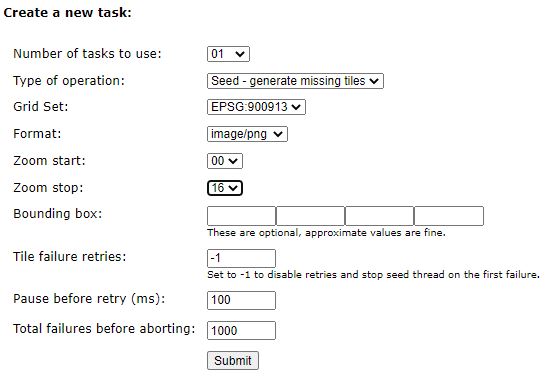 Figure 5.5 Tile Layers GUI in GeoServer
 - At the bottom of the form, click Submit. Although you can't see it, your computer is busy drawing your map over and over at different scales. This can tax the computer's memory and CPU resources, and you may see a performance impact on other applications while the caching is occurring. If you want to see your processor at work, open Windows Task Manager and look at the CPU and memory resources being used by java.exe.
- Every 30 seconds or so, click the Refresh List link to see the progress of your cache. When you click this link and the task status disappears, it means your cache is complete.
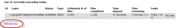 Figure 5.6 Tile Layers progress window in GeoServer
 - In the GeoServer Web Admin page, click Tile Layers and use the dropdown list to preview your cache in EPSG:900913 using the PNG format (see image below). This time when you pan around, you should see the map appearing instantly. You can verify that the tile cache is being used if the labels do not change position as you pan.
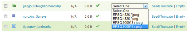 Figure 5.7 Tile Layers GUI for previewing the results in GeoServer
Caution: Make sure you are using the Tile Layers preview and not the Layer Preview preview. The Tile Layers preview uses a slightly different URL for the layer that indicates the tile cache should be used. Also, do not worry if the cache is reported on the Tile Layers page as N/A or 0.0 B in size. This seems to be normal, even though you have now built the cache.
Although performance is improved with the tile cache, you may notice some duplicate labels appearing. This is a difficult problem to avoid with map tiling, because each tile does not "know" about the labels on the adjacent tiles. To mitigate this problem, tile caching software typically draws an area much larger than a tile and then cuts it up into individual tiles. GeoWebCache calls this large area a "metatile" (Esri calls it a "supertile"). If you like, you can experiment with adjusting the metatile size; although duplicate labels can still appear at the metatile boundaries, the duplicates will be fewer and farther between. You may also find that the settings and options in the next walkthrough with QGIS make it easier to get the labeling you want.
Walkthrough: Creating tiles with QGIS
In this walkthrough, you will use QGIS to create a general-use basemap of Philadelphia. The idea is that you will be able to overlay thematic layers on top of this map in lessons to come. The data for this walkthrough is the base data for Philadelphia that you preprocessed in Lesson 3. If you followed all instructions, you should have this data in a folder called c:\data\Philadelphia or something similar. It should be using the mercator projection EPSG:3857.
Designing the map using QGIS
- Open QGIS, start a new project, and add the city limits shapefile. The projection of the project shown at the bottom right should automatically change to EPSG:3857.
- Open the Layer Styling panel, and change the symbol layer type from Simple Fill, to Outline: Simple Line.
- Change the Stroke width to 3 Points.
- Click on the current apllied color, and change the HTML notation (the hex code of a color) to #88789e.
- Hit Apply and close the Layer Styling Panel.
- Add the waterways shapefile to the project.
- Following the same process as above, change the color of the default SImple Line symbology to #89aceb.
- Change the width to 1 Point.
- Hit Apply and close the Layer Styling Panel.
- Add the natural features shapefile to the project and change the order of layers such that waterways is above natural features.
- Open the Layer Styling panel for natural features, and change the type from Single Symbol to Categorized.
- Use the drop down box below to assign the category value as type.
- Click the Classify button below to see all the available values of type.
- Change the colors for parks and forests to #ae8, and for reverbanks and water to #89aceb. After hitting apply, your map should look similar to this:
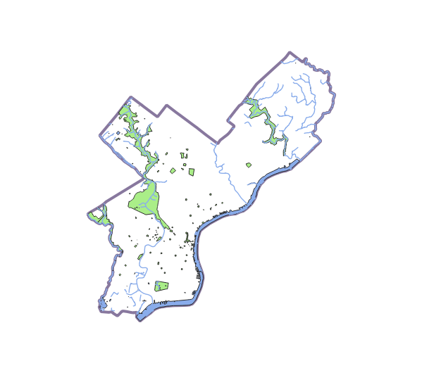 Figure 5.8 Progress so far.
 - Add the Neighborhoods shapefile to the project.
- Open the Layer Styling panel.
- Click on Simple Fill, and change both FIll color and Stroke color to tansparent. You can also turn the opacity all the way down to 0% to achieve the same result. This is because all we want from this layer are labels with the names of the neighborhoods.
- Hit Apply, and select the labels tab
 .
. - Change the No Labels option to Single Labels.
- Verify that the Value is set to NAME.
- On the first tab below called Text, change the font to Arial Black, size 12, color: #88789e.
- Select the furthest to the right tab called Rendering
 .
. - Enable the Scale Dependent Visibility, and set the minimum scale (the one with the minus on the magnifying glass) to 1:100,000.
- Hit Apply and close the Layer Styling panel. The result should look similar to the image below and the labels should disappear when you zoom out.
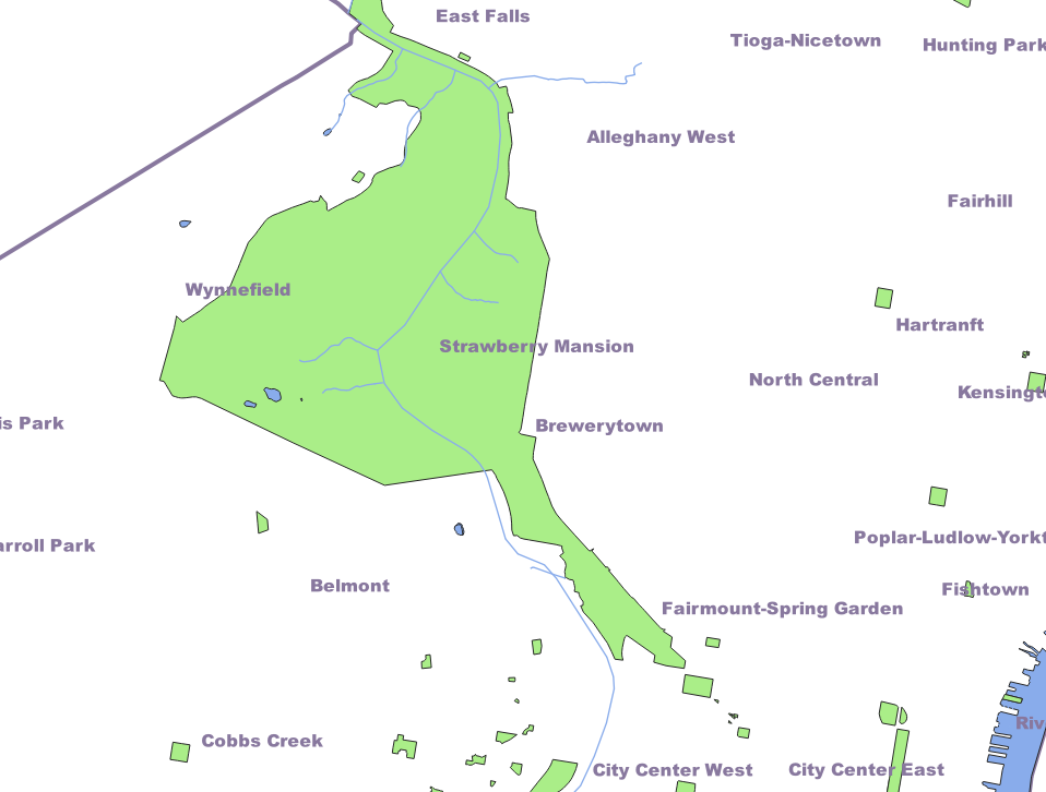 Figure 5.9. Neighborhood labels.
 - Add the roads shapefile to the project and rename it to Major Roads. The idea here is that we want minor roads to only show up at higher zoom levels. We will achieve this by setting up this new layer, to only show major roads and then later in step 30, add the roads layer to the project a second time to show all roads but with scale-specific rendering rules.
- Open the Layer Styling panel, and change the symbology to Categorized.
- Change the value to Type, and click Classify.
- Unselect all types but the following and set the color and width attributes as listed:
- motorway. Color: #606060, width: 3 Points.
- trunk. Color: #606060, width: 3 Points.
- primary. Color: #838383, width 2 Points.
- Click Apply and close the panel.
- Add the roads shapefile again and move it to a position directly below the Major roads layer in the Layers list so that major roads will be rendered on top.
- Open the Layer Styling panel.
- Set the color to #b6b6b6 and the width to 1 Point.
- Click on the labels tab, select Single Labels, and make sure that value is set to name.
- Change the font to Arial, size 11.
- Change the color to #b6b6b6.
- Go to the rendering tab, and enable the scale visibility.
- Set the minimum visibility to 1:25,000.
- Click apply and close the panel.
- The scale visibility in step 37 only applies to the labels, so we need to make the roads themselves only show up at a certain scale: Right click on the name of the layer, and select Set Layer Scale Visibility.
- Set the minimum visibility to 1:100,000. After clicking Ok, try out how the features and labels shown in the map change while you zoom in and out. Notice how minor roads only show up at higher zoom levels, and road labels are only starting to appear at even higher levels. The two images below give you an idea of how things should look like at low and high zoom levels.
One thing to note is that QGIS, in addition to applying the minimum scale condition for the labels, also by default applies a label layouting algorithm that will suppress labels of features that are very small at the current zoom level or would lead to overlap between labels. As a result, you will see even more road labels show up when you zoom in further. The technique of adding the same layer multiple times but with different settings is very helpful for implementing scale-specific rendering rules in the context of creating basemap tiles and in other application domains as well. We could have easily created a visual hierarchy with many more levels of features and labels showing up at different zoom levels but wanted to keep things relatively simple in this walkthrough. We also did not make much use of the more advanced approaches that QGIS provides for symbolizing vector layers, some of which you saw in the Lesson 1 walkthrough.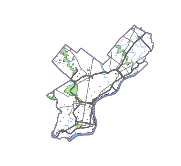 Figure 5.10 Map so far zoomed out.
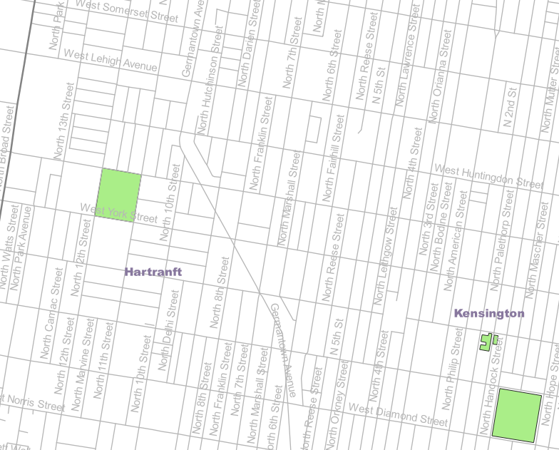 Figure 5.11 Map so far zoomed in.
 - Lastly, add the Railways shapefile to the project.
- Open the Layer Styling Panel.
- Change the color to #d2bcb0, and set the width to 1 Point.
- Before moving on, make sure the layers are arranged in the following order:
- Neighborhood
- City Limits
- Major Roads
- Roads
- Railways
- Waterways
- Natural
It would also be a good idea to save the project now!
Exporting the tiles
Once you've finished the map design phase and your map looks good at each scale, you can start thinking about generating the tiles. For large maps, plan for this to take some time, taking into account some of the factors discussed earlier in the lesson, such as the shape of the map and the scale levels you choose to generate.
This section of the walkthrough explains how to generate tiles of your Philadelphia basemap, and host them on the web. You will then test them out in a web page.
- Click the Toolbox icon on the top ribbon
 .
. - Search for xyz in the Processing Toolbox window that opens up.
- Select the tool named Generate XYZ tiles (Directory).
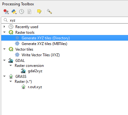 Figure 5.12 Generate tiles tool.
 - In the new window that opens, select the following options:
- Extent: click the button next to the box and select Calculate from Layer and select the City Limits layer (This determines the area for which tiles will be created. Some of the other options here can also be very useful, e.g., in cases where you don't have a suitable layer for deriving the extent from.)
- Minimum zoom: 0 (this is the lowest zoom level for which tiles will be created).
- Maximum zoom: 17 (highest zoom level for which tiles will be created).
- Tile format: PNG.
- Scroll down and select your desired Output directory by picking the Save to Directory... option and selecting a new folder that you created for storing the tiles called PhillyBasemap.
We are setting the minimum zoom level to zero here, so that tiles will be provided all the way up to the top of the pyramid in the tiles hierarchy. However, often when working with a relatively small project area like this (e.g., in your term projects), your plan is to limit how far out the user can zoom to avoid that the displayed area becomes tiny or (almost) invisible. In that case, it makes sense to set the minimum zoom option accordingly and use Javascript programming (see next few lessons) to restrict the possible zoom levels. That said, in terms of storage space, you won't save much by excluding the lower zoom levels because almost all storage will always be taken up by the highest levels.
- Press Run to create the tile images. Once this is done, check out the content of the output folder.
Hosting and testing the tiles
Setting up S3 storage and uploading tiles
If you navigate around your folder of tiles, you'll notice that the images are extracted into a highly organized structure of level\column\row. This structure is understood by various mapping programs and APIs, so all you have to do at this point is put your tiles onto a web-facing server. If you already have acces to some web space, you could simply upload the folder with the tiles to that web server. What we will instead do in this course is use Amazon's cloud services, namely the S3 service for scalable storage, as a convenient place to host the tiles on the web. We will place the tiles there and then test them in a web map. However, this will require you to set up an Amazon AWS account first, including registering a credit card. Uploading and accessing the tiles over the web will then cause some costs that your credit card will be billed for at the end of each month but these will be very small, < $10 most likely, if you just use the tiles for this class and follow the instructions below. The steps below will include descriptions of how to monitor the costs and how to set up a billing warning if the accumulated monthly costs go above a certain level. Please note that the workflow below is very specific to S3. If we would instead use a normal web server to host the tiles, we would most likely use FTP or SCP to upload the tiles to some folder in our personal web space on that server.
-
Go to: https://portal.aws.amazon.com/billing/signup [115]
-
Create a Root user account using your PSU email. (If you already have created an AWS account for your PSU email, e.g. for another class, you can instead log into that account and continue with Step 3.)
You can give your account any name you want. You will then have to verify your email address and define a Root user password. After that, you have to enter your contact information and confirm your identify by entering a verification code sent to you via SMS or an automatic call to the phone number you provide. Lastly, you have to select a support plan; please choose the free "Basic support plan". When done setting up your account, you can click the button that leads to the "AWS Management Console". -
Now, in the AWS Management Console, go to the search bar at the top of the screen and search for Billing . Click on the link (the name of the service at the top) to get to the "AWS Billing Dashboard".
 Figure 5.13 Amazon services search bar
 -
The Billing Dashboard will show you both a cost estimate for where you will end up at the end of the month and the current costs accumulated so far this month ("Current MTD balance"). Further down below, there is a link called "View your bill" which will lead you to a page where you can explore the costs accumulated so far by unfolding the items at the bottom under "Amazon Web Services EMEA SARL charge by service".
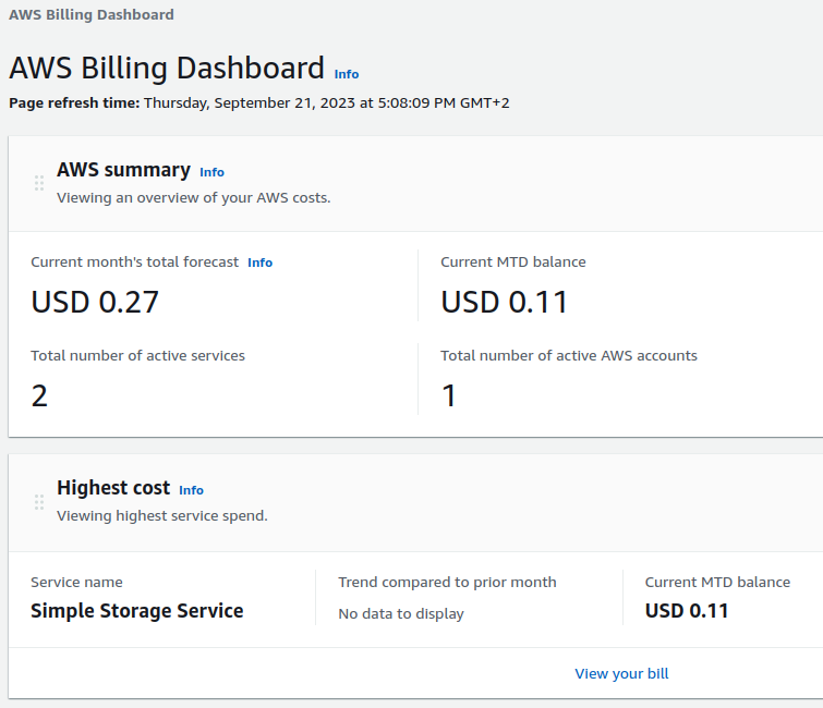 Figure 5.14 Amazon services billing information
 -
Now type in the term Budget in the search bar at the top and select the sevice called "AWS Budgets" by clicking the name. We now want to set up a budget so that you will get alerted by email if the estimated or accumulated costs for a month pass a certain threshold.
-
Click on the orange button "Create a budget" at the top. On the following page, select the options "Use a template (simplified)" and "Monthly cost budget", then fill out the details for the budget as shown in the image below but using your own email address to which the warning should be sent. The $5 is just a suggestion. Feel free to use a somewhat higher or lower number. You can also change the name of the budget but the default name is fine. Lastly, click the orange "Create budget" at the bottom.
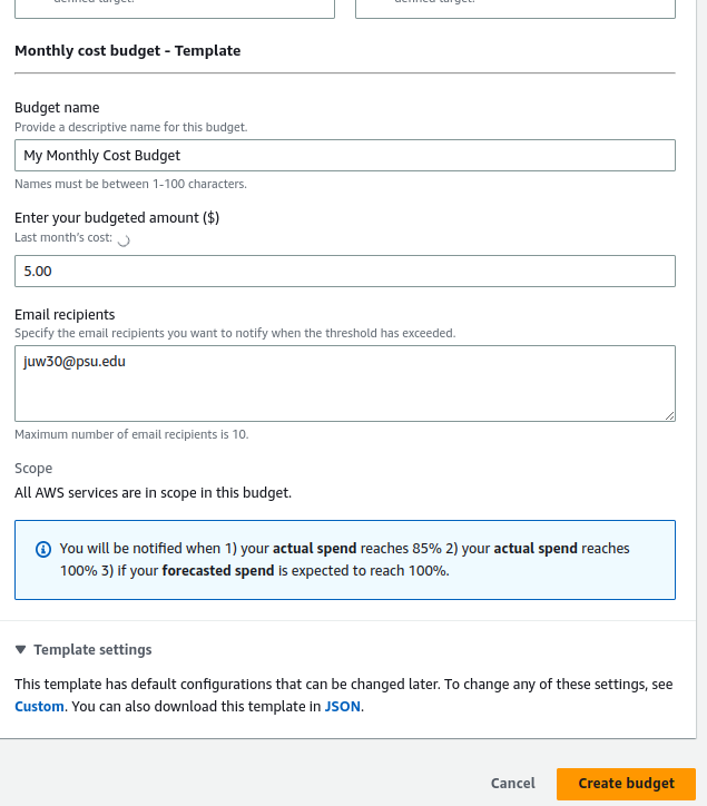 Figure 5.15 AWS creating the budget
As the information text said, you will now receive messages if any one of the following conditions is true: 1) your actual spend reaches 85% of the budget you defined, 2) your actual spend reached 100%, or 3) your forecasted spend is expected to reach 100% of the budget. You can alway go back to the AWS Budgets page to select and modify you budget there, including changing the threshold value. However, here is one important final note regarding the Billing and Budgets dashboards: For some reason, AWS does not update the accumulated costs in real-time. It can actually take multiple hours until the numbers get updated. Nevertheless, this should still help you keep track of how the costs are slowly increasing while you are using the data in your S3 bucket.
-
In the AWS Management Console, go to the search bar at the top of the screen again and now search for S3.
-
Click at the first result that is indeed the S3 service.
-
Once in the S3 service, click the orange button to create a bucket (basically a storage container inside your S3 cloud storage).
-
Under "General configuration", give your bucket a unique name, we recommend starting with "geog585-" followed by some random string of character and/or numbers that you pick yourself. We here will use the name geog585-a1rt15 .
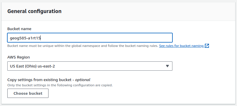 Figure 5.16 S3 bucket create
 -
If you want you can select the region that is closest to you, or in case of a real "global" project the region closest to your clients.
-
Scroll down to where it says Block Public Access settings for this bucket.
-
Usually we want to protect our data, but in this case, the map tiles have to be fully accessible by everyone, so uncheck the first tick to allow access.
-
Tick the box where you acknowledge that the bucket will become public.
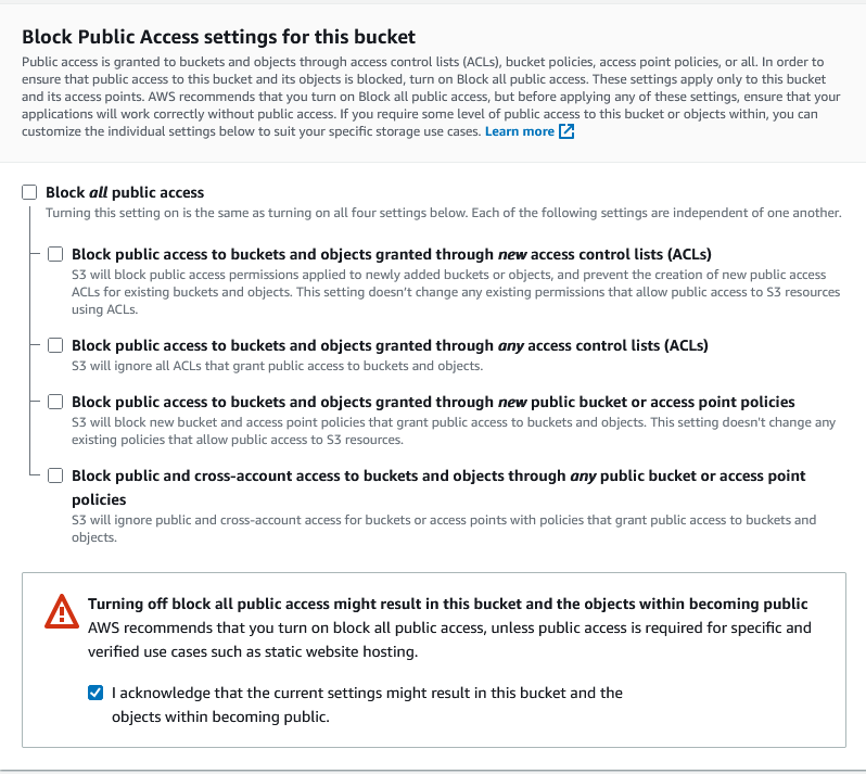 Figure 5.17 Bucket public access settings
-
-
Leave the rest as it is, and scroll down to click Create Bucket.
-
Once back to the main page, you should see your new bucket in the bucket list. Click on the name to open it up.
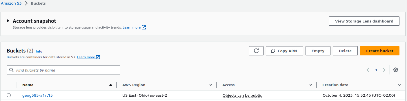 Figure 5.18 S3 Bucket List
 -
You should now see the page for your bucket, currently still not containing any objects. Click the tab called Permissions at the top.
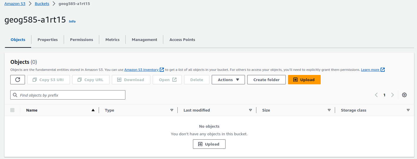 Figure 5.19 Bucket Page
 -
Scroll down to Bucket Policy and click Edit. Amazon really does not want us to create a public bucket unintentionally, so we need to do one more thing.
-
Copy and paste the following in the available space:
{
"Version": "2012-10-17",
"Statement": [
{
"Sid": "PublicReadGetObject",
"Effect": "Allow",
"Principal": "*",
"Action": "s3:GetObject",
"Resource": "arn:aws:s3:::geog585-a1rt15/*"
}
]
}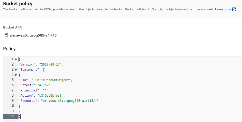 Figure 5.20 Bucket policy
 -
Above the text field and its title "Policy", you can find the ARN name of your bucket. Click the small icon left to it, to copy this name. Then go to the last line of the code you just pasted to change the name of the bucket there. Paste the ARN name you copied to replace the string arn:aws:s3:::geog585-a1rt15 there. Be careful to keep the initial double quote and the /*" after the bucket name.
-
Hit the orange button Save Changes.
-
Now we are almost read to upload our map tiles. If you only want to upload a couple of files (for instance, to upload and share the web map you will create in your Lesson 7 homework assignment), you can do so directly on the AWS page for your bucket by selecting the "Objects" tab at the top (you can think of "objects" as meaning "files" here) and then clicking the Upload button. This will show an area to which you can the drag and drop folder and files from the Windows File Explorer. The AWS will then scan the files and afterwards show you another Upload button that you can press to start the actual upload. However, this approach of using the web page won't work well for basemap tile sets that tend to consist of a huge amount of small files. The Philadelphia tile set, for instance, only is 200MB large in total but it consists of roughly 21,000 files. In our tests, uplading this amount of files via the web interface took around 6 hours.
Therefore, we are going to do the upload via another piece of software, the AWS Command Line Interface (CLI), which is much more efficient for small files and should be able to upload the Philadelphia tile set in just a few minutes. To set this up, we need to do two things: (1) Create a so-called Access Key that will allow us to access our S3 bucket via CLI and (2) install the CLI software itself. Let's start with creating a Root access key...
-
On the AWS page, click on your account name at the very top right of the page and then select "Security credentials". Scroll to the area called "Access keys". Then click the button called "Create access key".
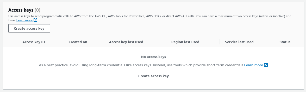 Figure 5.21 Creating access key
AWS will warn you that creating a Root access key is not the best practice. However, we want to keep things simple here, and you can always delete the access key immediately after you have successfully uploaded the files if you want. So please go ahead and enable the checkbox saying that you understand that this is not best practice, then click the orange button saying "Create access key".
-
AWS will now show you a window called "Retrieve access key" with your new access key in plain text and the corresponding secret key hidden by default. You can think of the access key as a login name and the secret key as the password. You will need both for using CLI, so please copy both of them. Important: This will be the only time you will be able to see/copy the secret key. If you loose it, you will have to go back and create a new access key. Once you have the keys stored somewhere else, click the "Done" button at the bottom. To delete or create further access keys, you can always go back to the Access Key area under Security Credentials as in Step 21.
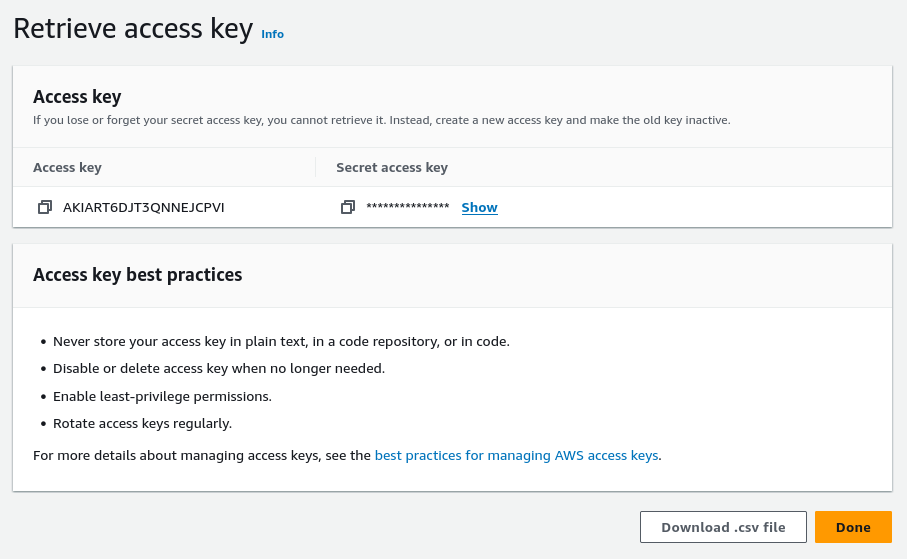 Figure 5.22 Access key and secret key
 -
Now, it is time to install the AWS CLI tools: Click on this link https://awscli.amazonaws.com/AWSCLIV2.msi [116] to download the software.
-
Double-click the downloaded file called AWSCLIV2.msi to start the installation. Then follow the instructions given by the installer.
-
Now open the Windows Command Shell cmd by going to the Windows start menu and typing cmd . This should open the black shell window (see next screenshot below in Step 27).
-
Let's first check if CLI has been installed correctly. Type in the following command and then press ENTER: aws --version
The output should look as shown in the next screenshot below starting with "aws-cli" followed by some version number. -
Next, we have to give CLI some information including the access key and secret key. Type in the following command and then press ENTER: aws configure
You will then be asked for access key, secret key, default region, and default format. For the access key and secret key, copy and paste the keys that you copied from the AWS page in Step 22. For the other two items, you can simply press ENTER without typing in antyhing.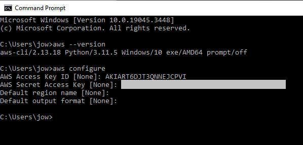 Figure 5.23 Configuring CLI
 -
Now we are ready to upload the files to our bucket. Use the cd command to move to the folder that contains the PhillyBasemap folder to which you exported the tiles in Steps 4+5 from the Section "Exporting the tiles" (see next screenshot from Step 29).
-
Now type in the following command but with the name in bold replaced by the bucket name you used and then press ENTER:
aws s3 cp PhillyBasemap s3://geog585-a1rt15/PhillyBasemap --recursive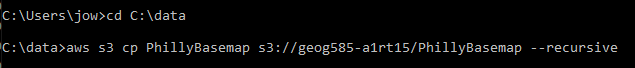 Figure 5.24 Starting the tile upload
 -
You should now see how the tiles are uploading. If instead you get some odd error messages. Try with running the command a second time; somehow this seems to happen sometimes on the first attempt.
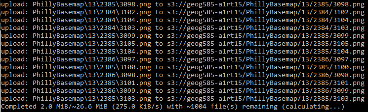 Figure 5.25 Tiles uploading
 -
Once everything is uploaded, you should see a prompt in the cmd shell window. Now switch back to the AWS web page and refresh the "Objects" tab on the page for your bucket. Navigate to the PhillyBasemp folder and then further into the subfolders to one random png tile.
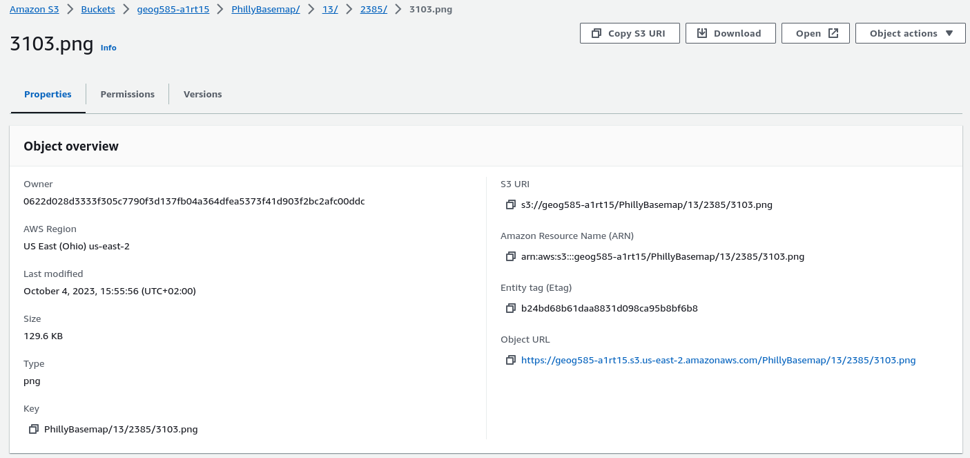 Figure 5.26 Object overview
 -
On the screen that opens, find the Object URL and copy it. The URL is made up of the base URL (https://geog585-a1rt15.s3.us-east-2.amazonaws.com/PhillyBasemap [117]) followed by the folders and file name corresponding to the zoom level and x, y indices of this particular tile image. If you want, you can open a new tab in your browser and copy the URL into the address bar to open this one tile. You should see the tile image but keep in mind that you have picked an empty tile so that you will just get an image that is fully white. To later use your basemap tiles in a web map you, you will have to take the base URL and then replace the concrete numbers at the end with a string of variabels to create a template string, for instance looking like this: https://geog585-a1rt15.s3.us-east-2.amazonaws.com/PhillyBasemap/ [118]{z}/{x}/{y}.png . We will make use of this option in the final part of this walkthrough in which we will test out our tiles in an ArcGIS Online map.
-
GOOD JOB! You are done!!
Testing the tile set in an ArcGIS Online map
- Open a browser to ArcGIS [119] and click the Map link at the top of the screen. You'll see an Esri-provided map, which we will switch out for our Philadelphia basemap. On the top right, select Open in Map Viewer Classic, so you can work and test your tiles without logging in.
- Click Add > Add Layer from Web. (If you don't see an Add button, first click the Modify Map link.)
- Choose to add data from A Tile Layer, and then populate the dialog box as shown below but using the base URL for the tiles in your own bucket from Step 32 in the previous section. Make sure to keep the /{level}/{col}/{row}.png part though. Note that ArcGIS Online uses different variable names (level, col, row) compared to the example given in Step 28 and what you will see in Leaflet in the next lesson. Also note that to set the extent, you must click Set Tile Coverage and draw a box around Philadelphia. You don't need to get the exact same coordinates shown below.
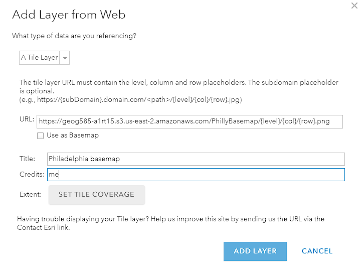 Figure 5.27 Add Layer from Web GUI in GeoServer
 - Click Add Layer. If nothing happens for a long time, repeat and make sure there is no error in the URL field. Navigate around your Philadelphia map to test it out. If you turn on the network utility of your browser's developer tools, you should be able to see the tiles being brought into the map.
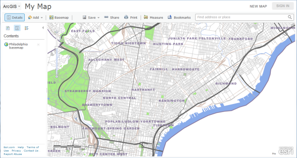 Figure 5.28 Sample map output
Optionally, you could add other web layers on top, but, for the sake of time, this will not be described here. In future lessons, you'll learn how to build this type of web map programmatically without using ArcGIS.com.
Lesson 5 assignment: Examine tiled maps, then build your own
Now that you've gone through a walkthrough and built your own tiled map, hopefully your appreciation has increased for the amount of cartographic design and effort required for producing a web basemap. In this week's assignment, you'll look at some existing tiled maps, then get some practice building your own.
Do the following:
- Find four online maps that use tiled maps in the background. These can be either rasterized image tiles or vector tiles. For each map, comment on where the tiles are coming from and how they were produced, if you can figure it out. It's okay if some of your tile providers are repeated (for example, two of the four might use Google Maps), but try to find at least one web map that uses a "homegrown" tiled basemap in the background. Simple local map viewers produced by city and county GIS websites are good places for this.
- Create a tiled map of rasterized images using some or all of your term project data. Depending on the nature of your data, this can be a basemap or a map with several thematic layers that is designed to overlay a basemap.
You should design this map using QGIS and upload it to your AWS S3 bucket, following the same procedures we used in the 2nd walkthrough. The map should be designed using sound cartographic principles, including aesthetically pleasing colors, an intuitive visual hierarchy, and a useful labeling scheme. Take advantage of scale-dependent rendering settings on your layers and the option of working with multiple copies of the same data set, so that the user is not overwhelmed with information at any particular scale. Zooming into the map should reveal progressively more information.
Important: Be careful with how many levels of tiles you build for this assignment, in particular if your project area is very large. Our recommendation is to keep the total size of the tile set that you are going to upload to S3 below 250MB, definitely below 500MB, and below 30,000 tiles in total (you can remove the subfolders for higher zoom levels after you produced the tiles to reduce the total size). As you saw in the walkthrough, if the project area is very small like a large city, a maximum zoom level of 17 should be ok. If your project area is an entire state in the U.S., try out what total sizes you get if you for maximum zoom levels between 12 and 14. If your project area is the entire U.S. (or a similar area), try out maximum zoom levels between 10 and 12. Also, if your tiled map consists of thematic layers, make sure the tile background is transparent, so that the tiles can be overlaid on top of other layers.
Please produce a report containing all the information requested in the first bullet above, as well as a URL to your tileset in your AWS S3 bucket so that I can test in a web map as shown in the walkthrough, together with a few words on how you designed your tiles so that I know what to look for. Then submit the report to the Lesson 5 drop box on Canvas.
Lesson 6: Putting layers together with a web mapping API
The links below provide an outline of the material for this lesson. Be sure to carefully read through the entire lesson before returning to Canvas to submit your assignments.
Note: You can print the entire lesson by clicking on the "Print" link above.
Overview
Note: Currently, this lesson teaches the Leaflet API. If you are looking for the earlier materials on OpenLayers, see the Lesson 6 archive page [120].
So far, you've been able to create several different types of layers, such as a dynamically-served web map service (WMS) and a static tiled web map. You've previewed these layers in various ways, but have probably come to the conclusion that they're not very useful or easy to share using these preview mechanisms. You will learn how to create more types of layers in future lessons, but, for now, we are going to pause for a week and learn how you can program a web application that combines your layers, creating an easily shareable "front end" for your web maps. You will learn what the Leaflet API is and how to use it for this purpose. It's impossible to learn Leaflet in a single week (or even in a single course), so, in this lesson, you'll just get a taste of the basics. Future lessons continue to use the Leaflet and expand on the knowledge you gain this week.
If you are new to web programming, it is recommended that you take some time to review the W3Schools HTML [121] and JavaScript [122] tutorials that you studied during orientation week. You don't need to know everything, but you do need to be familiar enough with the code and markup patterns that you can interpret most of what you are seeing when you view the examples later in the lesson. The prerequisite for this course is prior familiarity with at least one programming language, and it is expected in this lesson that you apply this familiarity to understanding the JavaScript syntax for loops, functions, decision structures, and so forth. Exerting a little extra time and effort, you should be able to see how JavaScript relates to the language(s) that you already know.
Objectives
- Identify commonly-used web mapping APIs (both proprietary and FOSS) and recognize programming patterns that are common to each.
- Choose developer examples that relate to your web mapping task and adjust the code to meet the needs of your own application.
- Use Leaflet to create a mashup from a tiled basemap and a WMS thematic layer.
- Create informational popups for your web map features using Leaflet.
Checklist
- Read the Lesson 6 materials on this page.
- Complete the walkthrough.
- Complete the Lesson 6 assignment (note that it has two distinct deliverables).
- Complete the "second quiz" on Canvas. This covers material from Lessons 4 - 6.
What is a web mapping API?
An API (application programming interface) is a framework that you can use to write a program. It provides a set of classes and functions that help you avoid writing all the low-level code to perform specific actions. For example, web mapping APIs typically include classes for maps and layers so that you don't have to write all the low-level code for displaying an interactive map image and drawing a new layer on it. Instead, you can just create a new map object, create a new layer object, and call some method such as layer.addTo(map). The API abstracts the complexity of the task and makes it easy for you to focus on the mapping aspects of your application, rather than spending time on the low-level logistics.
You've probably heard of general purpose APIs such as Java and the Microsoft .NET Framework that can be used to write all kinds of programs on desktop, web, and mobile platforms. There are also more specialized APIs built around certain products and functionalities. For example, you may have heard of Google App Engine, Amazon Web Services, and Microsoft Windows Azure that are designed for proprietary cloud computing environments.
APIs designed specifically for the purpose of making web maps include OpenLayers, Leaflet, the Google Maps API, and the ArcGIS API for JavaScript. The latter two are even more specific in that they are designed around particular proprietary platforms. This lesson introduces some of the different APIs and application development approaches, then gets into detail on how to use the Leaflet API.
Be aware that an API is not a programming language; rather, it is a set of building blocks that you invoke using a language. Some APIs are supported for use with multiple programming languages and other APIs are tied to one specific language. For example, there is both a language and an API named Java. The Java language is used to work with the Java API (and other APIs). In contrast, the .NET Framework is solely an API; there is no language called .NET. Applications using the .NET Framework are typically programmed using the C# or Visual Basic languages.
Choosing a web mapping API
When you set out to create a web map, one of the most important choices you will make is which API to use. If your application is large in scope with many clients, this one decision can affect your professional activities and trajectory for years. How can you select an API that will be the best fit for your requirements and skill set?
The selection of an API is often tightly coupled with the decision of a platform and programming language. These two factors affect the APIs available to you. For example, if you know that your application is required to run on Android tablets, you first need to decide whether you are going to build a full-fledged native app (in other words, one that is available in Google Play and has access to the device hardware such as the camera) or one that simply runs in a web browser on the Android tablet. Developing a native app most likely means that you'll be using Java, while developing a browser-based app allows more flexibility and can be done with JavaScript and HTML, perhaps employing an API that's designed to be mobile-friendly (in other words, it supports touch gestures, resizes to device width, and so forth).
From this example, you can probably also tell that it's important to consider which languages and platforms your developers are familiar with. If you have people on staff who know Java or Objective C, your options increase for developing native mobile apps. However, knowledge of HTML and JavaScript is usually sufficient to build browser-based apps. Most FOSS APIs for web mapping are geared toward an HTML and JavaScript approach, so this is what we'll focus on in Geog 585.
Examples of FOSS web mapping APIs
Below are some examples of FOSS web mapping APIs for building browser-based apps with HTML and JavaScript.
OpenLayers
OpenLayers [25] is a mature and richly featured JavaScript API for building web map applications. It has an extensive collection of documentation and samples, although some of the materials can be difficult for beginners to grasp. One of the nicest things about OpenLayers is the large developer community using the API. This community has created a mass of tips and examples on forums such as GIS Stack Exchange [123]. Although OpenLayers is not as approachable for beginners as some of the other APIs, its accumulation of online help resources, and its support for many layer types from both FOSS and commercial sources offer some advantage over other APIs. In 2014, OpenLayers 3 was released which was a major step because it was a complete rewrite of the library not compatible with the OpenLayers 2 branch anymore. In contrast, the current version OpenLayers 7 is still backwards compatible to previous versions of OpenLayers 3. If you feel comfortable with JavaScript and Leaflet after this lesson and decide you would like to use OpenLayers for your final project, you are welcome to go ahead, keeping in mind its strengths and weaknesses.
Leaflet
Leaflet [26] is a younger FOSS web mapping API that is designed to be lightweight, mobile-friendly, and easy to get started with. It has become extremely popular over the last years (one reason why we are now teaching it in this course), and quite a few companies, such as Mapbox, use it as a basis for their own APIs. Leaflet places heavy emphasis on the use of tiled maps and client-side vector graphics drawn from sources such as GeoJSON (you will learn more about the latter in the next lesson). For basic maps that use these layer types, Leaflet is an excellent choice that has already endeared itself to many GIS developers.
Leaflet contains a full API reference but only a handful of full working examples compared to OpenLayers. Going beyond the examples can be tricky for beginners; however, the simplicity of the API lends itself well to learning on the fly.
D3
D3 [28] is a FOSS data visualization library that is frequently used for charting, but also contains many map examples. It binds data elements to the page's document object model (DOM), allowing for interesting and flexible data animations and transitions. Although it has a steeper learning curve for newbies, D3 is a nice option for composing a web app with interactive maps and charts. It also offers examples for using non-Mercator projections [124].
Polymaps
Polymaps [29]is a simple FOSS mapping API primarily designed for mashing up map tiles with vector features drawn from GeoJSON and other sources. However, it seems like it is not under active development anymore, even though we have not seen an official announcement in this regard. Unfortunately, the developer examples on their web site also stopped working recently so that you can currently not see the map examples showing how Polymaps can transform and overlay a raster image [125] onto an existing tile set and demonstrating Polymap's unique ability to generalize a large set of points on the fly using k-means clustering [126].
ModestMaps
ModestMaps [27] is a lightweight FOSS API for displaying tiled maps. By design, it lacks a lot of the functionality of the other APIs mentioned above. Running JavaScript code requires transferring that code to the browser. Why load hundreds of functions if you know that you just want to display a map? Unfortunately, similarly to Polymaps, the web map examples on their pages don't seem to work anymore.
Examples of proprietary web mapping APIs
Several proprietary web mapping APIs created by commercial software companies have become very popular. In this context, "proprietary" means that the API's source code cannot be downloaded and/or is not permitted to be modified and/or cannot be deployed without paying a royalty.
I include this section on proprietary options because you will hear about them all the time, many are free to use (under various conditions), and some of them will work with the types of layers we're using in this course. Just be aware that proprietary APIs may be oriented toward the purchase of a particular product or service and may cost money if you deploy them for monetary benefit or if they incur enormous amounts of traffic. Always check the API's license agreement before you deploy any application on a server outside your own development machine.
Google Maps and Bing Maps APIs
The Google Maps API [127] part of the Google Maps Platform [128] gives developers the opportunity to overlay their own data on top of tiled map layers from Google Maps. The overlaid data is typically supplied through KML files, and is displayed as interactive vector graphics drawn on the client side. These graphics can be restyled by the developer to use custom marker symbols, and can be bound to popups or tables to show additional information on a mouse click.
Perhaps the biggest advantage of the Google Maps API is that it brings the look and feel of Google Maps to an application. Many Internet users have experience with Google Maps and may feel more comfortable when they see the Google Maps navigation control or map style, even when this is embedded in an unfamiliar third-party application. The Google Maps API is arguably no more robust or easier to use than some of the FOSS APIs described above; however, it is thoroughly documented and offers a large developer community.
In July 2018, Google Maps adopted a pay-as-you-go model wherein, all customers get $200/month of credit and must pay fees for service usage beyond this amount. Under their pricing plan at the time of this writing, that is enough to cover 100,000 static map views or 28,500 dynamic map views. See this page [129] for the most up-to-date information on Google's Pricing and Plans.
Microsoft's Bing Maps [130], another large commercial maps provider, offers APIs for web and mobile applications that are similar in scope to Google's. Bing Maps offers a free usage tier along with volume-based pricing for enterprises (see details here [131]). One difference from Google is that the Bing Maps API places less emphasis on KML usage, since Google popularized the KML format and is a primary platform used to create KML files.
The Google and Bing mapping APIs are a popular choices among developers of place-finder applications that display real estate listings [132], businesses [133], churches [134], etc. However, some sites are beginning to adopt FOSS alternatives. For example, Craigslist [135] has adopted a Leaflet + OpenStreetMap approach when showing the results of real estate searches.
ArcGIS APIs
Esri has created APIs for building both web apps and native mobile apps, some of which are relatively rich in function compared to the Google Maps API and many of the FOSS APIs. The ArcGIS API for JavaScript [136] is one of the most fully featured and actively developed of these APIs.
The ArcGIS APIs are primarily designed to work with web services that you have published using ArcGIS Online [137] and ArcGIS Enterprise [138] (comprised of ArcGIS Server [139] and Portal for ArcGIS [140]). However, some of the APIs can also display OGC services, KML, and generic tiled map services (such as the one we built with QGIS). One of the more distinguishing advantages of the APIs is their ability to tap into web services originating from ArcToolbox that perform geoprocessing on the server. This is an area where FOSS solutions lack an equivalent GUI experience (see the section on WPS services in Lesson 8).
The APIs are free to use for development or educational use, but require a fee if you are selling the application or embedding advertising within it. Published here are Esri's terms of use [141].
If you are interested in learning the Google Maps API and/or the ArcGIS API for JavaScript, the Penn State course materials for Geog 863 [2] provide an excellent place to get started.
Other web mapping APIs
A multitude of other free and proprietary APIs have appeared over the years for doing pretty much the same things as the ones listed above. Some of them, such as Mapbox-GL.js [142] (previously Mapbox.js [143]) and the CARTO Maps API [144], are associated with cloud-based mapping and location services. Please take a detour to read this GIS Stack Exchange post [145] describing available web mapping APIs. You will refer back to the post when you complete this week's assignment.
Programming patterns with web mapping APIs
If you distinguish yourself within your organization as a person who can develop web maps, it's likely you'll eventually be called upon to use more than just one of the APIs described in the previous section. As noted, project circumstances and requirements can force the selection of different APIs for differing endeavors. As a programmer, it's important to understand the general structures, patterns, and architectures behind the APIs and languages you use, so that you can learn new ones on the fly. Technology is always changing, and you will limit your utility if you tie yourself to a single development mode.
The following section describes some patterns and features that are held in common among many (but not all) of the web mapping APIs described earlier. I include this section before diving into Leaflet, so that you get an idea of what things are not unique to Leaflet when we begin looking at the code. However, I also include example snippets to show how the concept is implemented in Leaflet.
Nearly all pages that use web mapping APIs include the following:
References to JavaScript files and stylesheets
Before you can get off the ground, your HTML page needs to include a <script> tag pointing at the web mapping API's JavaScript files. Be aware that the more JavaScript you are referencing, the longer it will take to load your page. Some APIs are slimmer than others (hence a name like ModestMaps) but may offer fewer features. When adopting one of the larger APIs, like OpenLayers, some developers build and reference their own smaller version of the API that contains just the functions they want to offer.
There are a couple of ways to reference the API. One approach is to download and host the API on your own server, thus minimizing load times and allowing you to customize the API. The second approach is to reference the API on someone else's server. Sites called content delivery networks (CDNs) specialize in hosting commonly-referenced APIs. This is what a CDN URL looks like for Leaflet, referenced within a script tag within the page head:
<script src="https://cdnjs.cloudflare.com/ajax/libs/leaflet/1.2.0/leaflet.js"></script>
In this course, we'll reference Leaflet through the CloudFlare CDN in this manner, for simplicity. This requires you to maintain an Internet connection while you are testing your code. Be aware that if you were developing an internal application, needed full control over the APIs hardware, or needed to customize the API in any way, you would need to download and host the API yourself.
Many web mapping APIs offer some stylesheets that can get you started with making nice-looking applications. You can reference these stylesheets in the form of CSS files, either by hosting them on your own server or using a CDN. You can bring a Leaflet stylesheet into your page from the CloudFlare CDN within the head using syntax like this:
<link rel="stylesheet" href="https://cdnjs.cloudflare.com/ajax/libs/leaflet/1.2.0/leaflet.css" type="text/css" crossorigin="">
The map div and object
When you want to put a map in your page, you will typically carve out some space using an HTML <div> tag. You then create a map object using the API and relate it to your div.
For example, with Leaflet, you can create a map div like this in the body of your page.
<div id="mapid"></div>
Elsewhere in your page, in your JavaScript code, you can create a Leaftlet Map [146] object and relate it to the div. The L.map constructor takes the div name as an argument (L stands for the Leaflet library here).
var myMap;
myMap = new L.map('mapid');
The map contains methods for getting the current layer set, centering the map, zooming to given coordinates, and so forth. In many web mapping APIs, the map is one of the most powerful objects. Whenever you adopt a new mapping API, take a look at the reference documentation for the map object to understand what it can do and the syntax for invoking the most common methods.
Layer objects
Most web mapping APIs provide ways to define layer objects, which you add to the map object one by one to create your mashup. It is very important to note that a layer, in this sense, could represent a web service such as a WMS or tiled service that itself contains many underlying data layers. However, you would only need one layer object to bring this type of web service into your map. Other layer objects that reference single data files, such as KML or GeoJSON, are simpler to conceptualize.
In many web mapping APIs, the layer is an abstract (or "base") class offering a set of common properties, and is exposed to the developer only through more specific classes. Take a look at the methods and events offered in Leaftlet's Layer [147] base class. These include methods to add and remove the layer from the map and manage elements like popups and tooltips. Now look at the properties of some of the more specific derived classes such as TileLayer [148], WMS [149], and GeoJSON [150] to see some of the more specific methods associated with these layer types. You will typically be working with the API help documents at this lower level; however, it is important to remember that you still have all the properties and methods of the Layer class available to you whenever you use any of these specialized layer types.
When you create a new layer in Leaflet, you're generally expected to provide the URL or file path containing the source data for the layer. The layer will not show up on the map until you call its addTo(...) method. Adapted from the Leaflet documentation, here's one way you could create a layer referencing a WMS and add it onto your basemap:
var nexrad = L.tileLayer.wms("http://mesonet.agron.iastate.edu/cgi-bin/wms/nexrad/n0r.cgi", {
    layers: 'nexrad-n0r-900913',
    format: 'image/png',
    transparent: true,
    attribution: "Weather data © 2012 IEM Nexrad"
});

nexrad.addTo(myMap);
Don't worry if the meaning of all the parameters above is not immediately apparent. The important thing is to recognize that the layer required you to supply a URL before it could recognize the WMS. You were also able to toggle a transparency option and supply attribution text for the layer.
If you call the addTo(...) method on some other layer, it will be placed on top of the first layer.
Many types of tiled layers include the tile zoom level, row, and column number in each URL. When you create these layers in Leaflet, it would not make sense to supply a specific URL, since this would only point to one tile. Instead, you supply a general format using {x}, {y}, and {z} for the column, row, and zoom levels, respectively. This is sort of like what you did when you added your tiles to the ArcGIS Online map viewer in the previous lesson.
// create and add OpenStreetMap tile layer
var osm = L.tileLayer('http://{s}.tile.openstreetmap.org/{z}/{x}/{y}.png', {
maxZoom: 19,
attribution: '© <a href="http://www.openstreetmap.org/copyright">OpenStreetMap</a>'
});
osm.addTo(map);Layer styling mechanisms
Layers that come already drawn by the server, such as tiled maps and WMS images, already have styling applied, but for layers drawn by the browser such as GeoJSON or GeoRSS, you must define how the layer will be styled. Web mapping APIs typically offer a group of properties that you can set on a layer like this to define how the browser should draw it. These properties include things like fill width, fill color, outline width, outline color, and so forth. In Leaflet, it's common to define styles as functions that can then be referenced in the layer constructor, like so:
function parkStyle(feature) {
    return {
        fillColor: '#FF00FF',
        fillOpacity: 1,
        color: '#B04173',
    };
}

var gardenLayer = new L.GeoJSON.AJAX('gardens.geojson', {
    style: parkStyle
});

gardenLayer.addTo(map);
The style function returns a set of style properties (fillColor, fillOpacity, and color in this case) that will be applied when drawing the features from the layer. In this simple case, all features will look exactly the same. However, since the style function has the feature to be drawn as a parameter (function parameter feature), we can use properties of the feature to calculate its style property values. e.g., to have all features colored differently based on one of their attributes. You will learn how to do this later on in this course.
Many APIs allow you to use a custom image for a marker, rather than placing a simple dot. The Leaflet example below shows how you could add a GeoJSON layer of grocery stores to your map and style it with a shopping cart icon saved in an SVG (scalable vector graphics) file called grocery.svg. This could just as easily be a PNG file or other rasterized image type.
// create icons for supermarkets
var groceryIcon = L.icon({
    iconUrl: 'grocery.svg',
    iconSize: [20,20]
});

// create a vector layer of grocery stores from GeoJSON data
var groceryLayer = new L.GeoJSON.AJAX('supermarkets.geojson',{
    pointToLayer: function (feature, latlng) {
        return L.marker(latlng, {icon: groceryIcon});
    }
});

groceryLayer.addTo(map);
The result might look something like this when put on top of a basemap layer:
Don't worry if all the code above is not completely clear to you yet. Just make sure you can see where the style is being defined via a JavaScript object. In Lesson 7, you will get some more exposure to GeoJSON and styling browser-drawn graphics.
Events and interactive elements
Web mapping APIs offer interactive elements that help your map become more than just a static picture on an HTML page. The map and layer objects described above typically allow you to run code in response to certain user actions, such as clicking the mouse. The user action is called an event (or firing an event). The code you run in response is called the event handler, and it typically goes into its own function block of code. Sometimes the event can supply arguments to the handler function via an "event object" containing properties of the event, such as the screen coordinates of the mouse click that fired the event.
For example, you might instruct the map to "listen" for a mouse click event. You could then write a handler function that takes the screen coordinates of the event argument (in other words, the coordinates of the clicked pixel) and converts them to map coordinates, then writes the coordinates into a label in the HTML page so they can be seen by the user. An even greater measure of interactivity could be achieved by wiring up this handler function to a hover event, instead of a click. You would then get the effect of always seeing the coordinates of your mouse as you moved it around the screen.
Web map users often want to obtain more detailed information about specific features in the map. It is very common to handle a click event by showing a popup window with more information about the clicked feature; so common, in fact, that many web APIs have special classes and methods for popups that don't require you to write the typical amount of event listening logic. You will learn more about popups in Leaflet in future lessons in this course.
Sometimes popups are too limited in space or complexity for the content you want to show. Even if your mapping API allows you to cram large images or tabbed interfaces into a popup, it often makes more sense to show this type of content in an HTML div elsewhere on the page. Web mapping APIs allow you to perform queries on a clicked point and retrieve attribute information from the clicked features (often as part of a handler function like the ones mentioned above). You can then do anything you want with this handler function in order to display the information in HTML. You might even pass the information to a different specialized API that draws charts, queries Wikipedia, finds nearby homes for sale, and so forth.
Another common piece of desired interactivity is the ability to switch layers off and on. Remember that in this sense, a "layer" is an entire web service. It is obviously not possible to toggle the visibility of individual sublayers inside a tiled map because all the layers are "burned into" the tiled image. However, you could switch to a different tiled base map, or turn off a WMS or GeoJSON layer placed on top of it.
Leaflet offers a Layers Control [151] that acts like a table of contents for toggling visibility. You create your layers as usual, but instead of adding them to the map individually, you organize them in JavaScript objects for your base layers and overlays (thematic or business layers). Suppose you have two layer variables, grayscale and streets, representing tiled maps, and one layer variable cities representing a layer of city points. Again, from the Leaflet doc, here is how you can add the layer switching control with these defined as base layers and overlays:
var baseLayers = {
  "Grayscale": grayscale,
  "Streets": streets
};

var overlays = {
  "Cities": cities
};

L.control.layers(baseLayers, overlays).addTo(map);
Now that you are familiar with the different elements of a web mapping API and have seen how these are expressed in Leaflet, we'll move forward and take a look at some fully functioning examples.
Examining some Leaflet examples
Now that you have received an introduction to web mapping APIs and their basic elements, you need to start experimenting with one in order to make any more significant progress. The way you will learn Leaflet, and any other API, is by taking a look at its developer code samples, trying to run them, and experimenting with adjustments or tweaks to suit your fancy. Indeed, a strategy for building any web application is to find the combination of samples that best approximates what you want to do and then start experimenting with merging those samples, testing the functionality one piece at a time until you've met all your requirements.
In this spirit of exploration and experimentation, we are going to take some time to look through some of the Leaflet developer samples and other online supplementary materials such as developer forum posts. These are the kinds of resources that you'll be working with as you complete your final project and continue Leaflet development beyond this course. I want to make sure you can use and interpret them effectively.
In the next section of the lessons, you'll complete a walkthrough where you put your PhillyBasemap tiles that you made with QGIS into the map, and then place a WMS on top of them. The user should be able to click a feature in the WMS and see a popup with basic information about that feature. The completed walkthrough will look something like this:
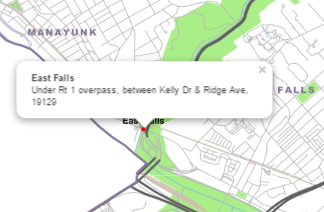
A good strategy when you approach a coding problem like this is to make a basic list of the things you'll need to figure out how to do. Then you can hunt for examples that show how to accomplish those tasks. In the above scenario, I can think of four key things you need to know how to do in order to get this to work.
- Add a tiled basemap to the map
- Add a WMS layer on top of the basemap
- Query a WMS layer on a mouse click
- Display the result in a popup
Now take a look through some of the following Leaflet examples and developer forum posts that could help you achieve this goal. Don't worry about writing the code yet; that will be covered in the walkthrough. For now, just get familiar with the code structure and patterns. Then the material will be somewhat familiar when it's time to complete the walkthrough.
Add a tiled basemap to the map
This is such a common task that you could go to the Leaflet Quick Start Guide [152] example. Indeed, this shows how to add a tiled basemap from Mapbox, using the L.tileLayer class:
L.tileLayer('https://api.tiles.mapbox.com/v4/{id}/{z}/{x}/{y}.png?access_token={accessToken}', ...)This is even more complex than you need, though, because the sample requires you to have a Mapbox access token and project ID. If you're just adding tiles hosted from your own server, you could adapt the simple code snippet from the L.tileLayer [153] API reference:
L.tileLayer('http://{s}.somedomain.com/{foo}/{z}/{x}/{y}.png', {foo: 'bar'});In this situation, foo just represents additional options you can apply to the tile layer. The important part is that you pass in a URL to your tiles with {x}, {y}, and {z} representing the column, row, and zoom level, respectively.
If you Google OpenStreetMap in Leaflet example, you'll find helpful sample code on the Getting Started with Leaflet [154] page that adds OpenStreetMap as a tiled basemap.
// set up the map
map = new L.Map('map');

// create the tile layer with correct attribution
var osmUrl='http://{s}.tile.openstreetmap.org/{z}/{x}/{y}.png';
var osmAttrib='Map data © <a href="http://openstreetmap.org">OpenStreetMap</a> contributors';
var osm = new L.TileLayer(osmUrl, {minZoom: 8, maxZoom: 12, attribution: osmAttrib});

// start the map in South-East England
map.setView(new L.LatLng(51.3, 0.7),9);
map.addLayer(osm);
Add a WMS layer on top of the basemap
The Leaflet examples contain a page about working with WMS in Leaflet. From the Leaflet WMS and TMS tutorial [155]:
var wmsLayer = L.tileLayer.wms('https://demo.boundlessgeo.com/geoserver/ows?', { layers: 'nasa:bluemarble' }).addTo(map);The above example shows how the L.tileLayer.wms [149] class can be used together with a URL and a list of layer names to add a WMS to the Leaflet map.
Query a WMS layer on a mouse click
This one is a little harder. A WMS query is based on a GetFeatureInfo request, and Leaflet doesn't provide any kind of method for doing that. In contrast, Leaflet is more focused on working with vector data drawn by the browser from sources like GeoJSON. Its support for WMS layers is limited to display only.
So how do you query a WMS using Leaflet? It's time to head over to Google and try WMS GetFeatureInfo Leaflet. A couple of resources in the results are useful. First, a GitHub page by Ryan Clark [156] shares some JavaScript functions he wrote for doing the GetFeatureInfo request directly through the web via jQuery and AJAX. I'll describe this more thoroughly in the walkthrough, but basically, he constructs a JavaScript string variable of the URL he needs in order to do the request, then he sends the request to the web using a method from the jQuery open source JavaScript helper library. Paul Crickard III wrote a simplified implementation [157] of Clark's technique on his blog that forms the basis for the code in the walkthrough.
Both examples listen for a mouse click event on the map to trigger the query, although this is coded in slightly different ways. Crickard's pattern is sufficient for our purposes, with onMapClick being a function that runs after the map detects a click event:
map.addEventListener('click', onMapClick);
function onMapClick(e){
  . . .
}
Please take a few minutes to review both these resources and do your best to see what's going on. You likely won't understand all the code, but pay attention to the general patterns of setting up a URL, making a request, and working with the result.
Display the result in a popup
Both Clark's and Crickard's GetFeatureInfo examples above display elements of the query response inside a popup. Both use the L.Popup [158] class for this, but Crickard's example is a bit easier to follow for beginners. He does:
popup = new L.Popup({maxWidth: 400});
Then later he sets an anchor point for the popup and the content that should appear inside.
popup.setLatLng(e.latlng);
popup.setContent("<iframe src='"+URL+"' width='300' height='100' frameborder='0'></iframe>");
map.openPopup(popup);
Notice that HTML can be used for the content. You can parse the WMS GetFeatureInfo response and pull out the elements you need and format them into an HTML string to act as the content.
Finding and adapting examples to fit your goal
It's natural to ask, "How do you expect me to write a bunch of code like this from scratch when I'm just barely getting familiar with JavaScript?!" The answer is that you don't have to write code like this from scratch. You only need to know enough to interpret and adapt a working example. Using the documentation and examining the code line by line, you should be able to get at least a basic idea of what is happening. If there's a parameter you don't understand, you can zero in on it. But don't worry about grasping everything.
Experienced developers sometimes say that the way to learn an API is to "play with it." This can drive beginners insane. Play with what? How do I even know what to do? In this lesson, you have hopefully learned to pick out simple code examples that are most relevant to what you want to do, then examine them line by line and see if you can tell what each line of the code is doing. Then make minor adjustments to the code to fit it to your own data and scenario. (This is the "playing with it" part.) Let's go to the walkthrough to see how the above examples could be adapted to some of your own web map services.
Walkthrough: Overlaying a WMS on a tiled map with Leaflet
The goal of this walkthrough is to get some practice overlaying different kinds of web services in Leaflet. You will first publish a WMS showing farmers' markets in Philadelphia. You will then use Leaflet to place this layer on top of the Philadelphia basemap tiles you made with QGIS in the previous lesson. You'll also add code, so that a user of your application can click any farmers market and see some more information in a popup.
Setting up the farmers' markets WMS
The first step is setting up a (passably) good-looking WMS showing farmers' markets in Philadelphia. In this application, the farmers' markets WMS will play the role of the business layer.
Setting up this WMS will be a nice review of some of the skills you learned in Lesson 4. In places where step-by-step instructions are lacking, you should be able to go back to the Lesson 4 walkthrough to remember the procedures.
- Download this shapefile of Philadelphia farmers' markets [159]. This was obtained from the City of Philadelphia via the PASDA [66] library. It's probably easiest if you extract it into your C:\data\Philadelphia folder.
- Open the GeoServer web admin page, and publish the farmers market shapefile as a layer in GeoServer using coordinate system EPSG:3857. Put it into your geog585 workspace. It should look like the following when you preview the layer.
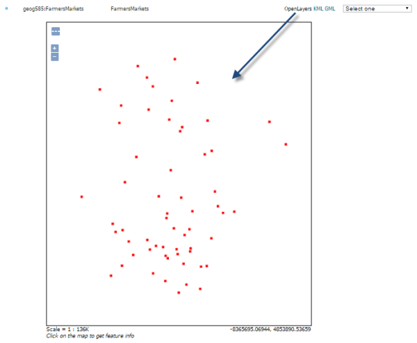 Figure 6.5
 - Using the SLD Cookbook example for Point With Styled Label [160], create an SLD named point_pointwithstyledlabel. If you don't remember how to do this, see the Lesson 4 walkthrough. You did exactly the same thing in that lesson using a polygon example.
Remember that the SLD is case-sensitive when reading the field that contains the label name. In this FarmersMarkets shapefile, the field you want to use for the label text is called NAME, in all caps, therefore, you will have to change the SLD code so that NAME is in all caps:<Label> <ogc:PropertyName>NAME</ogc:PropertyName> </Label> - Apply the point_pointwithstyledlabel SLD to your farmers market WMS so that it is the only available SLD, or at least the default. Again, see the Lesson 4 walkthrough if you're having trouble remembering how to do this.
When you have successfully applied the SLD, the WMS should look like the following when you preview the layer in GeoServer:You've now successfully prepared the WMS that you will overlay on your tiled map later in this walkthrough.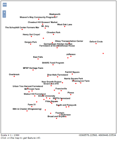 Figure 6.6
Preparing the web development environment
Now you'll make a few preparations for writing a simple Leaflet application. We’re going to host this app on the mini web server called Jetty that is installed with GeoServer. Just remember that in "the real world" you would probably get your IT staff to install an enterprise grade web server, such as Apache where you could run both GeoServer and your HTML pages. If you don't have an IT staff, you may even be lucky enough to do this yourself someday! :-)
- Stop GeoServer. (run the shutdown.bat file in the bin folder or press CTRL+C in the command shell window in which GeoServer is running than confirm with Y)
- Create a folder C:\Users\{username}\GeoServer 2.x.x\webapps\geog585 (insert your user name or adapt accordingly if you have installed GeoServer somewhere else)
- As you develop web pages, you will put all your HTML pages and stylesheets in this folder.
- Start GeoServer (run the startup.bat file in the bin folder)
As long as GeoServer is started, you should now be able to access your HTML pages through a URL such as http://localhost:8080/geog585/mypage.html [161] (where mypage.html needs to be replaced by the name of the actual html file).
Your HTML pages will often use stylesheets to define how the page should be drawn.
- Create a new text file and paste in the following code:
#mapid {
    width: 512px;
    height: 512px;
    border: 1px solid #ccc;
}

.leaflet-container {
    background: #fff;
}
The above CSS sets the size of the map container, the size and color of the map border, and the color of the background.
- Save the file in your new Jetty folder as ...\GeoServer 2.x.x\webapps\geog585\style.css. If you get an access denied error, you will have to modify the access rights of the geog585 folder so that your user has read and write access rights to the folder. Alternatively, you can try to run your text editor in Administrator mode.
- Test that your CSS is accessible by opening a browser to http://localhost:8080/geog585/style.css [162]. You should see the same CSS file.
If you get an HTTP 404 “Page not found” error and you are certain your URL is correct (or try it without the .css extension - http://localhost:8080/geog585/style [163]), then something might have gone wrong with Jetty recognizing your new geog585 folder. I have been able to work around this situation by doing a full restart of the machine and starting GeoServer again. After that, the folder was recognized.
Note that when you also put your HTML pages in this folder, you can refer to this file in your HTML code simply as style.css instead of supplying the entire URL.
- Save and close style.css.
Creating the HTML page and writing the code
Now you'll create an HTML page and insert the JavaScript code that configures the map and popups. The steps below do not provide the code linearly; you are expected to insert the code in the correct places as given in the instructions. Code is hierarchical, in the sense that some blocks run within others. It's more intuitive to describe the blocks of code rather than to give the code in its exact sequence. If you get confused about where the code is supposed to go, refer to the full example code at the end of this walkthrough page.
- Create an empty text file and save it as markets.html in your Jetty web folder (in other words, ...\GeoServer 2.x.x\webapps\geog585\).
Tip: If you are trying to edit this file later in the lesson and your text editor won't let you save it, stop GeoServer. You can start GeoServer after you have saved your edits and are ready to preview.
- Place the following code in your text file (unlike Python, indentation doesn't matter in HTML, so don't worry if the indentation doesn't come through exactly):
<!DOCTYPE html>
    <html>
      <head>
        <meta http-equiv="Content-Type" content="text/html; charset=utf-8">
        <title>Farmers markets in Philadelphia</title>
          <link rel="stylesheet" href="https://cdnjs.cloudflare.com/ajax/libs/leaflet/1.2.0/leaflet.css" type="text/css" crossorigin="">
        <script src="https://cdnjs.cloudflare.com/ajax/libs/leaflet/1.2.0/leaflet.js" crossorigin=""></script>
        <script src="http://ajax.googleapis.com/ajax/libs/jquery/1.9.1/jquery.min.js"></script>
        <link rel="stylesheet" href="style.css" type="text/css">

        <script type="text/javascript">


        </script>
      </head>
      <body onload="init()">
        <h1 id="title">Farmers markets in Philadelphia</h1>

        <div id="mapid">
        </div>

        <div id="docs">
            <p>This page shows farmers markets in Philadelphia, Pennsylvania. Click a market to get more information.</p>
        </div>

      </body>
    </html>
The above code contains the HTML head and body. This should give you a shell of a page, although you won't see the map show up yet.
In the head, notice the references to the Leaflet JavaScript and CSS files, both running on the CloudFlare CDN. There's also a reference to the style.css that you placed in your web folder earlier, which in some cases overrides the Leaflet stylesheet. Finally, there is a reference to the jQuery JavaScript library, which is running on Google’s CDN. jQuery is a helper library that greatly simplifies some JavaScript tasks. We’re going to use it here to make a web request to query the WMS, since there’s no easy way to do a WMS GetFeatureInfo request in Leaflet.
In the body, notice there is a div element with id "mapid" that is intended to hold our Leaflet web map. The CSS style for this element is defined in style.css and it sets the width and the height of the map in pixels. If you wanted to change the map width and height, you would modify the CSS.
When the body of the page has loaded, it runs the init() function from the JavaScript code we’ll add later. That’s why you see <body onload="init()">.
From this point on, we will not make any changes to the head or body. We will be inserting JavaScript logic in the <script> tag.
- Within the <script type="text/javascript"></script> tag, insert the following code:
var map;
function init() {
   // create map and set center and zoom level
   map = new L.map('mapid');
   map.setView([39.9526,-75.1652],13);
   . . .
}
This sets up a global variable named map that can be used throughout your JavaScript code. Then an initialization function called init() is defined, which you’ll recall is the function you set to run when the page body loads. The first thing the function does is instantiate a Leaflet map object within your mapid div. It then centers the map at 39.9526 N 75.1652 W at zoom level 13.
In this walkthrough, you will insert the remaining JavaScript inside of the init() function where you see the . . . above.
- Now you’ll add some code to bring in your Philly basemap tiles. Insert the following in the init() function of your code, directly after the line where you called map.setView().
// create tile layer and add it to map
var tiles = L.tileLayer('https://<URL of your S3 bucket>/PhillyBasemap/{z}/{x}/{y}.png');
tiles.addTo(map);
The above code creates a Leaflet tile layer that references your PhillyBasemap that you made with QGIS in Lesson 5. In the code above, you must modify the URL to use your S3 bucket name as created in the L5 walkthrough. The final URL should look something to this:
https://geog585-somestring.s3.someregion.amazonaws.com/PhillyBasemap/{z}/{x}/{y}.png
The URL to the tiles is provided in a generic format where z means zoom level number, x means column number, and y means row number. As long as you give Leaflet this tile URL structure, it will be smart enough to request the correct tiles as you pan and zoom around the map.
Notice how the tileLayer.addTo() method is used to add the layer to the map. The map object is passed in as a parameter. In some other mapping APIs like OpenLayers you call an add method on the map itself and provide the layer as a parameter.
- Add the following code immediately after the code you entered in the previous step:
// create wms layer
 var farmerMarkets = L.tileLayer.wms('http://localhost:8080/geoserver/geog585/wms', {
  layers: 'geog585:FarmersMarkets',
  format: 'image/png',
  transparent: true
});

farmerMarkets.addTo(map);

. . .
This adds the WMS layer of the farmers markets to the map. Notice how Leaflet’s wms class is used for this. You give it some properties such as the URL, layers, and image format you want (all using WMS-friendly syntax), and Leaflet takes care of formatting and sending the GetMap requests and displaying the responses as the user zooms and pans around the map.
So far, creating the map and adding the layers were pretty simple. It’s clicking the WMS and seeing a popup that turns out to be more complex. In order to do this, you have to send a WMS GetFeatureInfo request to the server. Leaflet offers no options for this, so you have to do it yourself by constructing a URL, sending it to the server, and reading the response. So how do you make a web request like this using JavaScript?
One way is by using jQuery, an open source API designed for simplifying things that JavaScript programmers have to do day in and day out. One of these tasks is sending web requests to a server while the end user is interacting with a web page (ie, clicking your map). The request is sent using a technique called AJAX (Asynchronous JavaScript and XML) which avoids a total page refresh.
With this in mind, let’s write an Identify function that we can fire off whenever someone clicks the map. This function will construct a WMS GetFeatureInfo request, send the request to the server using AJAX, and put the response into a popup.
- Add the following to your code directly after the lines you added above in the place of the . . .:
// define event handler function for click events and register it
function Identify(e)
{
  . . .
}
map.addEventListener('click', Identify);
Above is the Identify function that runs whenever you fire off a mouse event. I haven’t provided this entire function yet because it is long; however, I have inserted a … so you can see that together with the definition of this function, an “event listener” is added to the map to keep on the alert for any mouse clicks that occur. If someone clicks the map, the Identify function will be fired and a Leaflet event object [164] called ‘e’ containing some properties of the clicked point will be brought into the function.
- Replace the code in the … above with the following:
// set parameters needed for GetFeatureInfo WMS request
var sw = map.options.crs.project(map.getBounds().getSouthWest());
var ne = map.options.crs.project(map.getBounds().getNorthEast());
var BBOX = sw.x + "," + sw.y + "," + ne.x + "," + ne.y;
var WIDTH = map.getSize().x;
var HEIGHT = map.getSize().y;
. . .
Some key things we need in order to construct a GetFeatureInfo request are the bounding coordinates of the map, the width of the map in pixels, and the height of the map in pixels. The Leaflet map object provides ways of getting those properties. That’s what’s happening in the code above. The southwest and northeast corner coordinates of the map are retrieved, and these are formatted into a comma-delimited string in the syntax required by the BBOX parameter. Then the width and height are also retrieved from the Leaflet map.
- Continue filling in the Identify function by replacing the … in the code above with the following:
var X = Math.trunc(map.layerPointToContainerPoint(e.layerPoint).x);
var Y = Math.trunc(map.layerPointToContainerPoint(e.layerPoint).y);
// compose the URL for the request
var URL = 'http://localhost:8080/geoserver/geog585/wms?SERVICE=WMS&VERSION=1.3.0&REQUEST=GetFeatureInfo&LAYERS=geog585:FarmersMarkets&QUERY_LAYERS=geog585:FarmersMarkets&BBOX='+BBOX+'&FEATURE_COUNT=1&HEIGHT='+HEIGHT+'&WIDTH='+WIDTH+'&INFO_FORMAT=application%2Fjson&TILED=false&CRS=EPSG%3A3857&I='+X+'&J='+Y;
. . .
The purpose of this code is to figure out the clicked point and construct the request URL. Although the lines above seem a bit complex, they are essentially getting the row and column of the clicked pixel from the event object (named ‘e’) generated by the mouse click. A URL is then constructed for the GetFeatureInfo request, plugging in the values we derived above for the BBOX, WIDTH, HEIGHT, I, and J parameters.
Be aware that if you named your WMS something other than FarmersMarkets, put it in a workspace other than geog585, or placed it in a folder other than geog585, you will need to modify the URL in the above code.
Now let’s add some code to send this request.
- Continue filling in the Identify function by replacing the … in the code above with the following code.
//send GetFeatureInfo as asynchronous HTTP request using jQuery $.ajax
$.ajax({
    url: URL,
    dataType: "json",
    type: "GET",
    success: function(data)
    {
       if(data.features.length !== 0) {  // at least one feature returned in response
         var returnedFeature = data.features[0]; // first feature from response

         // Set up popup for clicked feature and open it
         var popup = new L.Popup({
            maxWidth: 300
         });

         popup.setContent("<b>" + returnedFeature.properties.NAME + "</b><br />" + returnedFeature.properties.ADDRESS);
         popup.setLatLng(e.latlng);
         map.openPopup(popup);
    }
  }
});
The above is a function that uses jQuery to make a GetFeatureInfo request using AJAX. Typically when you see $. in a piece of JavaScript code, it means a jQuery function is being invoked. Remember we brought in a reference to the jQuery library at the top of our page, allowing us to use these functions.
To make the web request, the AJAX function needs a number of options passed in, including the URL, the dataType, the type of request, etc. Another important thing is what to do with the response; therefore, we define a little function to handle the response data if the request was successful. First of all, this function checks if a feature came back, because someone could very feasibly click an empty area of the map and get no features in return. Any returned features are provided in an array, and the first feature in that array is referenced above using the variable returnedFeature. For simplicity here, we don’t handle cases where multiple features were returned.
The next order of business is to examine returnedFeature and construct a popup window using its properties. A new Leaflet popup balloon is created using the L.popup [158] class. It is then populated with a little piece of HTML constructed from some of the properties of returnedFeature, namely the NAME and ADDRESS fields of the selected farmers market.
The popup needs to be “anchored” to the map somewhere, therefore the mouse click event object ‘e’ is referenced again to construct the anchor point. A final line of code then opens the popup.
- Test your map by opening http://localhost:8080/geog585/markets.html [165]. It should look like the image below. If it doesn't, continue reading for some troubleshooting tips.
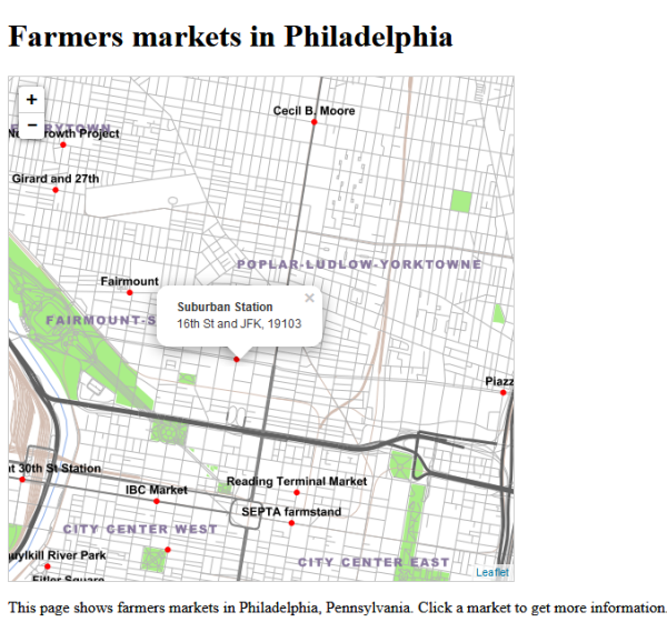
Figure 6.7 Final web page after completing the walkthrough
Troubleshooting
If you don't get the expected result at the end of the walkthrough, please verify the following:
- Make sure that you are connected to the Internet. In this course, we always reference Leaflet from a content delivery network (CDN) website rather than hosting it on our own server. All of the Leaflet logic is being pulled from the Internet in our case.
- Check that GeoServer is started. Note that you may need to stop GeoServer while making adjustments to your code, then start it when you have made your edits and want to preview your work.
- Make sure that you are opening the page in your browser via the http://localhost:8080/geog585/markets.html [165] URL and not as a local file, e.g. by double-clicking the .html file in the Windows File Explorer.
- Check that you have correctly inserted your AWS S3 bucket addres into the tile URL for the basemap as described above.
- Check that you have inserted the correct workspace and web service name in your WMS URL as described above.
- Make sure your code exactly matches the final code below other than the parts your personalized in the two previous steps.
Final code for the walkthrough
Below is the code used in this walkthrough from start to finish (but keep in mind that the URL for the basemap tiles needs to be adapted to refer to your S3 bucket). This should help you get some context of where each block should be placed. If you’re curious how the code would look in a different API, you can download an OpenLayers 3 example [166] here.
<!DOCTYPE html>
      <html>
        <head>
          <meta http-equiv="Content-Type" content="text/html; charset=utf-8">
            <title>Farmers markets in Philadelphia</title>
            <link rel="stylesheet" href="https://cdnjs.cloudflare.com/ajax/libs/leaflet/1.2.0/leaflet.css" type="text/css" crossorigin="">
            <script src="https://cdnjs.cloudflare.com/ajax/libs/leaflet/1.2.0/leaflet.js"></script>
            <script src="http://ajax.googleapis.com/ajax/libs/jquery/1.9.1/jquery.min.js"></script>
            <link rel="stylesheet" href="style.css" type="text/css">
            <script type="text/javascript">

            var map;

            function init() {
              // create map and set center and zoom level

              map = new L.map('mapid');
              map.setView([39.9526,-75.1652],13);

              // create tile layer and add it to map
              var tiles = L.tileLayer('https://<URL of your S3 bucket>/PhillyBasemap/{z}/{x}/{y}.png');
              tiles.addTo(map);

              // create wms layer
              var farmerMarkets = L.tileLayer.wms('http://localhost:8080/geoserver/geog585/wms', {
                layers: 'geog585:FarmersMarkets',
                format: 'image/png',
                transparent: true
              });

              farmerMarkets.addTo(map);

              // define event handler function for click events and register it

              function Identify(e)
              {
                // set parameters needed for GetFeatureInfo WMS request
                var sw = map.options.crs.project(map.getBounds().getSouthWest());
                var ne = map.options.crs.project(map.getBounds().getNorthEast());
                var BBOX = sw.x + "," + sw.y + "," + ne.x + "," + ne.y;
                var WIDTH = map.getSize().x;
                var HEIGHT = map.getSize().y;

                var X = Math.trunc(map.layerPointToContainerPoint(e.layerPoint).x);
                var Y = Math.trunc(map.layerPointToContainerPoint(e.layerPoint).y);

                // compose the URL for the request
                var URL = 'http://localhost:8080/geoserver/geog585/wms?SERVICE=WMS&VERSION=1.3.0&REQUEST=GetFeatureInfo&LAYERS=geog585:FarmersMarkets&QUERY_LAYERS=geog585:FarmersMarkets&BBOX='+BBOX+'&FEATURE_COUNT=1&HEIGHT='+HEIGHT+'&WIDTH='+WIDTH+'&INFO_FORMAT=application%2Fjson&TILED=false&CRS=EPSG%3A3857&I='+X+'&J='+Y;

                //send GetFeatureInfo as asynchronous HTTP request using jQuery $.ajax

                $.ajax({
                   url: URL,
                   dataType: "json",
                   type: "GET",
                   success: function(data)
                   {
                     if(data.features.length !== 0) {  // at least one feature returned in response
                       var returnedFeature = data.features[0]; // first feature from response

                       // Set up popup for clicked feature and open it
                       var popup = new L.Popup({
                         maxWidth: 300
                       });

                       popup.setContent("<b>" + returnedFeature.properties.NAME + "</b><br />" + returnedFeature.properties.ADDRESS);
                       popup.setLatLng(e.latlng);
                       map.openPopup(popup);
                    }
                  }
                 });
               }

               map.addEventListener('click', Identify);

             }

          </script>
        </head>
        <body onload="init()">
          <h1 id="title">Farmers markets in Philadelphia</h1>
          <div id="mapid">
          </div>
          <div id="docs">
              <p>This page shows farmers markets in Philadelphia, Pennsylvania. Click a market to get more information.</p>
          </div>
        </body>
      </html>
Lesson 6 assignment: Overlay your own data in Leaflet and examine real world use of a web mapping API
This week's assignment has two parts:
- The first piece of the assignment requires you to adapt the Lesson 6 walkthrough to your own data. Recall that in the Lesson 4 assignment, you served a WMS using some of your term project data. For this week's assignment, overlay this WMS on a tiled map using Leaflet. Get the popups working on the WMS as well.
The tiled map can either be the map you made in the Lesson 5 assignment, or it can be a third party hosted set of OpenStreetMap tiles.
This task will require just some minor adaptation of the walkthrough code.
The deliverables for this part of the project are A) your HTML source code file, B) a screenshot of the two maps overlayed with a popup displayed (just like the graphics in the walkthrough), and C) a short (200 - 300 word) write-up reflecting on how this part of the assignment went for you, what problems you encountered, and insights you gained from it.
- Read this GIS Stack Exchange post: How do various JavaScript mapping libraries compare? [145] Then write a short review of the bikeshare web map at https://bikesharemap.com/ [168]. Examine the source code (use "View Page Source" in your browser) and then submit an approximately 300 - 500 word evaluation describing:
- Which web mapping API was used?
- Which services/layers are brought into this map?
- What principal features/classes of the web mapping API were used? Include links to the API reference documentation for these classes.
- What is one coding technique you learned by looking at the source code of this map?
- What could be improved in this web map implementation in terms of code or additional interactive elements?
Zip these deliverables into a single folder and place them in the Lesson 6 assignment drop box on Canvas.
Lesson 7: Drawing vector layers on the client side
The links below provide an outline of the material for this lesson. Be sure to carefully read through the entire lesson before returning to Canvas to submit your assignments.
Note: You can print the entire lesson by clicking on the "Print" link above.
Overview
Note: Currently, this lesson teaches the Leaflet API. If you are looking for the previous materials on OpenLayers, see the Lesson 7 archive page [169].
Last week, you used a server-drawn image from a WMS to display your business layer (the farmers markets). This week, you'll learn about an alternative way to display your business layers on the map; namely, sending the raw data to the client (such as a web browser) to be drawn. This is a common technique in many web maps that can provide for much interactivity and potentially faster performance if used appropriately. You may have even been exposed to this practice when you reviewed a web map for your assignment last week.
This lesson describes two common formats used for sending vector GIS data to the browser (KML and GeoJSON) and shows how you can add these types of layers in Leaflet.
Objectives
- Describe benefits and challenges of drawing thematic vector map layers on the client.
- Choose between KML, GeoJSON, and other formats for drawing vector data on the client.
- Understand how vector layers can be symbolized on the fly to provide a more interactive web map experience.
- Draw thematic vector layers in a web map using Leaflet and change the symbolization in response to map events.
Checklist
- Read the Lesson 7 materials on this page.
- Complete the walkthrough.
- Complete the Lesson 7 assignment.
Benefits and challenges of drawing vector layers on the client side
Up to this point, your web maps have displayed images obtained from the server: either through pre-drawn tiles or dynamically-drawn WMS maps. An alternative approach is to send some text to the client containing the coordinates and attributes of features, then allow the client to draw the layer. This approach can improve the speed and interactivity of your web map when used wisely.
You may be asking, "How does a client like a web browser know how to draw GIS data?" Although web browsers don't "know" anything about GIS, they indeed have the ability to draw vector graphics, which is just the simple process of connecting screen coordinates with a symbol. Web mapping APIs can read a series of coordinates provided in a GeoJSON file, or a KML file, to give a few examples, and convert these into screen coordinates to be drawn by the browser.
Advantages of drawing vectors on the client
Speed and interactivity are two principal advantages of drawing vector features on the client rather than the server. Once your web browser has read the vector data from the server, users of the web map can interact with the data in a lightning fast manner. Let's suppose I have a web map of the United States with all the NFL football teams displayed on it. The basemap is coming from an OpenStreetMap tiled layer. The football teams are coming from a GeoJSON file. When the map loads, all the GeoJSON for the teams is read by my web browser. This includes all geographic coordinates and the attribute information for each team. Now I can click on any team and see its information without making another request to the server. Contrast this with the farmers markets mashup from the previous lesson, which required a WMS GetFeatureInfo query to the server (and the associated wait time) any time you clicked a market.
Let's suppose I want to highlight a map symbol whenever a user hovers over it, thereby providing a visual cue that someone can click the symbol. A web browser can change the symbol styling quickly enough that this effect works. In contrast, if a round trip to the server were required on every hover event, my app (and possibly my server) could easily grind to a standstill.
Challenges with drawing vectors on the client
Not all use cases are appropriate for drawing vectors on the client side. If you're displaying hundreds of features at a time, or some complex polygons with many vertices, you're probably better off asking the server to draw the map and send it to you. Browsers can get weighed down to a crawl if handed too many vector graphics to draw at once. Sending a lot of complex graphics also results in more network traffic, as all the coordinates must be downloaded by the client.
To keep performance crisp, it's a good idea to generalize the layers that you draw on the client as much as possible, at least at the smallest map scales. For example, when displaying the United States at the nationwide level, you should not be using a file that contains every tiny coastal island in the state of Maine. You might switch to loading a more detailed file when the user zooms in past a particular scale.
Labeling can also be a challenge with browser-drawn graphics. Although web browsers can draw text on the screen at a given coordinate, they have no label placement algorithms like the ones employed by GeoServer, QGIS or TileMill. Your labels will likely overlap each other. You are better off allowing the user to discover the label through interactivity, displaying the label in a popup or HTML DIV when someone clicks a feature.
Finally, the symbol choices offered by web browsers are relatively elementary. You can always instruct the browser to draw a graphic, such as an SVG file, but you won't be able to get some of the complex lines and fills available in programs like QGIS or ArcGIS. Of course, if your client happens to be a desktop application such as QGIS, you don't have to worry as much about available symbol choices.
How to draw vectors on the client
Web mapping APIs typically provide classes for drawing vector layers with the browser; however, these go by different names with each API. For a few simple standalone vectors, you will often see a "marker" class. For more complex layers, you may see something like FeatureGroup (Leaflet) or FeatureLayer (Esri). OpenLayers has a Layer.Markers class and a Layer.Vector class for these respective purposes.
Desktop programs such as QGIS can view KML, GeoJSON, GML (described in Lesson 8), and various other text-based vector data formats.
Approaches for retrieving data from the server
When you define a vector layer, you need to specify the approach that your client will take for retrieving the data from the server. Remember that your client is not requesting map images from the server, but it does need to retrieve the coordinates of the vectors and any associated attribute information. Some popular approaches include:
- Retrieve all the data at the time the layer is loaded. In Leaflet, this is the default behavior. It requires an initial performance hit, but it makes your application responsive by ensuring that it never has to go back to the server to make another request. This approach is inappropriate for very large amounts of data.
- Retrieve only the data within the current map view. When the map view changes, make a new request. Although OpenLayers offers this approach through its "bbox" loading strategy [170], I am not aware of this functionality being available in Leaflet out of the box (please correct me if you know otherwise). It works well when there's too much data in the dataset to download at once, but it can make your map seem clunky if people zoom and pan very quickly. Sometimes, logic is incorporated to retain features already requested (for example, in the case of a small map pan where the new map view includes some features that were previously downloaded).
- Retrieve only some of the vector features from the dataset based on a filter or query condition. Leaflet offers a filter option when you create a GeoJSON layer. This can narrow down the data requested, allowing you to get the effect of the first approach (retrieve all data) without downloading the entire dataset.
- Retrieve vectors in uniformly sized chunks, or "vector tiles" as you learned about in Lesson 5. This is only possible if the server administrator has pregenerated a set of tiles. Various plugins [171]are available for consuming vector tiles via Leaflet. OpenLayers versions 3 and above have a VectorTile [172] layer class designed for this.
You may see other variations on the above approaches, including the re-loading of layers at fixed intervals to represent an ever-changing phenomenon, such as the position of a fleet of ships.
Working with vector KML
KML (Keyhole Markup Language) is a popular format for vector GIS features due to its association with Google Earth and Google Maps. KML is just XML formatted according to an open specification, previously maintained by Google, but now enshrined in an OGC standard. Although KML can define the placement of raster layers, we will focus on vector KML in this lesson.
The key XML tag behind KML is the placemark. This defines a geographic feature, a symbol, and extra information that can appear in a popup. You can see some placemarks if you save the example KML file [173] and open it in a text editor. This isn't the cleanest file, but it will do for the purposes of seeing a placemark:
<Placemark>
	   <name>Sundial, Plymouth, Devon, UK</name>
               <description><![CDATA[The gnonom is 27 feet high, the pool has 21 feet diameter.  It was designed by architect Carole Vincent from Boscastle in Cornwall and was unveiled by Her Majesty the Queen on Friday, July 22nd, 1988 at a cost of cost £70,000. The sundial runs one hour and seventeen minutes behind local clocks.
	<img src="http://www.photoready.co.uk/people-life/images/sundial-fountain.jpg">
	Image source:<a href="www.photoready.co.uk</a>]]>
           </description>
	   <LookAt>
	      <longitude>-4.142398271107962</longitude>
	      <latitude>50.37145390235462</latitude>
	      <altitude>0</altitude>
	      <range>63.33410419881957</range>
	      <tilt>0</tilt>
	      <heading>-0.0001034131369701296</heading>
	   </LookAt>
	   <styleUrl>#msn_sunny_copy69</styleUrl>
	   <Point>
	      <coordinates>-4.142446411782089,50.37160252809223,0</coordinates>
	   </Point>
	</Placemark>
This particular placemark has a single coordinate, contained in the Point tag. For polylines and polygons, the LineString and Polygon tags are used, respectively, although these do not appear in the above example.
Notice that the Description tag can contain HTML, which gives you more control over formatting popups. The full KML file is much longer than the snippet above, as it contains many points and descriptions.
Leaflet doesn't offer a way to read KML directly. This is an area where OpenLayers holds an advantage. However, Mapbox has produced a free Leaflet plugin called Omnivore that makes it fairly simple to read in vector file types, including KML. First, you need to put a reference to Omnivore in a script tag at the top of your page. You could reference it from a CDN like this:
<script src="https://cdnjs.cloudflare.com/ajax/libs/leaflet-omnivore/0.3.4/leaflet-omnivore.js"></script>
Then you can reference the KML in a layer, like this:
var runLayer = omnivore.kml('sundials.kml')
  .on('ready', function() {
    map.fitBounds(runLayer.getBounds());

    runLayer.eachLayer(function(layer) {
      layer.bindPopup(layer.feature.properties.description);
    });
  })
  .addTo(map);
One thing to be aware of is that Omnivore converts the KML to the GeoJSON format before displaying it; (see the next section of the lesson for more info on GeoJSON). Thus, your map may not be able to show all the styling that was originally defined in the KML. If your KML contains some kind of custom picture symbol for the points, you'll need to write Leaflet code to apply that picture to the markers. Notice, however, that the above code does bring in the KML description and applies that text in a popup. This is accomplished using the bindPopup method on the layer.
Again, don't worry about memorizing all the syntax. In most scenarios, you should just be able to tweak the above example to connect to your own KML.
Working with GeoJSON
GeoJSON is a widely-used data format for displaying vectors in web maps. It is based on JavaScript object notation, a simple and minimalist format for expressing data structures using syntax from JavaScript. In GeoJSON, a vector feature and its attributes are represented as a JavaScript object, allowing for easy parsing of the geometry and fields.
GeoJSON is less bulky than XML-based structures such as KML; however, GeoJSON does not always contain styling information like KML does. You must define the styling on the client, which in your case means writing JavaScript code or taking the Leaflet's default styling. This is covered in the next section of the lesson.
GeoJSON's simplicity and loading speed have made it popular, perhaps even trendy, among developers in the FOSS world. For example, in a tongue-in-cheek Internet poll, GIS practitioners recently voted "The answer is always GeoJSON" as the most likely attribute to define a 'GeoHipster' [174].
Here's what a piece of GeoJSON looks like. GeoJSON vectors are commonly bundled into a unit called a FeatureCollection. The FeatureCollection below holds just one feature (the state of Montana) but could hold other features. The bulk of the GeoJSON below contains the vertices that define the state outline, but you should also notice a few attributes, such as "fips" and "name":
{"type":"FeatureCollection","features":[{"type":"Feature","id":"USA-MT","properties":{"fips":"30","name":"Montana"},"geometry":{"type":"Polygon","coordinates":[[[-104.047534,49.000239],[-104.042057,47.861036],[-104.047534,45.944106],[-104.042057,44.996596],[-104.058488,44.996596],[-105.91517,45.002073],[-109.080842,45.002073],[-111.05254,45.002073],[-111.047063,44.476286],[-111.227803,44.580348],[-111.386634,44.75561],[-111.616665,44.547487],[-111.819312,44.509148],[-111.868605,44.563917],[-112.104113,44.520102],[-112.241036,44.569394],[-112.471068,44.481763],[-112.783254,44.48724],[-112.887315,44.394132],[-113.002331,44.448902],[-113.133778,44.772041],[-113.341901,44.782995],[-113.456917,44.865149],[-113.45144,45.056842],[-113.571933,45.128042],[-113.736241,45.330689],[-113.834826,45.522382],[-113.807441,45.604536],[-113.98818,45.703121],[-114.086765,45.593582],[-114.333228,45.456659],[-114.546828,45.560721],[-114.497536,45.670259],[-114.568736,45.774321],[-114.387997,45.88386],[-114.492059,46.037214],[-114.464674,46.272723],[-114.322274,46.645155],[-114.612552,46.639678],[-114.623506,46.705401],[-114.886399,46.809463],[-114.930214,46.919002],[-115.302646,47.187372],[-115.324554,47.258572],[-115.527201,47.302388],[-115.718894,47.42288],[-115.724371,47.696727],[-116.04751,47.976051],[-116.04751,49.000239],[-111.50165,48.994762],[-109.453274,49.000239],[-104.047534,49.000239]]]}}]}
In the GeoJSON above, notice the use of several JavaScript objects embedded within one another. At the lowest level, you have a Polygon object. The Polygon object is contained within a Feature object. The feature is part of a FeatureCollection object. The GeoJSON specification [62] (originally published in 2008 but replaced by a new specification in 2016) gives precise details about how these objects are to be structured. It's important to be familiar with these structures, although you will rarely have to read or write them directly. You will typically use convenience classes or converter programs that have been developed to simplify the experience of working with GeoJSON.
You can use GeoJSON within your main JavaScript code file, but, to keep your things looking simple, it's most common to maintain the GeoJSON in its own separate file. You then reference this file from the appropriate place in your code. With Leaflet you have to define the GeoJSON as a JavaScript variable (seen here) [175] using syntax such as
var <yourVariableName> = <yourGeoJSON>;
You would save this text in a file with a .js extension. For example, I could create a file titled myfeatures.js containing something like the following:
var myGardenJson = {"type":"FeatureCollection","features":[{"type":"Feature","id":"USA-MT","properties":{"fips":"30","name":"Montana"},"geometry":{"type":"Polygon","coordinates":[[[-104.047534,49.000239], . . . ]]}}]};
Then at the top of my HTML page, I need to put a reference to this file:
<script src="myfeatures.js"></script>
This allows me to reference the variable myGardenJson within my JavaScript code. Making a GeoJSON layer in Leaflet then becomes very simple:
var geojsonLayer = L.geoJSON(myGardenJson);
geojsonLayer.addTo(map);
It is important to note that L.geoJSON(…) expects all coordinates in the GeoJSON file to be WGS84 coordinates. That is why all GeoJSON files used in this lesson and Lesson 8 will use EPSG:4326. If instead you want to directly work with a GeoJSON file that uses a different projection (so without first reprojecting it to EPSG:4326), you can use the Proj4js [176] Javascript library together with the Proj4Leaflet [177] extension to enable support for coordinate reference systems not built into Leaflet. To do so, you would first have to add the lines to load the respective Javascript libraries at the beginning of the html file
<script src="https://cdnjs.cloudflare.com/ajax/libs/proj4js/2.4.3/proj4.js"></script>
<script src="https://cdnjs.cloudflare.com/ajax/libs/proj4leaflet/1.0.1/proj4leaflet.min.js"></script>
and then create the layer with
var geojsonLayer = L.Proj.geoJson(myGardenJson);
to have the code read what projection the GeoJSON file is in and then reproject the data accordingly on the fly. Leaflet, by the way, internally uses pixel coordinates for all data, so it understands locations with respect to the coordinate system of the map pane. That means that there is always a transformation process involved when loading vector data, independent of what projection the data comes in.
You can save any vector layer in QGIS as GeoJSON, and most web mapping APIs offer easy-to-use classes for GeoJSON as a vector display format. In the proprietary software realm, Esri has dragged its feet on GeoJSON support, offering its own JSON-based geometry formats [178] as part of the GeoServices REST Specification and the ArcGIS REST API; however, Esri has informally shared an open source JavaScript library [179]to convert between the two formats, which is now deprecated and replaced by their Terraformer tool [180].
The GeoJSON specification is not an OGC specification. At the time of this writing, OGC conspicuously lacks a JSON-based specification for defining vector GIS objects (OGC publishes the XML-based GML specification for vectors). This lack of an OGC-endorsed JSON specification played a role in the FOSS community's 2013 debate about whether the OGC should adopt the Esri-generated GeoServices REST Specification. The specification would have given OGC a JSON-based GIS data format, but some were wary of the format's association with a proprietary software company. The geoMusings "OGC Abandons the Web" [181] blog post gives one FOSS geo-developer's opinion on the episode (read the comments, too).
Symbolizing vector layers in Leaflet
When you bring in vector datasets to be drawn by the browser, you may need to do some work to define the symbol that will draw the feature. With data formats like GeoJSON that don't contain any styling information, you don't get ready-made styling like you would get if you just requested an image from the server. If you don't define a symbol for your graphics, you'll probably see your API's default symbol.
In Leaflet, it's common to define styles within functions. This makes them easy to re-use. Here's an example of how you could set up a style and apply it to a GeoJSON layer. This example shows urban gardens as polygons:
// Set up style for garden polygons
function gardenStyle(feature) {
  return {
    fillColor: "#FF00FF",
    fillOpacity: 1,
    color: '#B04173',
    weight: 4,
  };
}

// Create layer and add it to the map
var gardenLayer = L.geoJSON(myGardenJson,{
  style:gardenStyle
});

gardenLayer.addTo(map);
Notice that the properties include fill color, fill opacity (which controls transparency), stroke color, and stroke weight. The colors are defined using hex notation [182]. In this case, the symbol is a magenta fill with a purple outline (Sorry! I wanted it to stand out...). When writing your own code, use an online color picker [183] to get the hex values of the colors you want.
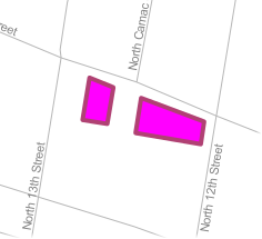
You can see a list of Leaflet's vector styling properties by reading the Path options [184] documentation. You should be able to accomplish most of what you want to do using working examples and a little bit of experimentation.
The advantage of drawing vector layers in the browser is that you can quickly change the styling in response to certain events. For example, you can change the color of a single symbol when a user clicks it. Using Leaflet, you can define various styles and connect them to map events.
The code below demonstrates how a style map could be used to "highlight" a garden feature when it's clicked. The selected garden would change to a blue fill:
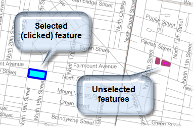
Don't worry about running this code right now, because you'll use some nearly identical code in the lesson walkthrough in a working example. Just pay attention to the code patterns and what is happening in each line.
First, create functions to define the unselected and selected styles:
// Set up styles for garden polygons
// Magenta symbol for gardens
function gardenStyle(feature) {
  return {
    fillColor: "#FF00FF",
    fillOpacity: 1,
    color: '#B04173',
    weight: 4,
  };
}

// Blue symbol for selected gardens
function gardenSelectedStyle(feature) {
  return {
    fillColor: "#00FFFB",
    fillOpacity: 1,
    color: '#0000FF',
    weight: 4
  };
}
Then create the GeoJSON layer and add functions to listen for click events on the GeoJSON features and the map itself. The code below contains a variable named selection, which holds the currently selected feature. The expression if (selection) checks to see if there is any selected feature. The expression e.target means "the feature that just got clicked". Notice how the resetStyle method can set a layer's style back to its original form, and the setStyle method can change a feature's style to something new.
var selection;

// define function to handle click events on garden features
function gardenOnEachFeature(feature, layer){
  layer.on({
    click: function(e) {
      if (selection) {
        gardenLayer.resetStyle(selection);
      }

      e.target.setStyle(gardenSelectedStyle());
      selection = e.target;

      L.DomEvent.stopPropagation(e); // stop click event from being propagated down to other elements
    }
  });
}


// Create layer and add it to the map
var gardenLayer = L.geoJSON(myGardenJson,{
  style:gardenStyle,
  onEachFeature: gardenOnEachFeature
});

gardenLayer.addTo(map);


// define and register event handler for click events to unselect features when clicked anywhere else on the map
map.addEventListener('click', function(e) {
  if (selection) {
     gardenLayer.resetStyle(selection);

     selection = null;
  }
});
A map user should now be able to click any garden and see it highlighted in blue. When the user clicks off the garden, it goes back to its original magenta symbol.
To summarize this part of the lesson, vector layers drawn by the browser require a little more work on the developer's part, because the developer must define the symbols. However, with that work comes a variety of options for interactivity that would not be possible with rasterized image tiles or layers drawn by the server. Although the resymbolize-on-click functionality seems rudimentary, think about the difficulty (if not outright futility) of getting this type of effect with a WMS or rasterized tile layer.
This section of the lesson has discussed uniform symbols for each feature in the layer (except for the occasional selected feature); however, Leaflet allows you to go further by defining style classifications based on attribute values. This opens the door for choropleth maps, proportional symbols, and so forth. Some of these techniques will be covered in Lesson 8.
Allowing developers untrained in cartographic principles to select map symbols may present some challenges of its own. It may be a good idea to have the developer consult with a cartographer in order to determine the most appropriate widths, colors, and fills for the vector symbols.
Walkthrough: Adding interactive GeoJSON layers in Leaflet
This walkthrough builds on some of the previous sections of the lesson to show how you can add interactive GeoJSON layers to your web map using Leaflet. You will build a map containing your Philadelphia basemap tiles and two GeoJSON layers on top representing urban gardens and food pantries (i.e., food banks). A user can click one of the gardens or food pantries to see the name of the feature below the map (as an alternative to using popups). The clicked feature changes color while it is selected. Hopefully, you can think of many ways to apply these pieces of functionality to the web map you're building for your term project.
Note that this is a sample dataset culled from OpenStreetMap and is not a comprehensive list of these features in Philadelphia. If you know of any other gardens or food pantries, please add them in OpenStreetMap (more about this in Chapter 9)!
Downloading the data
Before continuing, download and unzip the data for this project [185]. Copy its contents into your Jetty home folder, which should have a path such as
c:\Users\{username}\GeoServer 2.x.x\webapps\geog585\
This is the same folder where you saved your Lesson 6 walkthrough and where your local stylesheet style.css (required for this exercise) is located.
This folder contains two JavaScript files containing GeoJSON data. gardens.js holds a gardensData variable with polygon GeoJSON and pantries.js holds a pantriesData variable with point GeoJSON.
There are also two SVG (scalable vector graphics) files that will be used for symbolizing the food pantries. The yellow symbol will be for the unselected features and the blue symbol for the selected features.
There are a couple of ways that you could get this kind of data for your own applications.
- QGIS can save any vector layer as GeoJSON format.
- ogr2ogr in the GDAL library can convert shapefiles and other types to GeoJSON
In both cases you would need to either save the data as a JS file and define the GeoJSON as a variable (the approach we took here), or use an extension like Leaflet AJAX to read the data directly out of the file (beyond the scope of this course).
To get icons, all the icons available in QGIS are available on your machine in a folder named something like:
C:\Program Files\QGIS <name of your version>\apps\qgis\svg
I used the open source program Inkscape to change the color of the icon.
Setting up the HTML file
Before diving into the JavaScript code, create an empty text file and insert the following code. Then save it as lesson7.html next to all the other files you just downloaded and copied into your home folder.
<!DOCTYPE html>
  <html>
    <head>
      <meta http-equiv="Content-Type" content="text/html; charset=utf-8">
      <title>Food resources: Community gardens and food pantries</title>
      <link rel="stylesheet" href="https://cdnjs.cloudflare.com/ajax/libs/leaflet/1.2.0/leaflet.css" type="text/css" crossorigin="">
      <script src="https://cdnjs.cloudflare.com/ajax/libs/leaflet/1.2.0/leaflet.js" crossorigin=""></script>
      <script src="gardens.js"></script>
      <script src="pantries.js"></script>
      <link rel="stylesheet" href="style.css" type="text/css">

        <script type="text/javascript">

        . . .

        </script>
    </head>
      <body onload="init()">
        <h1 id="title">Food resources: Community gardens and food pantries</h1>

        <div id="mapid"></div>
        <div id="summaryLabel">
            <p>Click a garden or food pantry on the map to get more information.</p>
        </div>
      </body>
  </html>
If you open this, you should see a blank map frame surrounded by an HTML title and descriptive text. In the script and link tags, notice that we are loading in Leaflet code and stylesheets, as well as the gardens and pantries.js files.
Now let's add the Leaflet JavaScript code that creates the map and layers.
Writing the JavaScript
- Find the script tag for your JavaScript code and replace the . . . with the following lines so that you have:
var map;

function init() {
  // create map and set center and zoom level
  map = new L.map('mapid');
  map.setView([39.960,-75.210],14);

  // create and add the tile layer
  var tiles = L.tileLayer('https://<URL of your S3 bucket>/PhillyBasemap/{z}/{x}/{y}.png');
  tiles.addTo(map);

 . . .

}
The above code creates a global variable for the map and then defines the initialization function that will run when the page loads. This init() function will contain most of our JavaScript code.
The map view is set zoomed in to West Philadelphia so we can get a detailed look at food resources at a neighborhood level.
The Philadelphia basemap tiles are also added here. You must modify the URL in the code above to point at your own tiles as you had to do in the Lesson 6 walkthrough. Again the URL should look similar to this with the first part being the URL of your S3 bucket:https://geog585-somestring.s3.someregion.amazonaws.com/PhillyBasemap/{z}/{x}/{y}.png - Now we'll set up some variables for use in this init() function. Replace the . . . in the code above with the following:
var gardenLayer;
var pantryLayer;

var selection;
var selectedLayer;

. . .
Nothing is happening with these yet, but it's important that you understand their future purpose in the code:
- gardenLayer and pantryLayer will eventually be Leaflet layers that reference the GeoJSON.
- selection will reference the currently selected feature. If no feature is selected, the value of this variable will be set to null.
- selectedLayer will reference the layer that was most recently selected.
- Now we'll set up the style we'll eventually use on the garden layer. Replace the . . . in the code above with the following:
// define the styles for the garden layer (unselected and selected)
function gardenStyle(feature) {
  return {
    fillColor: "#FF00FF",
    fillOpacity: 1,
    color: '#B04173',
  };
}

function gardenSelectedStyle(feature) {
  return {
    fillColor: "#00FFFB",
    color: '#0000FF',
    fillOpacity: 1
  };
}

. . .
This is nearly identical to the code in the previous section of the lesson, so I won't explain it in detail. It just defines two different symbols for the gardens layer (a default symbol and a selected symbol).
- Now let's add a function that will tell each garden feature how to behave when it is clicked. Replace the . . . in the code above with the following:
// handle click events on garden features
function gardenOnEachFeature(feature, layer){
  layer.on({
    click: function(e) {
      if (selection) {
        resetStyles();
      }

      e.target.setStyle(gardenSelectedStyle());
      selection = e.target;
      selectedLayer = gardenLayer;

      // Insert some HTML with the feature name
      buildSummaryLabel(feature);

      L.DomEvent.stopPropagation(e); // stop click event from being propagated further
    }
  });
}

. . .
There's a lot going on here, so we'll take this a piece at a time. One of the most useful things about Leaflet is its ability to define a function for each feature stating how that feature should behave in response to certain events. In the function above, we're telling each garden feature to listen for a click event. If a garden gets clicked, a function will run with an event argument (represented by the variable e) that will help us work with the clicked feature. This code is called event handler code, because it handles the situation where a click event occurs.
In the case above, if a feature gets clicked, we take any existing feature that might be highlighted and set its style back to the default. This is accomplished in the function resetStyles() whose code we are going to add later on.
Then we take the clicked feature (e.target) and style it with the special style we set up for selected features. We also update the selection and selectedLayer variables to reference our newly clicked feature.
Finally, we build some HTML to put in the descriptive layer below the map. This code will be found in a function called buildSummaryLabel(), which we will add a little later on.
Note that a call to L.DomEvent.stopPropogation() is needed so that if someone clicks a feature, only the feature click event handler code runs, and not the map click event handler code.
- Now we've got everything we need to add the garden layer to the map. Replace the . . . in the code above with the following:
// add the gardens GeoJSON layer using the gardensData variable from gardens.js
var gardenLayer = new L.geoJSON(gardensData,{
  style: gardenStyle,
  onEachFeature: gardenOnEachFeature
});

gardenLayer.addTo(map);

. . .
Note how the above code references the gardensData variable contained in gardens.js. If we didn't have a script tag referencing gardens.js at the top of our page, the variable gardensData would be unrecognized. By using gardenStyle for the style property, we are making sure that the layer will be styled according to our previous definition. Similarly, by using the gardenOnEachFeature function defined above for the onEachFeature property, we achieve that each feature from the layer will have the click event handler function defined in gardenOnEachFeature attached.
- Now we're going to repeat the whole process with the pantries layer. Replace the . . . in the code above with the following:
// create icons for pantries (selected and unselected)
var pantriesIcon = L.icon({
  iconUrl: 'pantries.svg',
  iconSize: [20,20]
});

var selectedPantriesIcon = L.icon({
  iconUrl: 'pantries_selected.svg',
  iconSize: [20,20]
});

// handle click events on pantry features
function pantriesOnEachFeature(feature, layer){
  layer.on({
    click: function(e) {
      if (selection) {
        resetStyles();
      }

      e.target.setIcon(selectedPantriesIcon);
      selection = e.target;
      selectedLayer = pantryLayer;

      // Insert some HTML with the feature name
      buildSummaryLabel(feature);

      L.DomEvent.stopPropagation(e); // stop click event from being propagated further
    }
  });
}


// add the pantries GeoJSON layer using the pantriesData variable from pantries.js
pantryLayer = new L.geoJSON(pantriesData,{
  pointToLayer: function (feature, latlng) {
    return L.marker(latlng, {icon: pantriesIcon});
  },
  onEachFeature: pantriesOnEachFeature
  }
);

pantryLayer.addTo(map);

. . .
The only fundamental difference between this and the gardens code is the way that the style is defined for a point using an SVG icon. Notice how when the Leaflet layer is created, the pointToLayer function must be defined stating where and how to place each Leaflet marker.
- Now that all the layers are added, let's switch our focus to the map. We have to handle the case where someone clicks on the map but doesn't click on a feature. In that situation, everything should become unselected. Replace the . . . in the code above with the following:
// handle clicks on the map that didn't hit a feature
map.addEventListener('click', function(e) {
  if (selection) {
    resetStyles();
    selection = null;
    document.getElementById('summaryLabel').innerHTML = '<p>Click a garden or food pantry on the map to get more information.</p>';
  }
});

. . .
There are several ways that event handlers can be added in Leaflet. The code above uses the addEventListener method. Notice how in the above code the label below the map is also reset with the message "Click a garden or food pantry on the map to get more information."
- Now we'll add some of the functions that were used in the layer event handler code above. The first one looks to see which layer was previously selected and sets the selected feature's symbol back to the default. Replace the . . . in the code above with the following:
// function to set the old selected feature back to its original symbol. Used when the map or a feature is clicked.
function resetStyles(){
  if (selectedLayer === pantryLayer) selection.setIcon(pantriesIcon);
  else if (selectedLayer === gardenLayer) selectedLayer.resetStyle(selection);
}

. . .
Separate lines of code are needed above for the pantries and gardens layers because points represented by icons and polygons have different styling syntaxes in Leaflet.
- Finally we need the function to build the HTML string for the summary label that goes below the map. Replace the . . . in the code above with the following:
// function to build the HTML for the summary label using the selected feature's "name" property
function buildSummaryLabel(currentFeature){
  var featureName = currentFeature.properties.name || "Unnamed feature";
  document.getElementById('summaryLabel').innerHTML = '<p style="font-size:18px"><b>' + featureName + '</b></p>';
}
The above function brings in the currently selected feature and reads its "name" attribute. It then gets the HTML element with the ID of "summaryLabel" and sets its innerHTML to a carefully constructed string of HTML into which the name (represented by the variable featureName) is inserted. Note that if our gardens and pantries layers had different attribute field names (such as "PANTRYNAME" and "GARDENNAME" then we would need to add more code above to handle those cases.
- Run your page, and click some of the garden and pantry features. When you click a feature, it should turn blue, and the feature name should display below the map. When you click away from a feature (or click a different feature), the feature should return to its original color, and the feature name should be removed (or updated if you clicked a different feature).
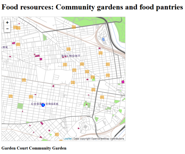 Figure 7.4
Final code for the walkthrough
If your page does not work, carefully compare your code to the full code below to make sure you have inserted everything in the right place. Also:
- Verify that you are connected to the Internet when you run the page, so that you can retrieve the Leaflet code from the CDN.
- Make sure that you have inserted the URL for your S3 bucket where the code refers to the basemap tile layer.
- Make sure that GeoServer is started (because you are running the page through its Jetty web servlet) and that you are referencing the page through a URL similar to the following: http://localhost:8080/geog585/lesson7.html [186].
An OpenLayers 3 version of the walkthrough code [187] is available for the curious. Note that the GeoJSON files must be adjusted for this version of the walkthrough to function. It must be pure GeoJSON and not contain any declared variables or JavaScript code.
<!DOCTYPE html>
  <html>
    <head>
      <meta http-equiv="Content-Type" content="text/html; charset=utf-8">
      <title>Food resources: Community gardens and food pantries</title>
      <link rel="stylesheet" href="https://cdnjs.cloudflare.com/ajax/libs/leaflet/1.2.0/leaflet.css" type="text/css" crossorigin="">
      <script src="https://cdnjs.cloudflare.com/ajax/libs/leaflet/1.2.0/leaflet.js" crossorigin=""></script>
      <script src="gardens.js"></script>
      <script src="pantries.js"></script>
      <link rel="stylesheet" href="style.css" type="text/css">

        <script type="text/javascript">
          var map;

          function init() {
          // create map and set center and zoom level
          map = new L.map('mapid');
          map.setView([39.960,-75.210],14);

          // create and add the tile layer
          var tiles = L.tileLayer('https://<URL of your S3 bucket>/PhillyBasemap/{z}/{x}/{y}.png');
          tiles.addTo(map);

          var gardenLayer;
          var pantryLayer;

          var selection;
          var selectedLayer;

          // define the styles for the garden layer (unselected and selected)
          function gardenStyle(feature) {
            return {
               fillColor: "#FF00FF",
               fillOpacity: 1,
               color: '#B04173',
            };
          }

          function gardenSelectedStyle(feature) {
             return {
               fillColor: "#00FFFB",
               color: '#0000FF',
               fillOpacity: 1
            };
          }

          // handle click events on garden features
          function gardenOnEachFeature(feature, layer){
            layer.on({
              click: function(e) {
                  if (selection) {
                    resetStyles();
                  }

                  e.target.setStyle(gardenSelectedStyle());
                  selection = e.target;
                  selectedLayer = gardenLayer;

                  // Insert some HTML with the feature name
                  buildSummaryLabel(feature);

                  L.DomEvent.stopPropagation(e); // stop click event from being propagated further
                }
            });
          }

                // add the gardens GeoJSON layer using the gardensData variable from gardens.js
                var gardenLayer = new L.geoJSON(gardensData,{
                  style: gardenStyle,
                  onEachFeature: gardenOnEachFeature
                });

                gardenLayer.addTo(map);


          // create icons for pantries (selected and unselected)
          var pantriesIcon = L.icon({
            iconUrl: 'pantries.svg',
            iconSize: [20,20]
          });

          var selectedPantriesIcon = L.icon({
            iconUrl: 'pantries_selected.svg',
            iconSize: [20,20]
          });

          // handle click events on pantry features
          function pantriesOnEachFeature(feature, layer){
            layer.on({
              click: function(e) {
                  if (selection) {
                    resetStyles();
                  }
                  e.target.setIcon(selectedPantriesIcon);
                  selection = e.target;
                  selectedLayer = pantryLayer;

                  // Insert some HTML with the feature name
                  buildSummaryLabel(feature);

                  L.DomEvent.stopPropagation(e); // stop click event from being propagated further
                }
            });
          }


          // add the pantries GeoJSON layer using the pantriesData variable from pantries.js
                pantryLayer = new L.geoJSON(pantriesData,{
                     pointToLayer: function (feature, latlng) {
                      return L.marker(latlng, {icon: pantriesIcon});
                     },
                     onEachFeature: pantriesOnEachFeature
                   }
                );

               pantryLayer.addTo(map);


          // handle clicks on the map that didn't hit a feature
          map.addEventListener('click', function(e) {
            if (selection) {
              resetStyles();
              selection = null;
              document.getElementById('summaryLabel').innerHTML = '<p>Click a garden or food pantry on the map to get more information.</p>';
            }
          });

          // function to set the old selected feature back to its original symbol. Used when the map or a feature is clicked.
          function resetStyles(){
            if (selectedLayer === pantryLayer) selection.setIcon(pantriesIcon);
            else if (selectedLayer === gardenLayer) selectedLayer.resetStyle(selection);
          }

          // function to build the HTML for the summary label using the selected feature's "name" property
          function buildSummaryLabel(currentFeature){
            var featureName = currentFeature.properties.name || "Unnamed feature";
            document.getElementById('summaryLabel').innerHTML = '<p style="font-size:18px"><b>' + featureName + '</b></p>';
          }

        }

        </script>
      </head>
      <body onload="init()">
        <h1 id="title">Food resources: Community gardens and food pantries</h1>

        <div id="mapid"></div>
        <div id="summaryLabel">
            <p>Click a garden or food pantry on the map to get more information.</p>
        </div>
      </body>
    </html>
Lesson 7 assignment: Make your own mashup with a vector layer drawn in the browser
In this week's assignment, you'll make a mashup consisting of a vector layer drawn by the browser on top of your own tiled basemap. To achieve this, you need to adapt the walkthrough techniques and code to your own data. Follow the instructions below to prepare this assignment:
- Examine your term project's tiled basemap. This could either be the one you created in the Lesson 5 assignment or a tiled map from OpenStreetMap that you want to use.
- Choose or create a vector dataset to overlay on top. This should result in a KML, GeoJSON, or other (with instructor approval) vector data file suitable for direct use on the web. Shapefiles are not to be used in this assignment.
You can create KML using Google Earth or Google Maps. You can create GeoJSON using QGIS or GDAL (via ogr2ogr).
Although you are overlaying this data on your term project basemap, you don't have to commit to using this vector layer in your term project (although it will give you a head start if you do).
- Use the patterns in this lesson to create a Leaflet map with your tiled layer as a basemap and your vector layer on top. Clicking any vector feature should A) highlight the feature in a different color and B) display some HTML of the feature attributes somewhere in the page, as was accomplished in the Lesson 7 walkthrough. Clicking off the feature should unhighlight it.
- Host the HTML page and all the other project files online in your AWS S3 bucket so that I can evaluate the functionality. Since the project will just consist of a couple of files, you can directly upload your project folder to S3 by using the Upload option on the S3 bucket web page. Or you can use CLI as in the L5 walkthrough. Hosting the entire web map application in your S3 space is possible because we are just using static files; there is no GeoServer involved this week.
- Create a text document with the URL to the page and a brief (less than 300 word) write up summarizing how things went for you with preparing the assignment, and what you learned. If you failed to achieve the needed functionality, please explain your best guess as to where the problem lies.
- Post this document in the Lesson 7 assignment drop box on Canvas.
Above & beyond: Successful delivery of the listed requirements is sufficient to earn 90% on this assignment. The remaining 10% is reserved for efforts that go "above & beyond" these minimum requirements to improve your web map. This could include (but is not limited to): (a) using a combination of style properties not used in the walkthrough (see example [175] and look for other examples on the web) to produce a particularly nice symbology for your layer or an additional thematic layer you add, (b) producing some more advanced HTML output for selected features (e.g., showing an attribute table, including hyperlinks), and / or (c) adding other HTML elements to your page related to your map. Please add a brief description of what you did for "above & beyond" points to your text document.
Lesson 8: Going beyond "dots on a map"
The links below provide an outline of the material for this lesson. Be sure to carefully read through the entire lesson before returning to Canvas to submit your assignments.
Note: You can print the entire lesson by clicking on the "Print" link above.
Overview
Note: Currently, this lesson teaches the Leaflet API. If you are looking for the previous materials on OpenLayers, see the Lesson 8 archive page [188].
So far, you've learned how to create various types of web map layers and overlay them using Leaflet. Simple mashups with "dots on a map" and a few popups may be all you need in many situations. In fact, some managers are thrilled to see these basic web maps if they have never visualized their data in geographic form before; however, as a student of GIS you'll want to be aware of additional possibilities to make the map layers more interactive or informative.
This lesson introduces you to a variety of "extra" things you can do to enrich the interactivity and information exposed by your web maps. Some of these features cannot be covered in full detail in this course; however, the concepts are introduced here in case you ever encounter them or need to use them in the workplace. During the lesson assignment, you'll have the opportunity to choose one of these techniques (or other FOSS of your choice) and explore it more fully.
A word of caution is necessary here: Just because you can do something doesn't mean that you should. Many of the best web maps are effective because they are focused and uncluttered. You'll see in this lesson that Leaflet makes it easy to add all kinds of controls to your web maps, but before doing this, pause and determine whether the extra features are really needed. The same applies to WFS, WPS, widgets provided by web display frameworks, and other features mentioned in this lesson.
Objectives
- Implement techniques for data filtering and classification using Leaflet.
- Describe OGC specifications for vector data editing (WFS) and geoprocessing (WPS) in web maps.
- Implement the layer switcher and other controls from Leaflet according to application needs.
- Choose a web presentation framework such as Bootstrap and apply it to your Leaflet applications.
- Query and display geographic attributes (including links to images and web pages) in your web map application.
- Learn and critically evaluate a new piece of FOSS GIS.
Checklist
- Read the Lesson 8 materials on this page.
- Complete the walkthrough.
- Complete the Lesson 8 assignment.
Symbolizing layers based on attribute values
Choropleth maps, proportional symbols maps, and on-the-fly feature filtering all provide alternative functionality to the typical "dots on a map" mashup. How can you achieve these things with Leaflet? In this section of the lesson, we'll talk about how to create Leaflet symbols based on attributes in your data. You can then apply these symbols to vectors to get various types of maps, such as choropleth maps based on class breaks.
First, it's important to be clear that symbolizing layers on the client using Leaflet code is not the only way to achieve choropleth maps, proportional symbols, etc., on the web. Earlier in this course, you became familiar with dynamically drawn WMS maps defined by SLD styling, and tiled maps styled in QGIS. In these approaches, you do the cartography on the server rather than the client, or at least the spatial data is passed by the server to the client in an already styled format, typically as one or multiple image files. Server-side maps are most appropriate for advanced cartographic effects. They may also result in better performance when hundreds or thousands of features are in play.
Why, then, are we discussing making our specialized maps with Leaflet styles when so many other cartographic tools lie within reach? The reason is that defining symbols on the client opens the door to flexibility and interactivity.
- The flexibility comes because the data is separated from the styling; thus, you don't have to set up multiple web services in order to get multiple types of styling in your apps. Each app can define different styling rules in its client side code while utilizing the same source data.
- The interactivity comes from the ability to do re-classification and symbolization on the fly by invoking client-side code functions. For example, you could allow the user to switch from an equal interval classification to a quantile classification, or adjust the maximum size of a proportional symbol, all without making a return trip to the server or setting up additional web services.
Reading attributes in Leaflet
In order to create a styling rule based on some attribute value, it's first necessary to read the attribute. How do you do this in Leaflet?
Let's consider a dataset that I downloaded from the Buenos Aires open data portal [189], showing subway ("subte") lines. Each subway line is composed of many polyline segments. Each polyline segment has an attribute stating which subway line it belongs to (e.g., "LINEA B"). I've created a GeoJSON file out of this, and I want to display it in a web map using unique colors for each subway line, like this:
First, let's take the easy case where the color value is directly coded into the attribute table. Notice the COLOR field below which contains color hex values for each line segment:
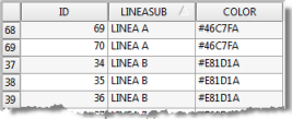
If you are fortunate enough to have this setup and the colors work for you, then you can apply them directly to the color property when you define the layer style. In Leaflet you can use the syntax feature.properties.<PROPERTY> to get the value of any feature attribute:
// Set up styles for subway lines
function subteStyle(feature) {
  return {
    "color": feature.properties.COLOR,
    "weight": 5
  };
}
// Create layer and add it to the map
var subteLayer = L.geoJSON(subteData, {
  style: subteStyle
});
The above code creates a vector layer from the variable subteData which comes from a GeoJSON file. To style the layer, the subteStyle function reads the hex value from the COLOR field and inserts it in the color property of the layer. Notice how the syntax feature.properties.COLOR is utilized to read the color value.
Symbols for unique nominal attributes
Although the above technique is convenient, it's not always practical. What if the colors provided in the file aren't appropriate for your map? Fortunately, in our scenario, you could work around this by providing color values in your JavaScript (i.e., your client-side) code based on the name of the subway line.
Let's look at how you'd apply some style rules on the client side using Leaflet. Examine the following variation on the code we viewed previously. This code produces the exact same map:
// Set up styles for subway lines
function subteStyle(feature) {
  var colorToUse;
  var line = feature.properties.LINEASUB;

  if (line === "LINEA A") colorToUse = "#46C7FA";
  else if (line === "LINEA B") colorToUse = "#E81D1A";
  else if (line === "LINEA C") colorToUse = "#4161BA";
  else if (line === "LINEA D") colorToUse = "#599C65";
  else if (line === "LINEA E") colorToUse = "#65018A";
  else if (line === "LINEA H") colorToUse = "#FAF739";
  else colorToUse = "#000000";

  return {
    "color": colorToUse,
    "weight": 5
  };
}

// Create layer and add it to the map
var subteLayer = L.geoJSON(subteData, {
  style: subteStyle
});
The above example employs a function subteStyle to read the attribute LINEASUB from each feature, thereby figuring out the name of the subway line (LINEA A, LINEA B, etc.). If/then logic is applied to find the appropriate color to use based on the subway line name. Finally, this color is applied to a style returned by the function.
Proportional symbols based on numeric attributes
If you have a field with some numeric attribute, such as the length of a subway line or the number of riders per day, you may want to size the symbols proportionally so that big values are represented with a bigger symbol. Let's consider an example where we have a GeoJSON dataset showing statistics for some of South America's largest metro rail systems. You'll get more familiar with this dataset in the lesson walkthrough, but here's the basic attribute table and map:
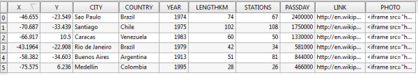
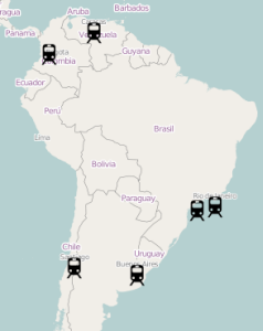
In the above image, the metro systems are all drawn using the same symbol. But let's suppose that you wanted to proportionally size the symbols so that the more stations in a metro system, the larger the map symbol. Notice the STATIONS attribute contains this information. The desired map would look something like the following:
Accomplishing the proportional symbols in Leaflet requires you to define some mathematical function that will size each symbol based on each feature's attribute value for STATIONS. The syntax below is somewhat advanced, but pay attention to the line which reads the value for STATIONS, divides it by 80, and multiplies it by 30 to derive the width and height in pixels for any given metro system symbol. These numbers signify that a metro system with 80 stations will have a symbol 30 pixels wide, a metro system with fewer stations will be less than 30 pixels, and a metro system with more stations will be greater than 30 pixels (the numbers 80 and 30, of course, are entirely arbitrary and could be adjusted to fit your own data):
// function to size each icon proportionally based on number of stations
function iconByStations(feature){
  var calculatedSize = (feature.properties.STATIONS / 80) * 30;

  // create metro icons
  return L.icon({
    iconUrl: 'metro.svg',
    iconSize: [calculatedSize, calculatedSize]
  });
}

// create the GeoJSON layer and call the styling function with each marker
var metroLayer = L.geoJSON(metroData,  {
  pointToLayer: function (feature, latlng) {
    return L.marker(latlng, {icon: iconByStations(feature)});
  }
});
In the above code, iconSize is a two-item JavaScript array containing the width and the height in pixels that should be applied to the icon. Also, notice the use of the pointToLayer property, which is necessary when you want to replace the default Leaflet markers with your own graphics.
Symbols for data classes based on numeric attributes
In some situations, it may be more appropriate to break up your numerical data into various classifications that are symbolized by graduated colors or some similar approach. This is especially true for line and polygon datasets that are sometimes harder to conceptualize using proportional symbols. The boundaries for your classes (in Esri software you may have heard these referred to as "class breaks") could be determined based on equal interval, quantile, natural breaks, or some other arbitrary scheme.
For example, in the image below, metro systems with over 100 stations are symbolized using dark red. Systems with 50 to 100 stations are symbolized with red. Systems with fewer than 50 stations are symbolized with pink:
To symbolize data classes in Leaflet, we'll read one of the feature attributes, then use if/then logic to check it against our class breaks. The code below defines the three classes used in our metro rail example. Each class references a different SVG symbol with its unique hue of red:
// create metro icons
var metroLowIcon = L.icon({
  iconUrl: 'metro_low.svg',
  iconSize: [25,25]
});

var metroMediumIcon = L.icon({
  iconUrl: 'metro_medium.svg',
  iconSize: [25,25]
});

var metroHighIcon = L.icon({
  iconUrl: 'metro_high.svg',
  iconSize: [25,25]
});

// function to use different icons based on number of stations
function iconByStations(feature){
  var icon;
  if (feature.properties.STATIONS >= 100) icon = metroHighIcon;
  else if (feature.properties.STATIONS >= 50) icon = metroMediumIcon;
  else icon = metroLowIcon;

  return icon;
}

// create the GeoJSON layer and call the styling function with each marker
var metroLayer = L.geoJSON(metroData,  {
  pointToLayer: function (feature, latlng) {
    return L.marker(latlng, {icon: iconByStations(feature)});
  }
});
Although the above may look like a lot of code, notice that half of it is just setting up the icons. A function that classified lines or polygons might be much simpler because a single style could be defined with a varying stroke or fill color based on the attribute of interest.
If you intend to use a classification system such as Jenks natural breaks, equal interval, quantile, etc., you must calculate the break values yourself (or find a library [190] that does it) before defining the rules. You can either do this by hand or add more JavaScript code to calculate the values on the fly.
Ways to limit feature visibility based on attributes
In some situations, you may want to display only a subset of the features in a dataset, based on some attribute value or combination of values. (If you're familiar with Esri ArcMap, this is called a "definition query".) Suppose you wanted to show only the metro systems whose COUNTRY attribute was coded as "Brazil":
You can do this directly in the filter property when you create the layer in Leaflet. Here you write a function that evaluates a feature and returns a value of true or false. Leaflet will only draw features for which a value of true is returned:
// create metro icons
var metroIcon = L.icon({
  iconUrl: 'metro.svg',
  iconSize: [25,25]
});


// create the GeoJSON layer and call the styling function with each marker
var metroLayer = L.geoJSON(metroData,  {
  pointToLayer: function (feature, latlng) {
    return L.marker(latlng, {
      icon: metroIcon
    });
  },
  filter: function(feature, layer) {
    if (feature.properties.COUNTRY === "Brazil") return true;
    else return false;
  }
});
The filter function in the above example tests for features where the COUNTRY property equals "Brazil". Note that the above example simply reads an attribute, it does not do a spatial query to find the bounds of Brazil. Your website will run much faster if you can preprocess the data to put a country attribute on each metro system, rather than trying to figure that out on the fly using spatial processing in a web environment.
Now, let's look at a scenario with a numeric attribute. Suppose we wanted to show only the metro systems with over 75 stations:
This could be accomplished with the following filter:
// create metro icons
var metroIcon = L.icon({
  iconUrl: 'metro.svg',
  iconSize: [25,25]
});


// create the GeoJSON layer and call the styling function with each marker
var metroLayer = L.geoJSON(metroData,  {
  pointToLayer: function (feature, latlng) {
    return L.marker(latlng, {
      icon: metroIcon
    });
  },
  filter: function(feature, layer) {
    if (feature.properties.STATIONS > 75) return true;
    else return false;
  }
});
In the code above, note the query for a STATIONS value that is greater than 75.
Conclusion
Leaflet offers a variety of options for symbolizing data on the client side based on attribute values. You should not feel limited to using the default symbology or a single symbol type for the entire layer.
Creating Leaflet styles can require some trial and error, along with some skillful debugging. You'll have more success if you start with a working example and tweak it piece by piece, frequently stopping to test your alterations. This section of the lesson is deliberately code-heavy so that you will have many examples available to get you started.
Spicing up your mapping site with controls
Although Leaflet does not offer a point-and-click interface for building a web application, it does give you a few pre-coded "controls" that you can add to the map with just a few lines of code. These include a scale bar, layer switcher, zoom buttons, and attribution box. OpenLayers offers these same types of controls, plus a few more such as an overview map, geographic coordinates written on the page, and so on.
The example below shows a Leaflet layer switcher control in action. Hovering the mouse over (or tapping) the layer icon in the corner displays a layer list, where you can choose a basemap and toggle the visibility of thematic layers. This image shows the default OpenStreetMap Mapnik basemap selected, with the option to switch to the Stamen Toner basemap. You'll apply this code in your walkthrough later in the lesson. Only one thematic layer is available below, the "Subway lines" layer; however, you could include more layers here simply by adding them to the Leaflet map.
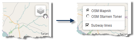
Here's how you would code the layer switcher above. First, set up all the layers and add the ones to the map that you want to have initially visible. Then, call a function that sets up two simple JavaScript objects containing your basemaps and thematic layers. Finally, create the layer switcher (L.control.layers [191]), passing in those two JavaScript objects as parameters.
// create and add osm tile layer
var osm = L.tileLayer('http://{s}.tile.openstreetmap.org/{z}/{x}/{y}.png', {
maxZoom: 19,
attribution: '© <a href="http://www.openstreetmap.org/copyright">OpenStreetMap</a>'
});
osm.addTo(map);
// create stamen osm layer (not adding it to map)
var stamen = L.tileLayer('http://tile.stamen.com/toner/{z}/{x}/{y}.png', {
maxZoom: 19,
attribution: '© <a href="http://www.openstreetmap.org/">OpenStreetMap</a> and contributors, under an <a href="http://www.openstreetmap.org/copyright" title="ODbL">open license</a>. Toner style by <a href="http://stamen.com">Stamen Design</a>'
});
// Set up styles for subway lines
function subteStyle(feature) {
return {
"color": feature.properties.COLOR,
"weight": 5
};
}
// Create layer and add it to the map
var subteLayer = L.geoJSON(subteData, {
style: subteStyle
});
subteLayer.addTo(map);
createLayerSwitcher();
// function to create a layer switcher control
function createLayerSwitcher() {
// define basemap and thematic layers and add layer switcher control
var basemaps = {
"OSM Mapnik": osm,
"OSM Stamen Toner": stamen
};
var overlays = {
"Subway lines": subteLayer
};
L.control.layers(basemaps,overlays).addTo(map);
}
Usually control frameworks are extensible, so you may even decide to pull in controls developed by others or, if you're feeling ambitious, code your own. Although customizing the out-of-the-box Leaflet controls is beyond the scope of this course, you should be aware that controls have a stylesheet you can tweak. Also, controls with images can be customized by substituting your own image. Examining the Leaflet stylesheets and example stylesheets may help you understand which CSS properties to override when applying your customizations.
The Leaflet API reference describes the controls [192] in the namespace L.Control. The best way to learn about controls is to experiment with them yourself and expand your functionality, bit by bit, using existing examples, documentation, and some trial and error. In other web mapping APIs, controls may be called "widgets," "plugins," or other names.
WFS and editing vector data on the web
In Lesson 7, you saw some ways that vector data can be drawn by the web browser or client. The lesson focused on standalone KML and GeoJSON files, yet it is also possible for a web service to send the data to the client on request. The data can be in any format as long as both the server and the client are following the same specification. To standardize the process of sending vector data through web services, the Open Geospatial Consortium (OGC) has produced the Web Feature Service (WFS) specification.
You've already seen a related service, the WMS, in previous lessons. How is WMS different from WFS? WMS involves the server sending a single map image, whereas WFS involves the server sending vector data as text to be drawn by the client. In simple terms, a WMS map is drawn by the server and a WFS map is drawn by the client.
WFS request and response formats
Like a WMS, a WFS supports a set of operations that typically take in parameters directly within the URL. These operations include GetCapabilities, DescribeFeatureType, and GetFeature. The GetFeature operation is the one that actually retrieves features.
Below is an example GetFeatures WFS request for the US state of Colorado (I picked something with a simple geometry). I adapted this from the Boundless WFS tutorial [193], which unfortunately doesn't seem to be available online anymore. Another recommended source for further information on WFS is the OGC e-Learning page [194]. You won't be able to use the link below yourself, but see if you can guess what each parameter signifies, then continue reading about the response:
http://suite.opengeo.org/geoserver/wfs?service=wfs&version=1.1.0&request=GetFeature&typename=usa:states&featureid=states.23
By examining the above URL parameters, you can see that a feature is requested from the WFS using version 1.1.0 of the WFS specification. The service is being hosted on GeoServer in a layer named states in the USA workspace. The feature with index 23 is returned.
A WFS returns data using Geography Markup Language (GML), a specification for expressing GIS data using XML. GML can contain both geometry and attribute information. Because it is based on XML and is designed to be flexible enough to handle many geographic feature types, GML is much more verbose (takes more text) than GeoJSON. Deep down in the GML for Colorado, you can find the geometry:
<gml:posList>37.48468400000007 -109.04348799999995 38.164690000000064 -109.04176199999989 38.27548899999999 -109.06006199999996 41.0006590000001 -109.05007599999999 41.00235900000007 -102.051717 36.993015999999955 -102.04208899999992 36.99908400000004 -109.0452229999999 37.48468400000007 -109.04348799999995</gml:posList>
You can also find attributes like this:
<usa:NAME10>Colorado</usa:NAME10>
The same type of request could be made to one of your own services running on GeoServer. Here's how I made a request for a Philadelphia neighborhood using one of the layers we published earlier in this course:
http://localhost:8080/geoserver/wfs?service=wfs&version=1.1.0&request=GetFeature&typename=geog585:Neighborhoods&featureid=Neighborhoods.12
The response looks like this and contains geometry and attributes for the Olney neighborhood:
<wfs:FeatureCollection numberOfFeatures="1" timeStamp="2014-03-03T15:07:31.822Z" xsi:schemaLocation="http://localhost:8080/geoserver/geog585 http://localhost:8080/geoserver/wfs?service=WFS&version=1.1.0&request=DescribeFeatureType&typeName=geog585%3ANeighborhoods http://www.opengis.net/wfs http://localhost:8080/geoserver/schemas/wfs/1.1.0/wfs.xsd"><gml:featureMembers><geog585:Neighborhoods gml:id="Neighborhoods.12"><geog585:the_geom><gml:MultiSurface srsDimension="2" srsName="urn:x-ogc:def:crs:EPSG:3857"><gml:surfaceMember><gml:Polygon srsDimension="2"><gml:exterior><gml:LinearRing srsDimension="2"><gml:posList>-8363968.786751106 4869301.13520122 -8363706.077778376 4871057.31164155 -8363880.846283749 4871132.918517317 -8363697.377540309 4872031.511981935 -8363780.660729433 4872179.806916264 -8363847.448310932 4872208.890548547 -8363802.926044645 4872557.878939522 -8363802.44449278 4872626.491915396 -8363025.915000884 4872530.247301338 -8361543.138729884 4872310.6731403675 -8361453.88028348 4872223.294811407 -8361493.045963939 4872015.489274301 -8361627.94355705 4871826.7318475135 -8361690.687270048 4871673.398417745 -8361627.94355705 4871403.748827802 -8361286.901117077 4870791.777211798 -8361326.368936536 4870458.7113405885 -8361498.408149585 4869986.8871721085 -8361555.111808623 4869831.380121785 -8362695.297708079 4869623.850560427 -8363168.406381819 4869548.2551895585 -8363968.786751106 4869301.13520122</gml:posList></gml:LinearRing></gml:exterior></gml:Polygon></gml:surfaceMember></gml:MultiSurface></geog585:the_geom><geog585:STATE>PA</geog585:STATE><geog585:COUNTY>Philadelphia</geog585:COUNTY><geog585:CITY>Philadelphia</geog585:CITY><geog585:NAME>Olney</geog585:NAME><geog585:REGIONID>214146.0</geog585:REGIONID></geog585:Neighborhoods></gml:featureMembers></wfs:FeatureCollection>
WFS servers and clients
Although the syntax for WFS requests and responses may look intimidating, you will rarely have to worry about composing this yourself. Various FOSS and proprietary software packages include support for viewing and serving WFS.
WFS servers
As shown in the above examples, GeoServer can expose your layers through WFS. This is enabled by default and requires no configuration on your part. Other FOSS GIS servers such as Map Server and Deegree support the creation of WFS web services.
In the proprietary realm, Esri ArcGIS Server gives users the option to expose their web services through WFS; however, Esri has developed its own "feature service" that works through REST and accomplishes many of the same things as a WFS. Be aware that the Esri web mapping APIs and editing widgets are designed to work with the feature service rather than WFS. The communication patterns of the feature service are openly documented in the GeoServices REST Specification.
WFS clients
Support for WFS varies across web mapping APIs. WFS can be viewed "out of the box" as a vector layer in OpenLayers, but not within Leaflet. As mentioned above, Esri web mapping APIs are designed to work with the REST feature service rather than WFS.
Although Leaflet won't draw the GML responses sent by a WFS, it will draw GeoJSON; therefore, one pattern of working with WFS via Leaflet is to configure the server to send back GeoJSON instead of GML. You can then send WFS requests to the server via AJAX (asynchronous web requests) and use Leaflet classes to draw the geoJSON coming back. Such patterns are exposed through numerous forum posts [195], as well as third-party plugins.
On the desktop side, QGIS supports viewing and editing WFS. (Note: I got errors when trying to edit a WFS in QGIS, but I did not have a database or proxy host behind the layer.) Other FOSS clients such as uDig also recognize the WFS format. In Esri ArcMap, you use the Data Interoperability Extension to add WFS layers to the map (see "Connecting to a WFS Service [196]"). ArcGIS Pro allows users to add WFS, and the extension does not appear to be required (documentation here [197]).
Transactional WFS (WFS-T) and web-based editing
The WFS specification also defines rules for feature editing, opening the door to building clients that can edit geographic data over the web. A WFS enabled for editing is known as a transactional WFS, or WFS-T. Beyond the standard WFS operations such as GetFeature, WFS-T supports an additional operation called Transaction, and may also support operations for locking features to prevent concurrent edits.
Creating web editing applications requires both a server that can handle the incoming transactions and a client that provides visual support for the edit sketching, vertex manipulation, attribute entrance into text boxes, and so forth. The client sketching operations must be wired up to the WFS-T requests. Unless you're ready to write a lot of JavaScript, it's best to start with existing samples, widgets, or web controls. Leaflet offers a Draw control [198] that can take care of the sketching part. See an example of what "Draw" [199] can do. The respec/leaflet.wfs-t [200] is an example of a plugin designed to wire up the Draw control to WFS-T requests. (Full disclosure: I have not tested this particular plugin, but there are other plugins based on the same concept).
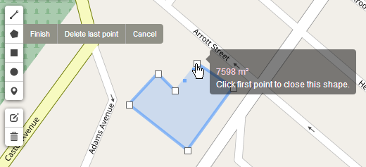
OpenLayers also offers some basic buttons for sketching, modifying, deleting, and saving features. You can see them in action in this developer example [201].
Before you expose any dataset for editing over the web, you should carefully think through your quality control and data storage architectures. For example, perhaps you want to expose a copy of your database for web editing, then have an analyst review any changes before they are pushed to your master GIS database. If in-house editors are making changes to the master database, you'll also need a way to periodically push those to your web copy. In other cases, you may check incoming edits with a script to make sure they comply with certain topology rules or attribute schema requirements.
WPS, Turf.js, and spatial data processing on the web
Both FOSS and proprietary GIS software offer spatial data processing functions such as buffer, union, contour, interpolate, and so on. You invoked some of these using QGIS and GDAL in earlier lessons. But what if you wanted to allow people to run these functions from a web browser? For example, suppose you wanted to allow users of your web map to draw a polygon and then see a calculation of the total population and number of health clinics within that polygon. You'd be able to expose the GIS to many people without them needing to install any GIS software.
OGC has released a specification for invoking spatial data processing through web services. It's called the Web Processing Service (WPS) specification. Like the other OGC services you've learned about, it offers a set list of operations you can call. These are: GetCapabilities, DescribeProcess, and Execute. Of course, the Execute operation is the one that launches the request to actually perform the processing. The server does the work to process the data and send back the result as a response. GML may be used to transfer information about vector features in either the request or the response.
As you are probably aware from running GDAL and ArcToolbox tools, spatial data processing functions can sometimes require many input parameters. For example, a buffer process might require you to specify the width of the buffer, whether it will be applied to both sides of the feature, whether the ends should be capped or rounded, etc. Each tool has its own set of parameters and syntax for describing them. Because the inputs can be so long and complex (especially if geometry is included), sometimes you can put the inputs in their own XML file and POST them to the server, rather than putting all the parameters into the URL as a GET request like you have seen with WMS and WFS in previous lessons. Some servers and browsers impost limits on the length of an HTTP GET request, whereas HTTP POST requests can typically be much longer.
The WPS spec itself doesn't say which types of spatial data processing operations a WPS must support; that's up to whoever builds and administers the service. There are hundreds of potential operations that can be included. When you first use a WPS, you can invoke the GetCapabilities operation to find out which processes are available.
WPS servers
GeoServer offers a WPS extension [202] that exposes a set of spatial processes from the FOSS JTS Topology Suite [203], as well as some other processes developed specifically by GeoServer. We will not install this extension in this course, but I encourage you to browse through the documentation if you think that you may use it in your workplace or other academic work.
The Zoo Open WPS Platform [204] and PyWPS [205] are other examples of FOSS WPS implementations. In the proprietary realm, Esri ArcGIS Server can serve a WPS from a ModelBuilder model that you create from ArcToolbox tools or scripts.
WPS clients
A few GUI-based WPS clients are available that allow you to select tools and supply their parameters in text boxes or dropdown lists. QGIS has a WPS plugin [206] that works this way, allowing you to call a WPS from the desktop.
When it comes to invoking a WPS directly from a web application, some web map APIs offer helper classes or libraries that can help you. Leaflet is not one of these (I will get to that in a minute). OpenLayers 2 supports WPS through the use of OpenLayers.WPSClient. When you instantiate this object, you supply the URL of the WPS server. You then set up JavaScript objects containing all the parameters of the process you want to invoke. Finally, you execute the process and specify what should be done with the results. See this OpenLayers developer example [207]available online.
Even when you use a WPS client plugin, library, or object, you still need to be familiar with the process and its documentation, so that you can supply the correct syntax for the parameters. One mistake in syntax can derail the entire processing operation. Furthermore, WPS servers and clients are often either in the early stages of maturity or are designed for power users who are comfortable with a lack of a GUI and extensive documentation.
Turf.js as a WPS alternative
Many spatial processing operations are rather common, and there is a great desire from GIS web developers to invoke these without the overhead of a WPS. The Turf.js [208] library has gained popularity for allowing geoprocessing directly on GeoJSON vectors in a JavaScript environment. In other words, Turf differs from WPS because the client machine runs the processing code, not the server. Turf was developed at Mapbox, but is free to use and modify under the open MIT license [209]. Operations available through Turf.js include dissolving, unioning, intersecting, buffering, aggregating, calculating centroids, and so forth.
You can download Turf.js to your own machine or access it online via a CDN [210]. Because Turf.js works on GeoJSON, it fits very nicely with Leaflet. Most of the abundant Turf.js developer examples are shown using Mapbox's API (for obvious reasons), but the way you would invoke them from Leaflet is essentially the same. For example, the following snippet is from the Turf.js analysis walkthrough [211]:
  // Using Turf, find the nearest hospital to library clicked
  var nearestHospital = turf.nearest(e.layer.feature, hospitalFeatures);
In this situation, both parameters of the turf.nearest() function are GeoJSON objects: one representing a library building, and another one representing a set of hospital buildings. The function finds the hospital nearest the clicked library and returns it as GeoJSON. Fundamentally, it doesn't matter which API you use to display the output GeoJSON.
Performance considerations
Before implementing any kind of spatial data processing on the web, consider ways that you might preprocess the data in order to eliminate the need for on-the-fly calculations. When you invoke spatial processing on the web, it makes your server busy and increases end-user wait times. In the above example, perhaps the nearest hospital to each library could be precalculated in a desktop GIS environment and stored in the library attribute table. Then your code would just need to read the attribute, rather than performing processing.
There will be some situations where precalculation doesn't make sense due to the wide range of analysis parameters and possibilities you want to expose. For example, if there were 20 different kinds of features that you wanted to allow people to find near a library, or if a person could type in the address of some library not in the original dataset. Therefore, the decision about whether to allow real-time spatial processing should be made on a case-by-case basis.
Implementing spatial data processing in the term project
Unless you already have some previous exposure to WPS, I do not recommend integrating it into your term project given the short amount of time that remains in the course. A Turf.js implementation would be a better fit for the scope of the term project, since it can be implemented fairly quickly with less code.
Neither of these technologies is a requirement for the project, although they may provide useful functionality in many scenarios.
JavaScript libraries and web presentation frameworks
Working with web pages is not always easy, especially when it's not your main area of expertise. Code for laying out the page, iterating through elements, toggling classes, etc., can get clunky and bloated in a hurry. Browsers can interpret the same pieces of HTML and JavaScript differently, and debugging the pages can be a mysterious process involving multiple code files and complex hierarchies of stylesheets and overrides.
There is no magic solution for these challenges; however, there are some JavaScript helper libraries that can simplify your life and your code if you make the effort to learn them. Your pages will probably also become more functional and attractive. Some of these libraries offer mainly back-end functions, others specialize in front-end elements, and others offer both.
JavaScript libraries
Many web developers like to use special JavaScript libraries that have been developed to simplify common functions and abstract away some of the idiosyncrasies between web browsers.
For example, if you select a few web pages at random and look at the source code, chances are pretty good that you'll see someone using the jQuery library. jQuery [212] provides functions to simplify navigating and manipulating the DOM elements on your page. For example, using jQuery you can populate a dropdown list or change the CSS class of an HTML element on the fly without writing a bunch of HTML markups.
Similar alternatives to jQuery are Prototype [213] and the Dojo toolkit [214], although the latter also offers some UI elements such as menus, buttons, and charts. All these libraries are build with the goal of simplifying JavaScript coding and reducing the work for you to handle differences between browsers.
Web presentation frameworks
In the previous lesson examples, you've learned how to embed your map in a web page. In the Lesson 7 walkthrough, you also briefly saw how to use the innerHtml property to manipulate a DOM element and thereby change a label on a page. But how do you craft a nice looking page around your map without devoting hundreds of hours to web design study? This is where a web presentation framework can come in handy.
Web presentation frameworks consist of JavaScript libraries, stylesheets, and "widgets" that work together to give you some convenient building blocks for nice looking pages. Some of these goodies include headers, buttons, calendar date pickers, menus, etc.
Web development frameworks are typically engineered so that your page works in a similar manner across browsers. They may also give you a head start with making your page easily localizable (i.e., flexible enough to be offered in various languages such as Spanish, Arabic, Chinese, etc.).
Examples
An example of a popular web presentation framework is Bootstrap [215], distributed by the Twitter development team under an open source license. In the Lesson 8 walkthrough, you'll use Bootstrap to put a nice header on your application and divide your page into sections. You'll also get the benefit of the Bootstrap stylesheets.
Similar frameworks to Bootstrap include Groundwork [216], Zurb's Foundation [217], and Yahoo's Pure [218]. The latter used to be called YUI (yoo'-ee) and this name is still often seen in the web world. Take a few minutes and follow some of the above links to see the different styles offered by these frameworks.
Some JavaScript libraries such as the Dojo toolkit and Sencha Ext JS [219] also offer layout elements that serve a web design function. The project jQuery UI [220] offers a helpful set of user interface elements such as buttons, menus, date pickers, etc.
Even more powerful, we have web application frameworks for supporting the design and implementation of complex web applications and services, like the popular Python-based Django [221] and JavaScript-based React [222], which also contain web presentation components.
You should be aware that web presentation frameworks sometimes require and use jQuery or other libraries to accomplish their functions.
Choosing a framework
When evaluating a web presentation framework for your project, you might consider:
- How easy is it to get started with the framework?
- How many online examples are available on the framework and is there an active community posting to forums, etc.?
- How easy is it to customize the framework if I don't like the default choices or examples?
- Is the framework hosted on a CDN or do I have to host it myself? Hosting yourself is often required anyway if you want to customize or slim down any portion of the framework, but it does take more work.
- What are the terms of use for this framework, including attribution and licensing requirements? Just like other kinds of software, there are FOSS frameworks and proprietary ones.
A web presentation framework can help produce a nicer end product than you might be able to concoct on your own; however, a framework also introduces another level of complexity. You may have to override some of the framework's stylesheets in order to get other libraries (like Leaflet or OpenLayers) to behave in the expected way. Debugging such issues often involves multiple levels of stylesheets and a lot of time in the weeds. If you just need a very simple app, you might leave the framework aside and create your own stylesheet, or at least try to select the most simple framework available for the functionality you need.
Walkthrough: Thematic map with Leaflet controls and Bootstrap framework
In this walkthrough, you'll put together some of the things you've learned in this lesson to make a well-rounded informational map containing thematic styling and Leaflet controls. The map will use the Bootstrap web presentation framework so that it can be extended with supplementary content in an aesthetically pleasing way. You will construct some of this content on the fly by reading the attributes of selected map features.
For this exercise, we'll stick with the metro data from South America. The final application will allow users to click any metro and see some informational text and an image from Flickr. A static legend image is also brought into the layout.
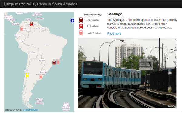
Although this lesson is called "Going beyond 'dots on a map," I have deliberately chosen point data for this walkthrough so that you can appreciate the possibilities offered through Leaflet, especially when tied together with other frameworks. Although you may not feel like a JavaScript guru at this point, you should at least know that you don't have to settle for the 'red teardrop and popup' mashups that you see all over the Internet.
Downloading the data and examining the layout
- Download the Lesson 8 walkthrough data [223] and unzip it anywhere. If you like, you could place the files in your Jetty home folder, but the walkthrough does not use GeoServer and this is not required. The files include a legend image, the metro SVG images, and a GeoJSON file of metro locations and attributes. Notice that in a departure from previous walkthroughs, I've already supplied an HTML file containing the basic layout markup. We will examine some of the key pieces of the markup in the steps below. You'll also add some JavaScript to give this app some life. Also, please note that the files include a style.css file like we used in the previous lessons, but with one important change: The width attribute of the map has been changed from a fixed absolute number of pixels to a relative value (90%) to make sure that the div section for the map will work together with the Bootstrap layout template we will use in this walkthrough.
- Open lesson8_walkthrough.html in a web browser and take a look. You should see the empty shell of the app with no map yet.
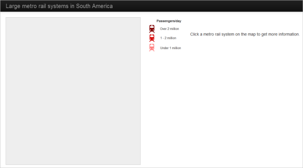 Figure 8.13.
 - Open lesson8_walkthrough.html in your favorite text editor and look over the HTML markup. The layout is based on an old OpenLayers and Bootstrap example that doesn't seem to be available online anymore.
Before you add JavaScript, I will just point out a few things that are important in the layout. First, notice how Bootstrap is brought into the application through a reference to a JavaScript file (.js) and a CSS file (.css) in the bolded lines below. We are referencing the files from a CDN, but you could alternatively download and host (and tweak) them yourself.
<script src="http://code.jquery.com/jquery-latest.js"></script>
. . .
<script src="https://maxcdn.bootstrapcdn.com/bootstrap/2.2.1/js/bootstrap.min.js"></script>
<link rel="stylesheet" href="https://maxcdn.bootstrapcdn.com/bootstrap/2.2.1/css/bootstrap.min.css">
Also take note of the stylesheet override in the <style> tag. This will prevent our page content from crashing into the top banner.
<style>
  body {
    padding-top: 60px;
    padding-bottom: 40px;
  }
</style>
If you don't like something about the Bootstrap (or Leaflet) default styles, the stylesheet overrides are where you can apply a change.
In the page body, observe how classes are used to organize the page into navigation bars (navbar-*), containers (container-fluid), and spans. The span5 and span7 classes divide the page vertically so that consistent proportions of the page area are devoted to the map (on the left) and the supplementary material (on the right). Don't worry about understanding all these classes at this point. Just be aware that web development frameworks like Bootstrap, Dojo, etc., may give you CSS classes for organizing page elements in a way that should behave consistently across browsers.
Finally, note that the legend image and the "Click a metro..." text are organized into an HTML table to keep them flush. The table borders are invisible by design.
<table>
  <tr>
    <td><img src="metro_legend.png"/></td>
    <td id = 'summaryLabel'><p>Click a metro rail system on the map to get more information.</p></td>
  </tr>
</table>
A div awaits for a Flickr image, but this won't appear until someone clicks a metro symbol on the map.
<div id="metroImage"></div>
Now let's breathe some life into this app by adding some JavaScript code.
Adding the JavaScript logic
You'll use JavaScript to do three main things in this application: add the map, define the symbols, and handle the click events. Let's address these in order.
-
In your lesson8_walkthrough.html, find the script tags. You'll put all your code immediately after: <script type="text/javascript">.
-
Add the following lines of code to create the map and an initialization function. This function contains some variables that we'll use to handle selections throughout, similar to what you saw in Lesson 7:
var map; var metroLayer; function init() { // create map and set center and zoom level map = new L.map('mapid'); map.setView([-28,-62],3); var selection; var selectedLayer; var selectedFeature; . . . } - Now let's create some layers and put them on the map. The code below creates two tiled basemap layers and the metro layer. It only adds one basemap layer to the map; the other one will eventually be an option in the layer switcher.
One more note regarding the two basemap layers: Until recently, we used the standard OSM basemap as the first basemap option and the dark-themed Stamen Toner basemap as the second option in this walkthrough. However, since November 2023 the Stamen basemap tiles are not hosted by Stamen anymore but instead are provided by a company called Stadia as part of one of the plans they are offering to their customers, including a free plan for up to 200,000 requests (see this page for details: https://docs.stadiamaps.com/guides/migrating-from-stamen-map-tiles/ [224]). We therefore changed this walkthrough to use a second OSM basemap called OSM Humanitarian as the second option. If you instead would like to use the original Stamen Toner basemap, what you can do is follow the steps described on the migration page linked above: (1) create a Stadia account and pick the free plan, (2) pick the option to use an API key to access their tiles, and (3) use the following URL for the second basemap option in the code below replacing xyz with your API key:'https://tiles.stadiamaps.com/tiles/stamen_toner/{z}/{x}/{y}.png?api_key=xyz'Now replace the . . . in the code above with the following. Although it's a lot, all of this should look pretty familiar if you paid attention to the code snippets earlier in the lesson:// create and add osm tile layer var osm = L.tileLayer('https://{s}.tile.openstreetmap.org/{z}/{x}/{y}.png', { maxZoom: 19, attribution: '© <a href="http://www.openstreetmap.org/copyright">OpenStreetMap</a>' }); osm.addTo(map); // create osm humanitarian layer (not adding it to map) var osmHumanitarian = L.tileLayer('https://{s}.tile.openstreetmap.fr/hot/{z}/{x}/{y}.png', { maxZoom: 19, attribution: '© <a href="http://www.openstreetmap.org/copyright">OpenStreetMap</a>' }); // create metro icons var metroLowIcon = L.icon({ iconUrl: 'metro_low.svg', iconSize: [25,25] }); var metroMediumIcon = L.icon({ iconUrl: 'metro_medium.svg', iconSize: [25,25] }); var metroHighIcon = L.icon({ iconUrl: 'metro_high.svg', iconSize: [25,25] }); var metroSelected = L.icon({ iconUrl: 'metro_selected.svg', iconSize: [25,25] }); // add the metro GeoJSON layer var metroLayer = L.geoJson(metroData,{ pointToLayer: function (feature, latlng) { return L.marker(latlng, {icon: iconByPassday(feature)}); }, onEachFeature: metrosOnEachFeature }); metroLayer.addTo(map); . . .You may have noticed that the metroLayer relies on two functions: iconByPassday and metrosOnEachFeature. We'll tackle those in a few minutes. But first, the layer switcher...
-
Replace the . . . in the code above to add a layer switcher control to the map:
// define basemap and thematic layers and add layer switcher control
var basemaps = {
  "OSM": osm,
  "OSM Humanitarian": osmHumanitarian
};

var overlays = {
  "Metro stations": metroLayer
 };

L.control.layers(basemaps,overlays).addTo(map);

. . .
Again, the pattern here is to create a JavaScript object for the basemaps and one for the thematic layers, and then pass those two objects in as parameters when you create the control. -
Now for those functions I mentioned. The first one, iconByPassday, looks at the number of passengers per day that travel through each metro system, then decides which icon to use. It's the key to classifying the layer and symbolizing it with the different colors. Replace the . . . in the code above with the following:
// define functions that right icon for a given feature function iconByPassday(feature) { var icon; if (feature.properties.PASSDAY >= 2000000) icon = metroHighIcon; else if (feature.properties.PASSDAY >= 1000000) icon = metroMediumIcon; else icon = metroLowIcon; return icon; } . . . -
Now for that metrosOnEachFeature function. This one is a little more lengthy. It adds a click event listener to the metros layer and then defines a function to handle that event. Replace the . . . in the code above with the following:
// define function to handle click events on metro features
function metrosOnEachFeature(feature, layer){
  layer.on({
    click: function(e) {
      // reset symbol of old selection
      if (selection) {
        if (selectedLayer === metroLayer) selection.setIcon(iconByPassday(selectedFeature));
      }

      // apply yellow icon to newly selected metro and update selection variables
      e.target.setIcon(metroSelected);
      selection = e.target;
      selectedLayer = metroLayer;
      selectedFeature = feature;

      // using attributes, construct some HTML to write into the page
      var featureName = feature.properties.CITY || 'Unnamed feature';
      var country = feature.properties.COUNTRY || '(Unknown)';
      var year = feature.properties.YEAR || '(Unknown)';
      var passengers = feature.properties.PASSDAY || '(Unknown)';
      var stations = feature.properties.STATIONS || '(Unknown)';
      var length = feature.properties.LENGTHKM || '(Unknown)';
      var link = feature.properties.LINK || 'http://www.wikipedia.org';
      var photoHtml = feature.properties.PHOTO || '<P>Photo not available</P>';
      var titleHtml = '<p style="font-size:18px"><b>' + featureName + '</b></p>';
      var descripHtml = '<p>The ' + featureName + ', ' + country + ' metro opened in ' + year + ' and currently serves ' + passengers + ' passengers a day. The network consists of ' + stations + ' stations spread over ' + length + ' kilometers.</p>';
      var readmoreHtml = '<p><a href="' + link + '">Read more</a></p>';
      document.getElementById('summaryLabel').innerHTML = titleHtml + descripHtml + readmoreHtml;
      document.getElementById('metroImage').innerHTML = photoHtml;

      L.DomEvent.stopPropagation(e); // stop click event from being propagated further
    }
  });
}

. . .
Examine the code comments above to understand what each section is doing. There's a lot of code, but most of it is constructing the informational HTML describing the metro system. Recall that the attribute table looks like this:
Figure 8.15.You should notice many of these attribute field names referenced in the code above. The field value is retrieved, using some special syntax || (logical OR operator that in JavaScript returns the first operand that is TRUE) to set a fallback value in case no attribute comes back. The rest of the function constructs some HTML strings, inserting the attributes where appropriate. After the HTML strings are constructed, the innerHTML is updated for the elements "summaryLabel" and "metroImage." This causes the new text and the photo to appear on the right side of the page.
The PHOTO field deserves some additional discussion here. Anticipating that this field would be used to embed a photo in an app, the entire iframe HTML code is placed in this field as a long string. Where do you get this code if you want to make a dataset like this? Right from the Flickr embed functionality: Figure 8.16.
 -
Finally, add a click event handler to the map that will reset the selection. This is necessary if someone clicks the map, but not a metro icon. Replace the . . . in the code above with the following:
// define and register event handler for click events to unselect features when clicked anywhere else on the map
map.addEventListener('click', function(e) {
  if (selection) {
    if (selectedLayer === metroLayer) selection.setIcon(iconByPassday(selectedFeature));

    selection = null;

    document.getElementById('summaryLabel').innerHTML = '<p>Click a metro rail system on the map to get more information.</p>';
    document.getElementById('metroImage').innerHTML = ''
  }
});
Notice that some code was added here to also clear out the informational HTML and the photo. -
Test the application by opening lesson8_walkthrough.html in a web browser. (If you're just opening the HTML file directly from the file system, I recommend using Firefox to test. This is because the cross-origin request security implementations in Chrome and Internet Explorer only allow the GeoJSON to load if you're hosting both the HTML and GeoJSON files on a web server.)
You should be able to switch between different base layers (note that the Map Quest open layer shown below is no longer available). Click a metro icon to see the highlighted symbol, the Flickr image, and the descriptive text.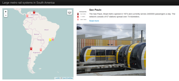 Figure 8.17.
Final code for the walkthrough
If the walkthrough does not function, check to ensure you are connected to the Internet and that your code matches the code below:
<!DOCTYPE html>
<html>
<head>
<meta http-equiv="Content-Type" content="text/html; charset=utf-8">
<title>Lage metro rail systems in South America</title>
<link rel="stylesheet" href="https://cdnjs.cloudflare.com/ajax/libs/leaflet/1.2.0/leaflet.css" type="text/css" crossorigin="">
<script src="https://cdnjs.cloudflare.com/ajax/libs/leaflet/1.2.0/leaflet.js" crossorigin=""></script>
<script src="http://ajax.googleapis.com/ajax/libs/jquery/1.9.1/jquery.min.js"></script>
<script src="metro.js"></script>
<link rel="stylesheet" href="style.css" type="text/css">
<script src="https://maxcdn.bootstrapcdn.com/bootstrap/2.2.1/js/bootstrap.min.js"></script>
<link rel="stylesheet" href="https://maxcdn.bootstrapcdn.com/bootstrap/2.2.1/css/bootstrap.min.css">
<style>
body {
padding-top: 60px;
padding-bottom: 40px;
}
</style>
<script type="text/javascript">
var map;
var metroLayer;
function init() {
// create map and set center and zoom level
map = new L.map('mapid');
map.setView([-28,-62],3);
var selection;
var selectedLayer;
var selectedFeature;
// create and add osm tile layer
var osm = L.tileLayer('https://{s}.tile.openstreetmap.org/{z}/{x}/{y}.png', {
maxZoom: 19,
attribution: '© <a href="http://www.openstreetmap.org/copyright">OpenStreetMap</a>'
});
osm.addTo(map);
// create osm humanitarian layer (not adding it to map)
var osmHumanitarian = L.tileLayer('https://{s}.tile.openstreetmap.fr/hot/{z}/{x}/{y}.png', {
maxZoom: 19,
attribution: '© <a href="http://www.openstreetmap.org/copyright">OpenStreetMap</a>'
});
// create metro icons
var metroLowIcon = L.icon({
iconUrl: 'metro_low.svg',
iconSize: [25,25]
});
var metroMediumIcon = L.icon({
iconUrl: 'metro_medium.svg',
iconSize: [25,25]
});
var metroHighIcon = L.icon({
iconUrl: 'metro_high.svg',
iconSize: [25,25]
});
var metroSelected = L.icon({
iconUrl: 'metro_selected.svg',
iconSize: [25,25]
});
// add the metro GeoJSON layer
var metroLayer = L.geoJson(metroData,{
pointToLayer: function (feature, latlng) {
return L.marker(latlng, {icon: iconByPassday(feature)});
},
onEachFeature: metrosOnEachFeature
});
metroLayer.addTo(map);
// define basemap and thematic layers and add layer switcher control
var basemaps = {
"OSM": osm,
"OSM Humanitarian": osmHumanitarian
};
var overlays = {
"Metro stations": metroLayer
};
L.control.layers(basemaps,overlays).addTo(map);
// define functions that right icon for a given feature
function iconByPassday(feature) {
var icon;
if (feature.properties.PASSDAY >= 2000000) icon = metroHighIcon;
else if (feature.properties.PASSDAY >= 1000000) icon = metroMediumIcon;
else icon = metroLowIcon;
return icon;
}
// define function to handle click events on metro features
function metrosOnEachFeature(feature, layer){
layer.on({
click: function(e) {
// reset symbol of old selection
if (selection) {
if (selectedLayer === metroLayer) selection.setIcon(iconByPassday(selectedFeature));
}
// apply yellow icon to newly selected metro and update selection variables
e.target.setIcon(metroSelected);
selection = e.target;
selectedLayer = metroLayer;
selectedFeature = feature;
// using attributes, construct some HTML to write into the page
var featureName = feature.properties.CITY || 'Unnamed feature';
var country = feature.properties.COUNTRY || '(Unknown)';
var year = feature.properties.YEAR || '(Unknown)';
var passengers = feature.properties.PASSDAY || '(Unknown)';
var stations = feature.properties.STATIONS || '(Unknown)';
var length = feature.properties.LENGTHKM || '(Unknown)';
var link = feature.properties.LINK || 'http://www.wikipedia.org';
var photoHtml = feature.properties.PHOTO || '<P>Photo not available</P>';
var titleHtml = '<p style="font-size:18px"><b>' + featureName + '</b></p>';
var descripHtml = '<p>The ' + featureName + ', ' + country + ' metro opened in ' + year + ' and currently serves ' + passengers + ' passengers a day. The network consists of ' + stations + ' stations spread over ' + length + ' kilometers.</p>';
var readmoreHtml = '<p><a href="' + link + '">Read more</a></p>';
document.getElementById('summaryLabel').innerHTML = titleHtml + descripHtml + readmoreHtml;
document.getElementById('metroImage').innerHTML = photoHtml;
L.DomEvent.stopPropagation(e); // stop click event from being propagated further
}
});
}
// define and register event handler for click events to unselect features when clicked anywhere else on the map
map.addEventListener('click', function(e) {
if (selection) {
if (selectedLayer === metroLayer) selection.setIcon(iconByPassday(selectedFeature));
selection = null;
document.getElementById('summaryLabel').innerHTML = '<p>Click a metro rail system on the map to get more information.</p>';
document.getElementById('metroImage').innerHTML = ''
}
});
}
</script>
</head>
<body onload="init()">
<div class="navbar navbar-inverse navbar-fixed-top">
<div class="navbar-inner">
<div class="container-fluid">
<a class="brand" href="/">Large metro rail systems in South America</a>
</div>
</div>
</div>
<div class="container-fluid">
<div class="row-fluid">
<div class="span5">
<div id="mapid">
</div>
</div>
<div class="span7">
<div>
<table>
<tr>
<td><img src="metro_legend.png"/></td>
<td id = 'summaryLabel'><p>Click a metro rail system on the map to get more information.</p></td>
</tr>
</table>
<div id="metroImage"></div>
</div>
</div>
</div>
</div>
</body>
</html>
Lesson 8 assignment: Independent exploration of FOSS
If the amount of JavaScript in the walkthrough was intimidating, don't worry. You don't have to write that kind of code in the lesson assignment, although I hope some of it comes in handy in your term project.
For this week's assignment, we're going to do something a bit different. You will identify and report on some GIS FOSS that interests you. Your typical encounter with FOSS in the "real world" will be open-ended, with little direction other than what you can find online. Therefore, this assignment is designed to give you an experience of independent exploration.
Reading
First, read this article to get an idea of the many different FOSS products used with GIS, some of which we have not covered in this course. I have placed this article in the Lesson 8 module in Canvas:
- Steiniger, S., & Hunter, A. J. (2013). The 2012 free and open source GIS software map–A guide to facilitate research, development, and adoption. Computers, Environment and Urban Systems, 39, 136-150.
With its many acronyms, this article approaches alphabet soup at times. But I think you are far enough along in this course that you will recognize some of them and have enough frame of reference to process the ones you don't know. Obviously, this article is several years old, but will help get you up to date on the major players in FOSS GIS. I am not aware of a more recent article as thorough as this.
Experimentation
Identify a FOSS solution for GIS that we have not covered in this course, download it (if applicable), and briefly experiment with it. Then use the software to accomplish something useful.
In fulfilling this requirement, keep in mind the following:
- This should ideally be some software that will be helpful in your term project, although this is not required.
- APIs, such as OpenLayers and D3, are okay for this requirement.
- If you select a cloud-based service, be sure that it contains some open source element.
Use the Steiniger and Hunter article, as well as the Ramsey video from Lesson 1, if you need ideas about what to review.
Deliverable
Write a report of around 1000 words describing the following:
- What software you chose, who makes it, and why.
- How it relates to web mapping.
- What useful function you accomplished with it. Provide screenshots.
- What documentation you found and used in accomplishing the above things. Provide links. Please also comment on its quality.
- How this software could possibly complement or extend the projects you have completed in this course.
If you reviewed a cloud based service or a FOSS product created by a for-profit entity, please delineate which elements of the software are FOSS and which are not. Also describe how the FOSS portion fits into the business model of the provider.
Remember that free software and APIs are not always open source. The software you review for this assignment must have some portion where the source code is openly shared and can be reused or modified.
You should submit your report into the Lesson 8 assignment drop box on Canvas.
Lesson 9: Exploring open data, VGI, and crowdsourcing
The links below provide an outline of the material for this lesson. Be sure to carefully read through the entire lesson before returning to Canvas to submit your assignments.
Note: You can print the entire lesson by clicking on the "Print" link above.
Overview
A GIS or web map is only as useful as the data you put into it. Just as the GIS landscape offers proprietary software and open software, you will see sources of proprietary data and open data. This lesson explores the different meanings of "open data" and provides an introduction to OpenStreetMap, a growing repository of open data that is useful in a variety of projects.
Objectives
- Define “open data” and describe some of the differences in use conditions among open data options.
- Recognize the benefits and weaknesses of OpenStreetMap and its process of crowdsourcing.
- Describe options for retrieving data from OpenStreetMap.
- Edit OpenStreetMap according to community-defined tagging standards, and describe what you learned about open data sources from this experience.
Checklist
- Read the Lesson 9 materials on this page.
- Complete the walkthrough.
- Complete the Lesson 9 assignment.
- Complete the "third quiz" on Canvas. This covers material from Lessons 7 - 9.
Ways of opening data
Lately, it seems that "open data" is everywhere. Reaching buzzword status, this term is often seen in tandem with phrases such as "open government," "crowdsourcing," "government transparency," and "free and open source software." But what makes data "open"? Just as you learned in Lesson 1, that different organizations, even proprietary software companies, employ the term "open source" to their advantage. There are various nuances to the term "open data" that you should consider whenever you hear someone touting this phrase.
Consider the following means of data access and how they might be placed on a continuum of more or less "open":
- The data is not available in any format for the public to view or download (the baseline case of "closed" data).
- The data is distributed in static format only, such as a paper map or PDF.
- The data can be viewed by anyone through a web map, but not downloaded.
- The data can be accessed by anyone through a web service and displayed in a GIS or web map, but the full dataset cannot be downloaded.
- The data can be downloaded in proprietary data formats at no cost.
- The data can be downloaded in open formats at no cost.
Consider how these levels of data access play into the following scenarios:
- A person exposing a dataset claims that "the data is open because I let you see the data;" however, the data itself may not be available for download due to licensing, security, technical, or human resources restrictions.
- An "open data portal" might expose datasets for free download, yet some items in the portal may only be available in formats readable by proprietary software.
The most open types of data are those that allow complete download, re-use, and modification of the data in open formats. However, other levels of data openness may be more useful than not seeing the data at all. If you expose a useful dataset through a web map or a web service, you should prepare an answer for the question, "Can I download this data?" It won't be long before somebody asks.
Open data licenses
Even when data is freely available for download in open formats at no cost, it may still be subject to licensing restrictions. There are numerous types of open data licenses that stipulate what types of applications can use the data (personal, noncommercial, commercial, etc.) and what kind of attribution must be given. The license may also state the types of modifications that are allowed on the data, especially if the modified dataset is to be redistributed.
To get a feel for some of these licenses such as Creative Commons, Open Database License, Open Government License, and Public Domain, please take a few minutes to read pages 4 - 8 of Licensing Open Data: A Practical Guide [225] by Korn and Oppenheim, 2011. Focus especially on the chart on page 6.
Proprietary software and open data
FOSS typically excels at working with open data formats; however, FOSS is certainly not the only option for creating, exposing, or using open data. For example, Esri has invested in building open data discovery and download mechanisms into its ArcGIS Online and Portal for ArcGIS products. The idea is that government customers will be more likely to maintain their data in the proprietary software repository if the repository is easily engineered to allow free and open downloads by the public in popular formats such as KML and CSV. Here is the video of an interview [226] with Esri's Andrew Turner from the Esri DevSummit 2017 on the topic of Open Data that you may find interesting.
VGI and crowdsourced data collection
If you don't have the money or means to purchase your required GIS data, or if the data doesn't exist, then you may need to collect the data yourself. If your goal is to openly share the resulting data with the public, then you may consider enlisting the public in your data collection efforts. VGI and crowdsourcing are two concepts that come into play when enlisting the public or non-domain experts in the collection of GIS data.
VGI
In 2007 Michael Goodchild published a paper in which he elaborated on the idea of volunteered geographic information (VGI). This kind of data is collected by citizens acting as sensors to gather information about the world around them. The citizens then feed this information into a centralized GIS database, often employing a user interface that has been simplified to the degree that specialized training is not required.
VGI has since become a hot term in geographic information science as thousands of people contribute to the OpenStreetMap digital map of the world (discussed later). Governments evaluate the possibilities of creating "citizen reporting" apps that allow anyone to upload information about potholes, graffiti, etc., with the objective of bringing them to the attention of local authorities.
Crowdsourcing
Crowdsourcing is the idea of using the power of a crowd to collect data that is too vast, heterogeneous, or expensive to be collected by other types of sensors. Consider how many people you would have to hire in order to write an encyclopedia with 30 million articles in 250 languages. The crowdsourced website Wikipedia [227] has been able to create a project of this scope solely through crowdsourcing. Other applications of crowdsourcing include combing remotely sensed imagery [228] to find lost people or vehicles, recording old weather measurements from ship logs [229] in order to create climate databases, and transcribing census records [230] to create searchable genealogical indexes.
Crowdsourcing is a particularly good fit for tasks that require an element of human cognition not easily performed by machines. Amazon has even made a business out of crowdsourcing through its Mechanical Turk [231] service. This allows you to hire a crowd of unknown individuals to perform tasks for a particular fee, often pennies for each task. Using an architecture that is conceptually similar to cloud computing, you can scale the task up to as many volunteers as you need.
The concept of crowdsourcing is a good fit for VGI, particularly when a vast amount of data must be collected under time pressure; however, not all VGI projects use crowdsourcing. Some of them are focused on gathering information from a small sample of people or a focused group of domain experts. Cinnamon and Schuurman (2012), for example, enlisted a set of emergency medical professionals at a single hospital to submit information about the locations of local auto accidents. Using tablet computers, the paramedics tapped the screen or typed an address to record the locations of the accidents. The researchers called this type of guided process facilitated VGI (f-VGI), after Seeger (2008). These readings are available in the Lesson 9 module on the course Canvas site if you're interested in learning more about them.
The human factor
The introduction of humans into the sensory element of data collection presents some interesting advantages and challenges. One advantage is that there are a lot of humans potentially available. Some of them even appear to have a lot of time on their hands! This means that tasks can be scaled up quickly and the data can be collected (or corrected) in a hurry. Humans also have the ability to care about projects and become passionate about them, increasing the amount and quality of data collected and creating an endless source of free organization and labor. It's not always necessary to hire the Mechanical Turk when you're enlisting people in a project they really believe in.
However, humans, by nature, make mistakes in some ways that computers may not. They get tired, they commit typos, they make subjective judgments, and so forth. Furthermore, the technical skills and physical infrastructure (e.g., Internet access) required for VGI participation may not be uniformly distributed throughout your study area. Finally, humans carry particular biases and interests that may skew the types of data collected.
Anyone employing VGI in scientific research or mission-critical applications should be aware of these limitations. The next section of this lesson provides some examples of how these advantages and limitations of VGI have affected OpenStreetMap.
References
- Cinnamon, J., & Schuurman, N. (2013). Confronting the data-divide in a time of spatial turns and volunteered geographic information. GeoJournal, 78(4), 657–674.
- Goodchild, M. F. (2007). Citizens as sensors: the world of volunteered geography. GeoJournal, 69(4), 211–221.
- Seeger, C. J. (2008). The role of facilitated volunteered geographic information in the landscape planning and site design process. GeoJournal, 72(3-4), 199–213.
OpenStreetMap and its use as open data
OpenStreetMap (OSM) is a digital map database of the world built through crowdsourced volunteered geographic information (VGI). OSM is supported by the nonprofit OpenStreetMap Foundation [232]. The data from OSM is freely available for visualization, query, download, and modification under open licenses [233].
OSM works in a style similar to Wikipedia, in which virtually all features are open to editing by any member of the user community. OSM was conceived in 2004 and pretty much 10 years later reached two million registered users [234]. Although only a fraction of these are frequent map editors, the map has matured enough in some locations to the point where its detail and precision rival "authoritative" datasets from governments and commercial entities. This is particularly true in Western Europe and some parts of the US. The image below of the Penn State campus provides an idea of the intricate features that can be submitted to OSM.
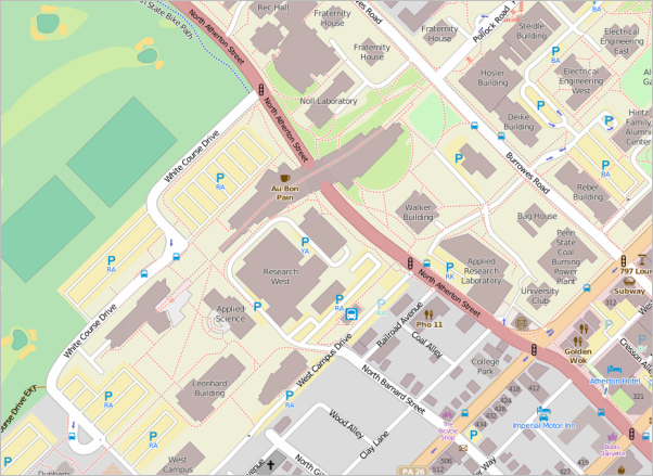
OSM originally gained popularity in places where government data was not freely available, but a thriving GIS community existed. For example, in the mid-2000s, the UK Ordnance Survey data was available only for purchase, and OSM grew rapidly as an attractive free alternative. In places where governments were willing to freely share their data, bulk upload negotiations were sometimes arranged. For example, the US has fairly thorough road coverage due to a US Census TIGER street data bulk upload.
OSM volunteer efforts constitute a social event and hobby for many, who gather for group data collection events known as "mapping parties." These activities organized armies of volunteers to walk, bike, and drive through sectors of a city with GPS units and notepads, returning later to a central lab to enter the data (Perkins and Dodge 2008). Although this is still useful in cases, nowadays, many OSM beginners can get pretty far just through tracing aerial photographs in simple browser-based editors. In addition to a physical exploration of the city, mapping parties now offer training, awareness, and renewed enthusiasm of OSM (Hristova et al. 2013).
How OSM features are contributed and tagged
To contribute a feature to OSM, you typically digitize a geometry (a point, line, or area) and then add descriptive attributes, or tags. For example, to tag a grocery store, you trace its building footprint and tag it with shop=supermarket. There's no restriction on the tags you can use, but the data is only useful to the degree that you tag things consistent with the way other OSM users have applied the tags.
To promote consistency in tagging, the OSM community has an informal tag voting and approval process organized on the OpenStreetMap wiki [235] site. Approved tags are added to the online documentation so that others can easily find and apply them. For example, the tag shop=supermarket [236] denotes a grocery store. Before you add a tag, check the wiki to make sure that you're using the established tag and syntax. If you create your own tag and start using it on many features, consider putting it through the OSM proposal process [237].
Benefits and weaknesses of OSM
OSM is not the only crowdsourced VGI project, but it is one of the most well known. As such, it provides a useful exemplification of the pros and cons of crowdsourcing and VGI.
Some of the main benefits of OSM include:
- There is no cost to use the data. In some locales, OSM may be the only freely available source of high-resolution GIS vector data. In other places, it may be the only source of data.
- The source data is available for download and use in derived cartographic products. Here, OSM differs from the crowdsourcing mechanism that Google Maps deployed, called Map Maker. Cartographers cannot download and re-use Google Map Maker data; whereas OSM is available to anyone with enough technical know-how to get the data.
- Because OSM allows people to add any type of feature, it may include a richer and more socially valuable set of features than commercial or government maps. Possibilities include trees, wheelchair ramps, food banks, spigots for potable water, and so forth.
- OSM data is flexible and can quickly be updated in the event that a new business opens, a bridge gets washed away, etc. In contrast, commercial and government maps tend to be updated on fixed cycles.
Some of the main challenges of OSM include:
- There is no systematic quality check performed on the data. You use the data at your own risk and should exercise care when using OSM information for mission-critical functions.
- The detail, precision, and accuracy of OSM coverage varies across space, without a simple means of detecting the variation. In the global South, some cities are missing basic street data, let alone other useful features such as parks, schools, and civic buildings. The Missing Maps [238] project, heavily promoted by the American Red Cross, is one organized effort attempting to address this situation.
- OSM is subject to contributor biases. Each contributor must make decisions about the types of features he or she will place on the map and the places he or she will map. Looking at the map of any given place on openstreetmap.org, we have little idea of who created the map and why. The browser-based tool Crowd Lens for OpenStreetMap [239] attempts to offer a window into the crowd that created OSM in a particular place. It shows that some places have garnered much more attention than others.
- The OSM community decides the types of features that are worthy of the community tagging system. This is accomplished through a semi-formal proposal and voting process which tends to reflect the interests of the contributors. In 2013, Stephens lamented that there were multiple tags for marking sexual entertainment venues in OSM, whereas proposals for tags denoting hospice services and daytime childcare had floundered. She attributed this directly to the fact that a significant majority of OSM contributors are male. Recent speakers at OSM conferences have raised attention to the consequences of gender and other imbalances in OSM, and have provided suggestions of how to make the OSM community more diverse [240].
- Unless you're just viewing the default map tiles, getting a focused set of data out of OSM often takes a lot more technical skill than getting the data in. Data ingress and retrieval techniques are covered in the lesson walkthrough and assignment, where you can judge this point for yourself.
Uses of OSM
The most basic use of OSM is to retrieve its map tiles as a background for other thematic layers. High-profile sites using OSM in this way include Foursquare, Craigslist, and Wikipedia. Some web developers switched to OSM as a basemap [241] after the Google Maps API introduced potential fees into its terms of service.
From a technical perspective, anyone can use a rendering engine like QGIS or Mapnik to draw tiles of OSM data. In fact, this is what you did with QGIS in the Lesson 5 walkthrough. The image below shows how you can select various basemap renderings on OpenStreetMap.org. Other companies such as Mapbox [242] have made their own OSM renderings that can be consumed as web services. In fact, Mapbox's business model has come to rely so heavily on OSM that the company has invested in near-real-time quality monitoring of incoming OSM edits by hosting OSMCha [243], an OSM Changeset Analyzer [244] tool originally written by Wille Marcel in 2015 (you need to sign in with a OSM account to be able to use the tool).
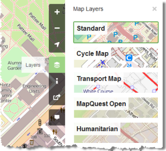
Let's now take a look at some of the ways OSM can be used "beyond the basemap."
Crisis response
OSM gained publicity as a disaster response aid in 2010 after the Haiti earthquake, as described in this PSU Geospatial Revolution video [245]. Prior to this disaster, publicly available digital data for Haiti was sparse, and OSM was limited to major roads and a handful of other features. In the weeks following the earthquake, Internet volunteers worldwide traced imagery and referenced out-of-copyright maps to create a detailed geographic database of the country in OSM. This provided helpful basemaps for humanitarian aid workers who were flocking to the country and needed maps to get around. It also served as an inventory of hospitals, churches, civic facilities, and other resources that could be used by responders.
The growth of OSM during this period was nothing short of dramatic, and a number of animations such as this video: OpenStreetMap - Project Haiti [246] have depicted the expansion of the map in Haiti during this time period. Zook et al (2010) offer an analysis of various methods of VGI and crowdsourcing used in the earthquake response, including OSM and the crisis mapping site Ushahidi.
Crowdsourced volunteer efforts work most efficiently when there is an organizing force behind the work. Using lessons from the Haiti experience, the Humanitarian OpenStreetMap Team [247] (HOT) now provides this function. After Typhoon Haiyan hit the Philippines in 2013, HOT provided tools to explain and partition the volunteer mapping work on OSM so that the most needed features and geographic areas were given priority. Volunteers visiting the HOT site could click a map sector to work on, and were given instruction about which features to trace and how to tag them. The image below shows the OSM Tasking Manager, an application used by HOT to catalog sectors completed and sectors that need work.
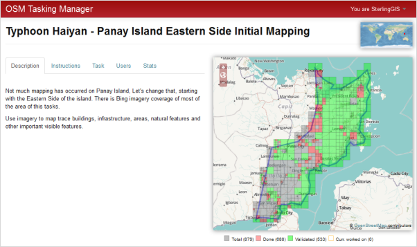
Providing a presence for unmapped or undermapped areas
The efforts to rapidly assemble crisis mappers in Haiti and the Philippines are admirable, but the ideal situation would be to already have the OSM data on hand. These regions only needed the mapping because sufficient information hadn't been contributed in the first place. Lack of technical infrastructure, a shortage of human and monetary capital, civil restrictions, and other factors can cause places to remain unmapped. Graham (2010) calls these places "virtual black holes" in VGI. Unfortunately, commercial Internet maps may also neglect these places if it is believed the search and advertising functions related to the map will not produce sufficient revenue to justify the investment.
OSM has been used as a way to give a presence to communities that have previously remained unmapped. Hagen (2010) describes a project in Nairobi wherein local youth volunteers were enlisted and trained to map the sprawling slum of Kibera. Home to hundreds of thousands of people, this settlement was little more than a name on previous maps. The Map Kibera [248] effort used OSM tools to record water points, toilets, clinics, schools, pharmacies, places of worship, and NGO offices. The result is a map that the residents can use to find local services and lobby the government for infrastructure support. The features added through this project are immediately apparent when you navigate to Kibera using even the default OSM map.
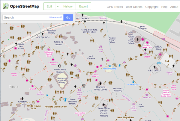
Similar stories can be found elsewhere in the world. When participants in a Buenos Aires hackathon wanted to map social services in a local slum, they found the area empty in commercial maps and decided to use OSM as a basemap [249]. Even when a street network exists, other layers such as bus routes may be helpful for individuals without automobiles, opening possibilities for local travel outside of daily routines. Motivated individuals have headed up an OSM project with bus routes in India [250], noting that a detailed local map can also help with tourism promotion efforts.
Thematic mapping for the social good
One of the advantages of OSM is its flexibility to store any type of feature, given the many tags that already exist and the community-based tag proposal and voting process. In some cases, specialized thematic maps have been created around a subset of feature types. Examples of these include:
- OpenCycleMap [251], specializing in drawing bicycle trails that people have submitted to OSM
- OpenSkiMap [252], showing ski lifts and trails
- Wheelmap [253], allowing the browsing and marking of wheelchair-accessible locations
- Philly Fresh Food Map [254], displaying urban farming resources and fresh food distribution outlets in Philadelphia, Pennsylvania. (This should look familiar!)
In these maps, OSM acts as a freely accessible repository for local knowledge of useful things. Some of these mapped features provide great value to a community, but are not monetarily lucrative and may be excluded from proprietary commercial maps. Even the default OSM tiles do not show all the above types of features because to do so would cause the map to be cluttered. There is a great need for developers who can retrieve custom subsets of data from OSM and display it in thematic maps.
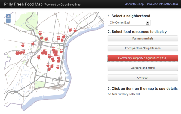
Remember that thematic maps are only possible because OSM allows free download and re-use of the data. Sites that use OSM for thematic mapping often rely on one of the various query APIs available for OSM, such as the Overpass API that allows the submission of custom tag queries through a web service. Asking a web service to give you all features matching a certain tag is often more manageable than downloading the entire OSM dataset for a region. You will get a taste of the Overpass API in the lesson walkthrough.
The maps and queries depend heavily on users maintaining consistency with established tag syntax. For example, the Philly Fresh Food Map relies on tags described in the Food Security [255] page of the OSM wiki.
References
- Graham, M. (2010). Neogeography and the palimpsests of place: Web 2.0 and the construction of a virtual earth.Tijdschrift Voor Economische En Sociale Geografie, 101(4), 422–436.
- Hagen, E. (2010). Putting Nairobi’s Slums on the Map. Development Outreach | World Bank Institute, 41 – 43.
- Hristova, D., Quattrone, G., Mashhadi, A., & Capra, L. (2013). The life of the party: Impact of social mapping in OpenStreetMap. In Proceedings of the AAAI International Conference on Weblogs and Social Media (ICWSM2013).
- Perkins, C., & Dodge, M. (2008). The potential of user-generated cartography: a case study of the OpenStreetMap project and Mapchester mapping party. North West Geography, 8(1), 19–32.
- Stephens, M. (2013). Gender and the geoweb: Divisions in the production of user-generated cartographic information. GeoJournal, 78(6), 1–16.
- Zook, M., Graham, M., Shelton, T., & Gorman, S. (2010). Volunteered geographic information and crowdsourcing disaster relief: a case study of the Haitian earthquake. World Medical & Health Policy, 2(2), 7–33.
Walkthrough: Getting source data from OpenStreetMap
Getting data out of OpenStreetMap (OSM) presents more technical challenges than putting data into OSM. When you put data into OSM, you can use your choice of a number of different types of editors. You can use any tags that you want, attempting to stick to tagging conventions of course.
In contrast, when you get data out of OSM, you have to deal with the following:
- Retrieving only the tags you need
- Retrieving the data format you need
- Not overwhelming yourself or the server by requesting too much data
Complicating matters is the fact that OSM returns data in its own structure of XML, which is not immediately readable by many GIS applications. Therefore, getting data from OSM often involves converting from this XML into some other format.
There are a variety of mechanisms for downloading OSM data. The easiest ones address the challenges by providing a way to filter the tags you want, allowing you to specify the output format, and allowing you to specify a geographic bounding box for the requested data, so you don't retrieve too much.
One of the most user-friendly GUI-oriented ways that I have found for retrieving OSM data is a server at BBBike.org [256]. This little web-based tool allows you to draw a bounding box interactively and specify the output format you want. After a while, you receive an e-mail with a link to download your data.
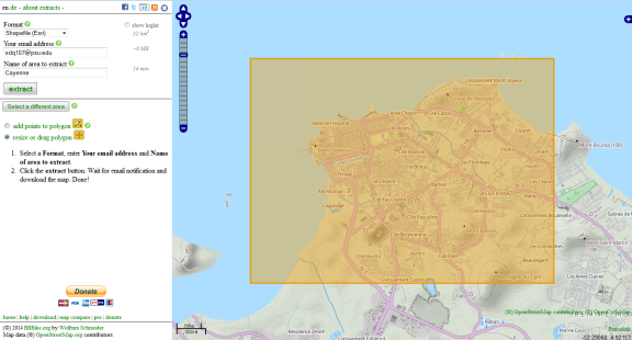
In the walkthrough, however, we'll use the OSM download mechanism that is available in QGIS via the OSMDownloader plugin. Although this way is a little more advanced than the BBBike extract service, it is more immediate and allows greater flexibility for the amount of data and tags selected.
Downloading OSM data using QGIS
Examine the image below of Cayenne, French Guiana. You'll notice that the city has detailed building footprint polygons available. Let's suppose that we want to get a shapefile of these building footprints using QGIS.
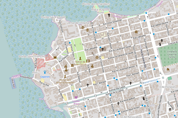
Note that we have defined our three pieces of essential information to filter the OSM data we want:
- The tags we want: any polygon with the building tag populated as anything other than building=no (a somewhat rare value but one that is occasionally used)
- The format we want: a shapefile
- The bounding box of data we want: just the city of Cayenne
While in a previous version of QGIS, downloading OSM data was integrated into the main program and available under Vector > OpenStreetMap > Download data, this functionality has been removed and now requires a plugin to be installed. On the positive side, these plugins now require much fewer steps to obtain the data. There are several plugins available that can be used for downloading OSM data. We here show you the steps using the OSMDownloader plugin. Go ahead and install this plugin from the QGIS plugin manager. You should be able to find it under "Not installed". When activated, the plugin will add a toolbar with a single button to QGIS:  When you click it, this button will become highlighted and you can then select an area in the map canvas for which you want to download the OSM data.
Now perform the following steps:
- Create a new data folder such as c:\data\Cayenne to download the data to.
- In QGIS start a new project and use EPSG:4326 for the coordinate reference system. This is just so that all coordinates displayed by QGIS will be WGS84 latitude and longitude coordinates.
- Add an OSM basemap to the project, then navigate to Cayenne in French Guiana at the northern coast of South America. The coordinates in the image below will help you if you have problems finding the city on the map.
- Activate the OSMDownloader button described in the previous paragraph, and then click and drag in the map canvas to select a rectangular area comprising the city. This opens the OSMDownloader dialog box shown below. If you want to use exactly the same area we use here, manually edit the upper and lower boundaries for the latitude and longitude coordinates to be the same as in the screenshot.

Figure 9.8 -
Under Save Location, press the Save File button and navigate to the folder you created in step 1. Then use cayenne.osm for the file name.
-
Click OK, which will start the download process. A progress bar will appear and finally a window informing you that the download has finished.
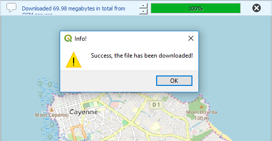
Figure 9.9 -
We are done using the download plugin now. Next, let's add the downloaded .osm file with the OSM data to our QGIS project. For this, you can simply drag the cayenne.osm file from the Windows File Explorer onto the map canvas in QGIS. The .osm file contains entities of different geometry type. However, the layer that will be added to QGIS can only contain features of a single geometry type. Therefore, you will be shown a dialog window in which you have to pick that geometry type. Since we are interested in building polygons, you should select "multipolygons" here and then click the button either called OK or Add Layers.
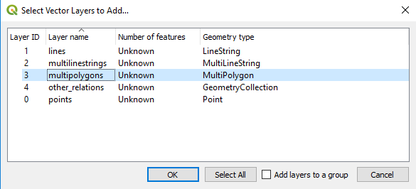
Figure 9.10 - You should see a new layer called cayenne_multipolygons appear in your QGIS project as shown in the image below.
Now you just need to select only the building polygons from this layer.
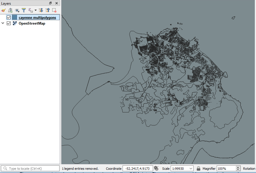 Figure 9.11
 - In the map table of contents, right-click cayenne_polygons and click Open Attribute Table. Have a quick look at the attribute table and check out the building column. This is what we will refer to in our query to filter the layer.
- At the top of the attribute table, click the Select features using an expression
 button.
 - Paste the following query into the Expression box, including all quote marks: "building" != 'NULL' AND "building" != 'no'
This expression filters out everything that's not a building. When you do this with your own data of interest, you'll need to create some expression that selects only the tag combinations that you want.
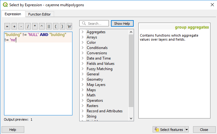 Figure 9.12
 - Click Select features. You should see the building features selected in the map.
- In the map table of contents, right-click the cayenne_polygons layer and click Export -> Save Features as....
- Choose Esri shapefile as the format and specify an output location. Select the Save only selected features option. Then click OK. (The "Add saved file to map" option will most likely appear at the very bottom of the window but should already be enabled by default.)
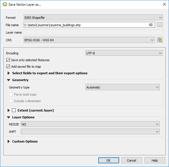 Figure 9.13
 - Use QGIS to verify that your exported shapefile contains only the buildings.
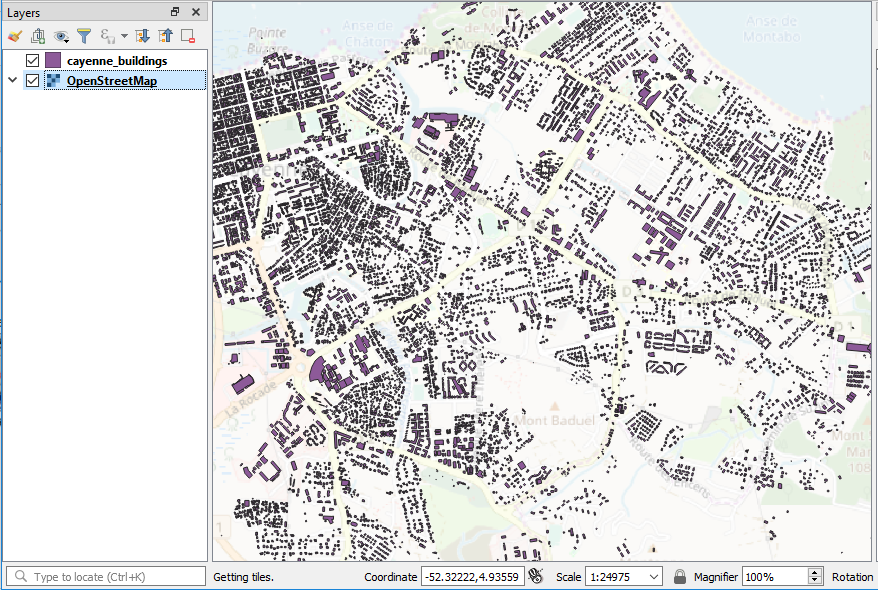 Figure 9.14
Downloading data using the Overpass OpenStreetMap query API
Behind any data retrieval mechanism from OSM is a web service request. You can send these requests directly from your web browser or an automated program using an OSM query API. One of the most powerful of these APIs is called Overpass [257]. Try the following:
- Paste the following URL in a web browser:
http://www.overpass-api.de/api/xapi_meta?*[building=yes][bbox=-52.35,4.88,-52.25,4.98]
Notice what this is requesting...It should look familiar. - When prompted to save the file, save it as buildings.osm. It's possible that your browser will directly download and save the file under the name xapi_meta rather than asking you for a name. Therefore, if nothing happens, check your Downloads folder, and if you see the file, rename it to buildings.osm.
- Open buildings.osm in a text editor and see what all the buildings in Cayenne look like when expressed as OSM-formatted XML.
You can use Python or other scripting languages to make these requests automatically. For example, here's how you could use Python to query OSM for all the farmers' markets in Philadelphia and save them to a .osm file. (You're not required to run this code).
import urllib

workspace = "C:\\data\\OSMdev\\"

# Make data queries to jXAPI
marketsXml = urllib.urlopen("http://www.overpass-api.de/api/xapi_meta?*%5Bshop=farm%5D%5Bbbox=-75.29,39.86,-74.95,40.15%5D").read()

# Make farmers markets file
marketsPath = workspace + "markets.osm"
marketsFile = open(marketsPath, 'w')
marketsFile.write(marketsXml)
marketsFile.close()
For Python junkies: The above code uses a library called urllib which is able to make web requests and read the responses. You just have to provide the URL for the request. So as not to be interpreted as defining a list, the "[" and "]" characters are escaped using the %5B and %5D sequences, respectively, but otherwise the query has the same syntax as the one you issued above for Cayenne buildings. The resulting XML is then written to a file using the standard Python write method.
A script like this might be useful if you wanted to update one or more datasets on a periodic basis. The script could be combined with GDAL processing to get the data into a format suitable for your web map. Recent versions of GDAL (1.10 and later) can read OSM XML and convert it to different formats, such as GeoJSON or shapefiles. (Be careful with shapefiles though, because GDAL plops most of the less common "other tags" into one field that gets cut off at 256 characters, a limitation of the shapefile format).
As an exclamation point at the end of all this geekiness, play around with the graphical tool overpass turbo [258] for a few minutes. This gives you an interactive environment for querying OSM and seeing the results on the map. You can save any interesting result in popular formats, such as KML. This is helpful if you just want to make a one-off query to OSM for some particular feature type.
There are many circumstances and needs that can affect the way you retrieve data from OSM. Hopefully, this walkthrough has provided enough options that you can make an informed decision about how to best get the scope and scale of data you need. Now let's go to the lesson assignment, where you'll get some experience with the other side of things: putting data into OSM.
Lesson 9 assignment: Evaluate OpenStreetMap usage and contribute to OpenStreetMap
The Lesson 9 assignment has two parts: reporting on a web map that uses OpenStreetMap (OSM), and actually editing OSM yourself. You will produce a single document describing these efforts.
Reporting on a web map that uses OSM
Find an Internet map that uses some element of OSM. Produce a write up of several paragraphs describing the following:
-
What is the purpose and URL of the site, and who built it?
-
How is OSM being used? (i.e., Is the site simply pulling the OSM tiles, or is the source data used for creating thematic layers, etc.?)
-
Include at least one screenshot showing the OSM data.
-
-
What advantages and disadvantages are introduced into this map by using OSM data?
-
Do you see any other appropriate ways that OSM data could be used in this site?
Editing OSM yourself
In this part of the assignment, you'll get some practice with adding data to OSM in your town or some other place that you know well. You'll take some "before" and "after" screenshots to demonstrate the things you added to the map.
The easiest way to get started with editing OSM is using the in-browser editor at OpenStreetMap.org [31], which is called iD.
- Visit OpenStreetMap.org [31] and register for an account. This requires creating a name and password and supplying your e-mail address (so you can prove you're a person and not a robot).
- After you've created the account, return to OpenStreetMap.org and log in. Do not use Internet Explorer for this part of the exercise, because it cannot display the iD editor.
- Navigate to your hometown or another place you want to edit and click the Edit dropdown button. If asked which editor you want to use, choose iD.
- Click Start the Walkthrough and carefully follow all instructions to complete the iD training.
ID includes a walkthrough for beginners that gives you some hands-on practice with tracing and tagging features. Thus, full editing instructions for using iD are not included in this lesson. Follow the walkthrough, and you should have the basics down. - After completing the walkthrough, scan the features available in your hometown and identify some things you want to add. The easiest way to start is probably by tracing a building. Choose to create an Area and trace around a building that you see in the imagery.
The first thing to do is tag it with building=yes. Also, if the building has a name, supply the name tag.
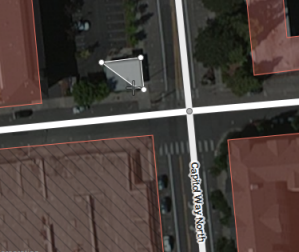 Figure 9.15Now you can provide other tags further specifying the purpose of the building, if these are known. An appropriate tag to add in the above image might be amenity=restaurant.
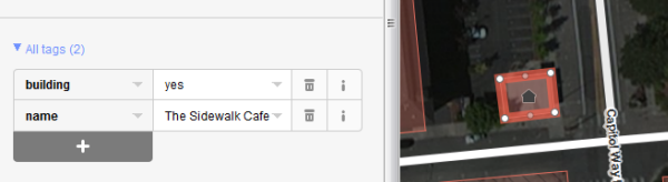 Figure 9.16
You can optionally supply addresses for features, but this involves several OSM tags. The easiest way to do it in iD is to fill in the Address form. This ensures all the address parts get the correct tags.Adding addresses is not required for this assignment.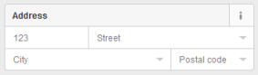 Figure 9.17
 - Continue with your assignment by adding (or modifying) a total of at least 7 features, making sure the following criteria are satisfied:
- Five different types of features must be represented. In other words, don't just trace 7 building footprints. Use the OpenStreetMap wiki to learn the correct way to tag different types of features. You can also use the left-hand Search menu in iD to get hints about tags, but, during this assignment, you should verify that the tags placed by iD match what you intended to map as described in the OpenStreetMap wiki documentation.
- Point, Line, and Area features must be represented. You can satisfy this requirement by adding new lines or adjusting existing lines. For example, sometimes roads need more detail to produce smooth curves, line up with the imagery, etc.
- Before you add the features, go to the main OSM page at OpenStreetMap.org and take some screen captures.
If you have trouble thinking of what to add, consider mapping parks, schools, churches, restaurants, civic buildings, clinics, ponds, wetlands, etc. New subdivisions are also a great opportunity for mapping roads. You can get more ideas by looking around OSM in a city that's been mapped in detail, such as Seattle or State College. Another way to get good ideas is by walking or biking around your town.
- Produce a list of the features you edited and add it to your report that you created in the first part of the project. Include a list of all tags that you placed or edited on each feature. These tags must comply with the community-approved documentation on the OpenStreetMap wiki. Link for your reference here: https://wiki.openstreetmap.org/wiki/Map_features [259]
- Wait for about 10-15 minutes after your edit session and then go to OpenStreetMap.org and take some screen captures of the new features. Note that OSM updates their tile levels at different times, so your feature may only be visible at certain tile levels. Choose any tile level that works for the screenshot. You don't have to supply 7 screenshots; just provide enough to show some of the "before" and "after" effects of your edits.
- Paste the screenshots in your report.
Deliverable
Submit a single document containing the two assignment parts above to the Lesson 9 assignment drop box on Canvas.Lesson 10: Course wrapup and term project submission
The links below provide an outline of the material for this lesson. Be sure to carefully read through the entire lesson before returning to Canvas to submit your assignments.
Note: You can print the entire lesson by clicking on the "Print" link above.
Overview
Take a moment and look back at how far you've come. In this course, you've learned what free and open source software (FOSS) is and how it fits into the practice of web mapping. You've also learned how to take raw GIS data, process it, assemble it into beautiful maps, expose it as web services, and present it as a finished product in an interactive web map.
As a demonstration of these skills, you are expected to submit a term project that exposes some theme of interest to you as a web map. You have already started creating the pieces of this project in some of your weekly lesson assignments, and a portion of this final week of the course is reserved for you to solely focus on completing the project.
After the projects are submitted, we will have a "mini-conference" where you'll get the chance to browse other students' work and review it. This may provide ideas and feedback for your future web mapping projects.
Checklist
- By the end of Sunday (three days before the course end date), submit your term project video as described on the term project submission page [260].
- Between Monday and Wednesday (during the last four days of the course), review at least two videos.
- By the end of Wednesday (the course end date), post your term project write-up to the drop box on Canvas.
- By the end of Wednesday (the course end date), complete the Student Educational Experience Questionnaire on Canvas
Term project submission guidelines
In Geog 585, you are expected to create a term project that takes some data of interest to you and fuses it into a useful web map. The term project can be simple and focused in nature, but must include:
- a basemap to give geographic context;
- one or more thematic layers that are separate from the basemap;
- one or more interactive elements that reveal more information (such as being able to click a feature to see a list of attributes, or selectively filter information in a map layer).
In creating your term project, you should use at least one tool or technique that was not covered in the course materials. This could, for instance, be a tool for (pre)processing the data, or it could be a Leaflet class or method that you explored. You don't have to know this part when you make the proposal, but as you work through the different exercises in the course, you should stay aware of additional functions you could incorporate to meet this requirement.
The project must be built entirely with FOSS. This requirement is not in place to make you a FOSS "purist"; rather, it is intended to compel you to fully practice the skills you have learned in this course and discover new ways of doing things. If there's some piece of your project data processing that you don't think can be completed with FOSS, please discuss it with the instructor.
There are three parts to the term project submission:
- an online video demonstrating the project functionality.
- a write-up describing the project purpose and approach. This also includes your code.
- two brief reviews of other students' projects.
The requirements of the submission are described in detail below. Please see the term project grading rubric on Canvas to understand exactly how these requirements will be evaluated.
Project video submission
To share your project with the instructor and others, you will create an online screen recording "video" explaining the purpose of the project and giving a tour of its functionality. In under 5 minutes the video must cover the following:
- Give an overview of the purpose of the project and how a user would get benefit out of this map.
- Explain where you got the data.
- Describe the preprocessing steps and tools you employed in preparing the data for web map use.
- Demonstrate how the data is divided into basemap and thematic layers.
- Describe the approaches you took for exposing the data as web services and why you chose those approaches (e.g., dynamically drawn service using WMS, tiles designed with QGIS, tiles pulled from OpenStreetMap, GeoJSON layer drawn by the browser, etc.).
- Demonstrate the interactive elements in your web map. Follow the "story" of what a user would do when approaching your map. For example: "Suppose that you are working for _____ and you want to learn ____, so you come to this map and see that you can turn on layer ______ which tells you _______. You then see that ______ is clickable, so you click it and learn that _______ is ________. You now know _________, which helps you make a decision about _______."
- Describe at least one tool or technique used in the creation of your web map that was not covered in the course materials. This tool or technique should be something different than the GDAL/OGR command you described in homework assignment 3, part2, but it can be related to your FOSS review from homework assignment 8.
It is expected that the video will just record the screen (you don't need to appear on camera). There are many alternatives to produce the video, including free screen recording software and services. As Penn State students, you have free access to Kaltura [261]. Another free option that worked well in the past is Screencast-O-Matic [262]which requires you to run a small program on your computer. The recorded video can be stored as a .mp4 file, or it can be shared via their web site. Alternatively, if you have access to professional screen recording software such as Captivate, Camtasia, Fraps, etc., you may use it. Much of this software is available for free trial periods. An option for Mac users is to use QuickTime; there are descriptions of how to do this out there on the web. For sharing your video, you can also upload it to any other file sharing service, for instance, dropbox.com, GoogleDrive, or OneDrive.
It's strongly recommended that you reserve at least a day or two for creation of the video. This will allow you to accommodate any unforeseen technical challenges and do multiple "takes" if necessary. Things will go more smoothly if you prepare a script or outline of things you want to show, and refer to this during the video recording.
The video is due Sunday evening before the course end date. To submit the video, follow the description on the Term project submission and mini conference page [260].
Project writeup and code submission
Please also submit a 500+ word writeup recapping:
- the purpose of your project;
- the decision process you went through when deciding how to serve the different layers;
- the ways that your project reinforces and extends the information in the Geog 585 lessons;
- the things you learned in this project that will be most valuable to you in your professional or academic career.
Please submit all the source code for your project together with your writeup. Please zip the original HTML, JavaScript, and all other files required by your project together. Do not copy & paste the code into your writeup. Optional: If you host your final term project map in your AWS S3 storage as in homework assignment 7, please include the public S3 URL for your main .html file in your write-up. That will then allow us to directly test out your final web map application.
The writeup should follow professional writing and grammar conventions and should be spell checked. The writeup and code are due in the term project drop box by the course end date.
Tip: If you complete the writeup before you do your video narration, the words may come more easily when you are "on camera".
Reviews of other students' projects
The project will no doubt be a learning experience for you, but there is also plenty to learn from other students' experiences and submissions. During the final three days of the course (Monday, Tuesday, Wednesday), take some time on the "Term project video & review forum" on Canvas to browse other submissions. Select two projects of interest to you and, with each, post a brief review as a reply. Your review should include:
- strengths that you see in the person's submission;
- elements that might be improved in the person's submission using information we covered in Geog 585 or other tools you discovered during the course;
- comments on ways that the project might be applied to other disciplines or real-world problems.
These reviews are due by the course end date.
Term project submission and mini conference page
Academics often attend conferences where they share their discoveries and browse the work of others to gain new ideas and offer feedback. Although we can't all physically meet together, the "Term project video & review forum" on Canvas will serve as our virtual conference location where you can get the same benefits.
By the final Sunday evening of the course, make a post in that forum containing a link to your term project video. Then, by the course end date, please reply to at least two other students' videos in that forum. See the Term project submission guidelines for further instructions about how to make these submissions.