Spatial Interpolation

The Basic Concept

A key idea in statistics is estimation. A better word for it (but don't tell any statisticians I said this...) might be guesstimation, and a basic premise of much estimation theory is that the best guess for the value of an unknown case, based on available data about similar cases, is the mean value of the measurement for those similar cases.

This is not a completely abstract idea: in fact, it is an idea we apply regularly in everyday life.

I'm reminded when a package is delivered to my home. When I take a box from the mail carrier, I am prepared for the weight of the package based on the size of the box. If the package is much heavier than is typical for a box of that size, I am surprised, and have to adjust my stance to cope with the weight. If the package is a lot lighter than I expected, then I am in danger of throwing it across the room! More often than not, my best guess based on the dimensions of the package works out to be a pretty good guess.

So, the mean value is often a good estimate or 'predictor' of an unknown quantity.

Introducing Space

However, in spatial analysis, we usually hope to do better than that, because of a couple of things:

1. Near things tend to be more alike than distant things (this is spatial autocorrelation at work), and
2. We have information on the spatial location of our observations.

Combining these two observations is the basis for all the interpolation methods described in this section. Instead of using simple means as our predictor for the value of some phenomenon at an unsampled location, we use a variety of locally determined spatial means, as outlined in the text.

In fact, not all of the methods described are used all that often. By far, the most commonly used in contemporary GIS is an inverse-distance weighted spatial mean.

Limitations

It is important to understand that all of the methods described here share one fundamental limitation, mentioned in the text but not emphasized. This is that they cannot predict a value beyond the range of the sample data. This means that the most extreme values in any map produced from sample data will be values already in the sample data, and not values at unmeasured locations. It is easy to see this by looking at Figure 6.1, which has been calculated using a simple average of the nearest five observations to interpolate values.

Figure 6.1: The results of a moving average interpolation process (red line) compared to the sample of five nearest points (black dots). The red line is the interpolated value (i.e., vertical position) based on a simple average of the nearest five sample values.

Credit: O'Sullivan

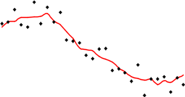
It is apparent that the red line representing the interpolated values is less extreme than any of the sample values represented by the point symbols. This is a strong assumption made by simple interpolation methods that kriging attempts to address (see later in this lesson).

Distinction Between Interpolation and Kernel Density Estimation

It is easy to get interpolation and density estimation confused and, in some cases, the mathematics used is very similar, adding to the confusion.