With even a basic appreciation of regression (Lesson 5), the idea behind trend surface is very clear. Treat the observations (temperature, height, rainfall, population density, whatever they might be) as the dependent variable in a regression model that uses spatial coordinates as its independent variables.
This is a little more complex than simple regression, but only just. Instead of finding an equation
where z are the observations of the dependent variable, and x is the independent variable, we find an equation
where z is the observational data, and x and y are the geographic coordinates of locations where the observations are made. This equation defines a plane of "best fit."
In fact, trend surface analysis finds the underlying first-order trend in a spatial dataset (hence the name).
As an example of the method, Figure 6.2 shows the settlement dates for a number of towns in Pennsylvania as vertical lines such that longer lines represent later settlement. The general trend of early settlement in the southeast of the state around Philadelphia to later settlement heading north and westwards is evident.
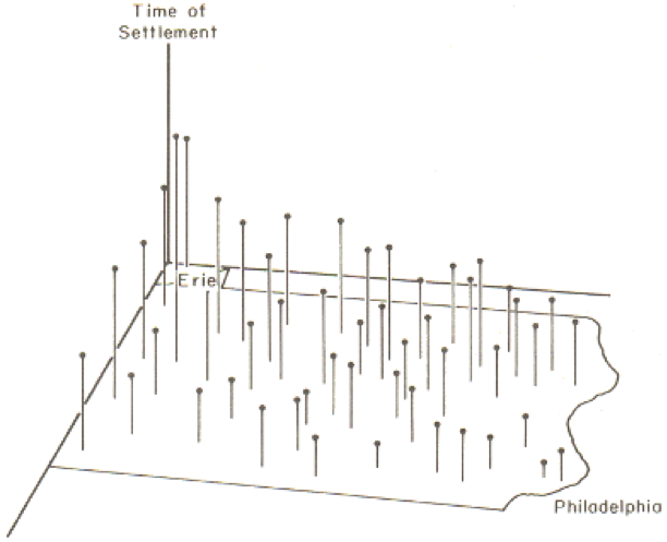
In this case, latitude and longitude are the x and y variables, and time of settlement is the z variable.
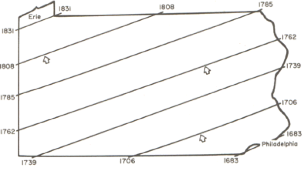
When trend surface analysis is conducted on this dataset, we obtain an upward sloping mean time of settlement surface that clearly reflects the evident trend, and we can draw isolines (contour lines) of the mean settlement date (Figure 6.3).
While this confirms the evident trend in the data, it is also useful to look at departures from the trend surface, which, in regression analysis are called residuals or errors (Figure 6.4).
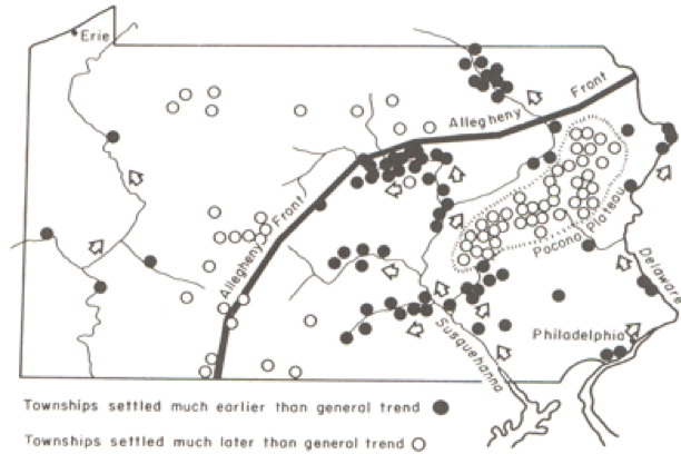
The role of the physical geography of the state on settlement time is evident in the pattern of early and late settlement, where most of the early settlement dates are along the Susquehanna River valley, and many of the late settlements are beyond the ridge line of the Allegheny Front.
This is a relatively unusual application of trend surface analysis. It is much more commonly used as a step in universal kriging, when it is used to remove the first order trend from data, so that the kriging procedure can be used to model the second order spatial structure of the data.