3.5 The Skew-T Diagram: A Wonderful Tool!

3.5 The Skew-T Diagram: A Wonderful Tool!

The skew-T vs –lnp diagram, often referred to as the skew-T diagram, is widely used in meteorology to examine the vertical structure of the atmosphere as well as to determine which processes are likely to happen.

You may know a little about the skew-T from previous study, but for those who did not take a previous course or who need a refresher, there are many useful websites that can help you understand the skew-T and how to use it. Two useful resources are the following:

Weatherprediction.com Review of Skew-T Parameters

Introduction to Mastering the Skew-T Diagram Video

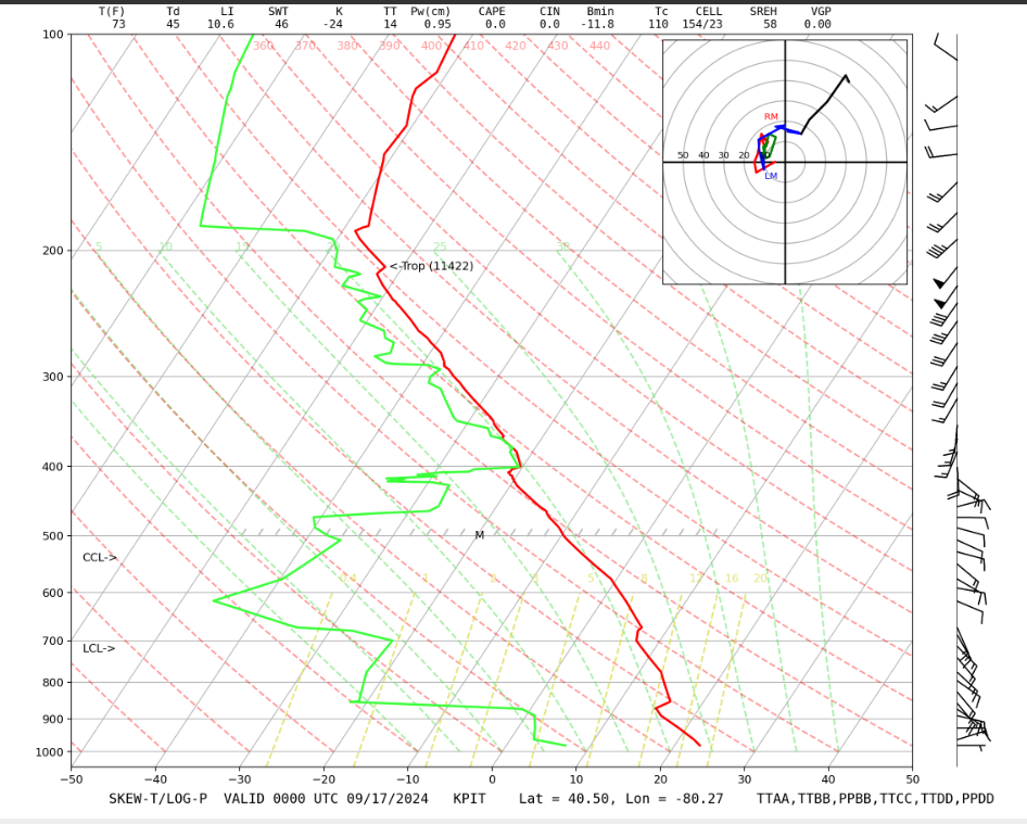
First, familiarize yourself with all of the lines. Look at a radiosonde ascent, such as the one from the National Center for Atmospheric Research Research Applications Laboratory (type of plot: GIF of skew-T). The atmospheric sounding lines are temperature (solid red line) and dewpoint temperature (solid green line). These lines are plotted on a grid that shows –lnp on the vertical axis (horizontal blue lines) and temperature on the horizontal axis (blue lines tilting up and to the right—which is where "skew" comes from). –lnp is used because it varies nearly linear with height and the skewing of the temperature lines allows soundings to be shown without going out of bounds of the graph.

Here is a blank skew-T diagram that you can play with and practice on. The diagram has an electronic pen that allows you to draw on it. This diagram will be used in Practice Quiz 3-4 and Quiz 3-4, so become familiar with it.

The most recent Skew-T Log-P diagram created from the radiosonde launched from Pittsburgh, PA. The date can be seen in the bottom left, and the time is in UTC time.

Credit: National Center for Atmospheric Research (NCAR) (Public Domain)

Please also note the following:

• The dry adiabat is the same line as an isentrope (curved red dash lines tilting to the upper left).
• The water vapor mixing ratio is the saturation water vapor mixing ratio at the dewpoint temperature, T_d, for each pressure level (gold dot-dash lines tilting to the upper right).
• In clear air, for air parcels moving vertically:
  • air parcels move along the dry adiabat and the potential temperature remains constant, even if they contain moisture;
  • the water vapor mixing ratio is constant (but notice that T_d changes!);
  • T_d of an air parcel moving vertically (and adiabatically) is decreasing, but not as fast as T of that air parcel is decreasing.
• Eventually, an air parcel moving vertically (along the dry adiabat) will have a temperature and dewpoint temperature that are the same, thus saturated.
• At this altitude level, called the Lifting Condensation Level (LCL), the relative humidity = 100%, T = T_d, w = w_s, and e = e_s. At this pressure and temperature, a cloud forms. Actually, the formation of a cloud requires a relative humidity that exceeds 100% by a few tenths of a percent, but we generally use 100% for the skew-T calculations. We will see why this extra relative humidity is necessary in the next lesson.

See the video below (1:19) for further explanation:

Moist Adiabat

When the air parcel is in a cloud, ascent causes a temperature decrease while the air remains saturated (i.e., w = w­_s, RH = 100%). Since w_s decreases, the amount of water in the vapor phase decreases while the amount in the liquid or solid phase increases, but the total amount of water is constant (unless it rains!). As water vapor condenses, energy is released into the air and warms it a little bit. Thus, the lapse rate of the moist adiabat (curved dot-long-dash green lines tilting toward the upper left) is less than the lapse rate of the dry adiabat (9.8 K/km).

As long as it doesn’t rain or snow, an air parcel will move up and down a moist adiabat as long as it is in a cloud and will move up and down a dry adiabat when w < w_s below the LCL.

• Once a cloud forms, any further rise of the air parcel will follow the moist adiabat (condensation of water vapor heats the air so that the temperature decrease with height is less than that of the dry adiabat). As long as the ascent is in the cloud, the relative humidity will remain near 100% and w = w_s(T). Since T decreases on ascent, w_s decreases, and more water goes into the liquid or ice phase.
• If the air parcel, containing the liquid or ice that was formed, descends, it will move along the moist adiabat until it again reaches the LCL, at which point all of the liquid water or ice will have evaporated or sublimed. Just below the LCL, all of the water will be vapor and the air parcel will descend along the dry adiabat and the water vapor mixing ratio will be constant.

The following is a summary for air parcel ascent and descent:

• From the initial p, T, and T_d (or w), locate two points on the skew-T: (1) p and T and (2) p and T_d (or w).
• Starting at the first point, move the parcel up the dry adiabat.
• Starting at the second point, move the parcel up the constant-w line. Note that T_d is continually changing, so use w.
• Where the two lines intersect is the LCL.
• A cloud will form.

• If the air parcel continues to rise inside the cloud,
  • w will always equal w_s.
  • the air parcel will follow the moist adiabat.

• If the parcel then descends,
  • it will follow the moist adiabat down to the LCL.
  • it will follow the dry adiabat below that.
  • w will follow the w line below that.

The following video (1:43) discusses the process of adiabatic cooling and heating.

Other Potential Temperatures

There are other potential temperatures that are useful because they are conserved in certain situations and therefore can help you understand what the atmosphere is doing and what an air parcel is likely to do.

Virtual Potential Temperature

Virtual potential temperature is the potential temperature of virtual temperature, where density differences caused by water vapor are taken into account in the virtual temperature by figuring out the temperature of dry air that would have the same density:

This quantity is useful when comparing the potential temperatures (and thus densities) of air parcels at different pressures.

Wet Bulb Potential Temperature

The wet-bulb temperature is the temperature a volume of air would have if it were cooled adiabatically while maintaining saturation by liquid water; all the latent heat is supplied by the air parcel so that the air parcel temperature, when it descends to 1000 hPa, is less than its temperature would be had it descended down the dry adiabat.

The wet bulb temperature at any given pressure level is found by finding the LCL and then bringing the parcel up or down to the desired pressure level on the moist adiabat.

The wet bulb potential temperature, Θ_w, is the wet bulb temperature at p = 1000 hPa. 

How can we use the wet bulb potential temperature? The wet bulb potential temperature is conserved, meaning it does not change, when an air mass undergoes an adiabatic process, such as adiabatic uplift or descent. If we consider large air masses that acquire similar temperature and humidity, then this entire air mass can take on the same wet bulb potential temperature. Colder, drier air masses will have a lower Θ_w. The Θ_w of this air mass can change if a diabatic process occurs, such as the warming of a cold air mass as it moves over warmer land, or the cooling of an air mass by radiating to space during the night, but these processes can sometimes take days. So an 850-mb map of Θ_w is one indicator of air masses and the fronts between air masses. 

See the video below (:32) for further explanation:

Equivalent Potential Temperature

The equivalent potential temperature is the temperature that an air parcel would have if it were lifted adiabatically until all of the vapor were condensed and removed, and then brought to 1000 hPa adiabatically. For example, let's say you have an air parcel with some water vapor in it below the LCL. To find the equivalent potential temperature, you would (1) lift the parcel to the LCL along a dry adiabat, (2) lift the parcel along the moist adiabat all the way to the stratosphere so that all the water vapor condensed into liquid, and (3) bring the parcel down to 1000 hPa along the dry adiabat. Equivalent potential temperature accounts for the effects of condensation or evaporation on the change in the air parcel temperature.

Every 1 g/kg (g water vapor to kg of dry air) causes Θ_e to increase about 2.5 K. So, a moist air parcel with w = 10 g kg^-1, which is not uncommon, will have Θ_e that is 25 K greater than Θ.

Approximately,

where Θ is the potential temperature, l_v is the latent heat of vaporization, w is the water vapor mixing ratio, and c_p is the specific heat capacity at constant pressure.

How can we use the equivalent potential temperature? The equivalent potential temperature, Θ_e is conserved when an air parcel or air mass undergoes an adiabatic process, just like the wet bulb potential temperature, Θ_w, is. Note also the total amount of water in vapor, liquid, and ice form is also conserved during adiabatic processes. The total amount of water is quantified using the total water mixing ratio, w_t, which is defined in the same way that the water vapor mixing ratio (w) is defined except that it also includes liquid and solid water in the numerator. So, if we look at Θ_e and w_t, we can learn a lot about the history of an air parcel. These conserved quantities are very useful to understand the history of air parcels around clouds. For example, if Θ_e changes but w_t is constant, then the air parcel was either heated or cooled by a non-adiabatic process. On the other hand, if both Θ_e and w_t change proportionally, then two air parcels with different initial values for Θ_e and w_t have mixed. On a larger, more synoptic scale, gradients in Θ_e can be used to indicate the presence of fronts. 

Another use of Θ_e is as an indicator of unstable air. Air parcels that have higher Θ_e tend to be unstable. Thus regions of high-Θ_e air are regions where thunderstorms might form if the surface heating is great enough to erase a temperature inversion. 

See the video (1:01) below for further explanation: