Prioritize...
Once you have finished this section, you should be able to create a Hovmöller diagram in R.
Read...
For this example, we are going to recreate the original Hovmöller diagram using reanalysis output. To follow along, download this dataset of 4X daily geopotential heights from the NOAA 20th Century Reanalysis. To read more about the reanalysis, check out this link.
Define the Problem
We begin by defining the problem. Since we are recreating a diagram, the problem is already defined. We want to look at the evolution of troughs and ridges. This means we need to look at the time aspect and the longitudinal aspect (as waves generally progress west to east).
Select Variables and Dimensions
We are going to look at the 500-mb geopotential heights. Since we want to know the time evolution across longitudes, the dimensions will be time (y-axis) and longitude (x-axis). This means we need to average over latitude. Specifically, I will average over 35°N to 60°N (consistent with the original diagram and reflective of the mid-latitude jet stream region).
Prepare Data
We begin by loading in the data. This is a NetCDF file, so you need to use one of the many packages that will open it. My favorite is ‘RNetCDF’.
Your script should look something like this:
# install and load RNetCDF
install.packages("RNetCDF")
library("RNetCDF")

# load in 20CR monthly temperature
fid <- open.nc(“NOAA_20CR_dailyHeights.nc")
data20CR <- read.nc(fid)
The data frame contains the pressure levels for the vertical profile (level), latitudes (lat), longitudes (lon), time (time), and the geopotential heights (hgt-units meters). You can use the ‘print.nc’ command to read more about the file. The starting time is January 1st, 1945 and the ending time is December 31st, 1945. Each day has 4 observations.
The geopotential height has 4 dimensions (lonXlatXlevelsXtime). For the first step, I need to select out the 500-mb level. To do this, we need to determine the index of the 500-mb pressure.
Your script should look something like this:
# extract out pressure level
presLev <- which(data20CR$level==500)
Now, extract out the heights.
Your script should look something like this:
# extract out 500 height
hgt500 <- data20CR$hgt[,,presLev,]
We will plot time on the y-axis and longitude on the x-axis. This means we need to do something about the latitudes. Similar to the original, we will average over 35oN to 60oN. Start by extracting the latitude bounds.
Your script should look something like this:
# create latitude index
latIndex <- which(data20CR$lat < 61 & data20CR$lat > 34)
Now we average over this latitude range for every timestamp and every longitude. We will do this by using the ‘apply’ function.
Your script should look something like this:
# average over latitude index
LatAveHgt500<- apply(hgt500[,latIndex,],c(1,3),mean)
Now we have a variable with dimensions’ longitude by time. But the time is for the whole year, and I want to only extract out the November values. Let’s create a valid time index and then extract out the heights.
Your script should look something like this:
# time is in hours since 1800-1-1 00:00:0.0
time <- as.Date(data20CR$time/24,origin="1800-01-01")

# create a time index for November
timeIndex <- which(format(time,'%m')==11)

# Extract out heights for time period
tempHgt500 <- LatAveHgt500[,timeIndex]
Now we are left with a variable that has 2 dimensions (longitude and time) over our desired time period at our desired pressure level. We can finally plot the data.
Plot Hovmöller
For this example, I will use the function ‘filled.contour’. Let’s give it a try. Run the code below.
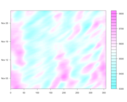
There are a few issues with this plot. For starters, the longitude values are not displayed in an intuitive manner. Second, to emulate the original plot, we should reverse the time so the starting date (November 1st) is at the top.
To fix the longitudes, we need to move the second half (180-360) to the front. This will create the 180 W (-180) to 180 E (+180) values similar to the original.
Your script should look something like this:
# determine half way point
halfLon <- length(data20CR$lon)/2

# change longitude order
finalLon <- c(data20CR$lon[(halfLon+1):length(data20CR$lon)]-360,data20CR$lon[1:halfLon])

# Change the matrix to match longitude
finalHgt500 <- matrix(NA,dim(tempHgt500)[1],dim(tempHgt500)[2])
finalHgt500[1:halfLon,] <- tempHgt500[(halfLon+1):length(finalLon),]
finalHgt500[(halfLon+1):length(finalLon),]<- tempHgt500[1:halfLon,]
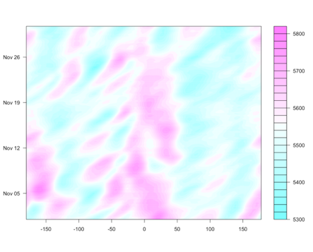
The code above first determines the halfway point with the longitudes. Then the code changes the longitude values to make them -180 to 180 or 180W to 180E. Finally, the code changes the matrix to match this switch in longitude. Let’s plot to confirm we made the correct changes. Run the code below:
Below is a larger version of the figure:
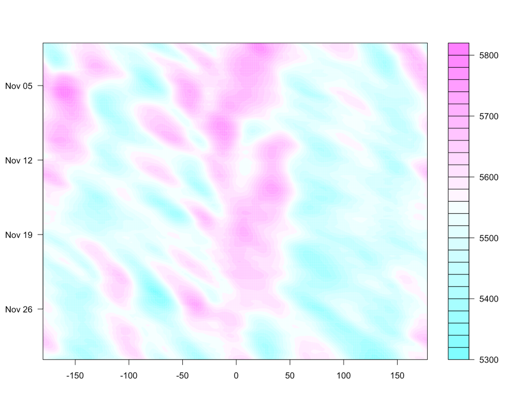
Now, let’s fix the time aspect. We can reverse this within the ‘filled.contour’ function by using the ‘ylim’ parameter. Run the code below:
Below is a larger version of the figure:
Now, let’s work on making this figure look nicer. First, let’s change the unit to decameters (consistent with the original). Run the code below:
Below is a larger version of the figure:
One thing to note, the range of the geopotential height is different compared to the original. This is a different dataset, and we would not expect them to be exactly the same.
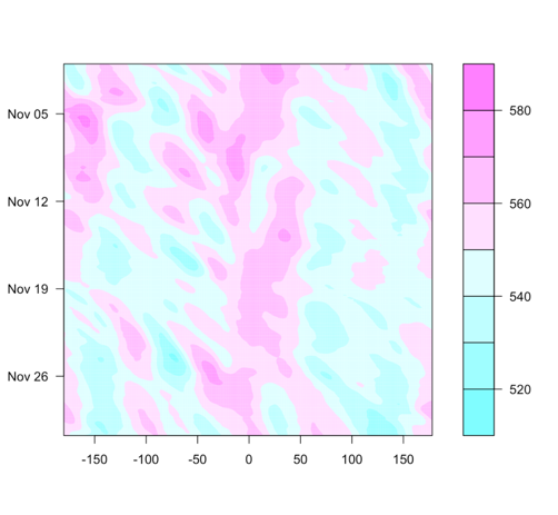
Let’s add in labels by running the code below:
Below is a larger version of the figure:
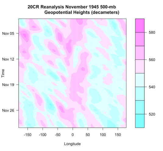
And there you have it! Your first Hovmöller diagram!
Interpret and Further Analyses
The last step is to interpret the diagram. High values are represented by the pinkish colors, while low values are the blueish colors. We see a downstream change from high values to low values, similar to the original. For reference, here is the original image next to the one we created.
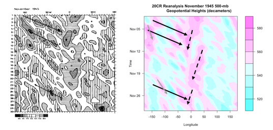
The solid black lines are again the group velocity, showing downstream development. The gray solid lines show the phase speed, moving slower than the group velocity. These two lines together (solid black and gray) represent the Rossby waves. There is another phenomenon going on, however. There are 3 westward moving ridges (high geopotential heights). These are highlighted by the black dashed lines and represent wider waves moving slowly west. In summary, this figure shows two phenomena going on, shorter waves (phase speed and group velocity) moving eastward and longer waves moving slowly west.
Depending on the question, further analyses may be needed. This could include performing an ARDL, spectrum or cross-spectrum analysis, or any of the other analyses we’ve learned in this course or in Meteo 815.