Motivation and Preamble
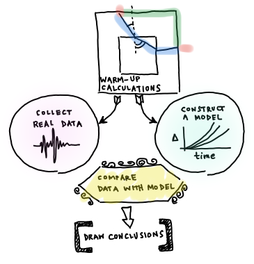
The Earth is optically opaque. Unlike the tank you used in the optics lab, you can't see through the Earth to verify what path a P wave takes on its way from an earthquake to a seismometer. How do we know what path a P wave takes? What data can we collect to help us find this out? We are going to take a two-step approach to answering these questions. We are going to collect some data from seismometers around the world that all recorded the same earthquake, and then we will use that data to plot a travel-time curve. We will then construct some models about what the data would look like given certain mantle properties. We will compare the data with our models to see if they match up or not.
What you will need:
You will need a plotting program, a scientific calculator, a protractor, and a straightedge to complete this problem set. Drawing software is only suggested if you have a program you are already adept at using, otherwise, sketch by hand.
Directions
You can save the P wave path worksheet to your computer, and use it to record your work. The worksheet is in Microsoft Word format. To work on this assignment, you can use a word processing program, or even do it all on paper as long as I can read the scanned pages. You will submit your worksheet electronically, so it must be in a format I can open. Ask me if you aren't sure whether your format is weird. The downloadable worksheet has the same problems as are written out below; the worksheet is just to save you copy-and-pasting effort. This website has a couple of screencasted hints that are not in the worksheet, though.
Part 1: Snell's Law Warm-Up Calculations
Before we start jumping right into the data and models, we will do some warm-up calculations involving how rays travel. The point of this is so we have some intuitive sense later on about the meaning of our data and models, and what we might expect them to look like. In this part of the problem set, you will make calculations involving the refraction of waves through media and you will trace ray paths through media. You will have to make some sketches. If you want to use drawing software, go ahead. If you want to make your sketches by hand and take pictures of them, that is also fine. When I grade your sketches I will not be using a protractor to judge the precision of your angles, but I will be looking to see if your angles are correct relative to each other on the same sketch. For example, if the angle of refraction should be greater than the angle of incidence in a particular problem then you need to draw it that way.
The Problems
1.1 Calculate the angle of refraction for a ray of light passing from air to water with an incident angle of 45°. Assume the index of refraction of water (nwater) is 1.33 and nair is 1. Sketch the path of the ray through the water layer. 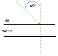
1.2 Calculate the angle of refraction for a ray of light passing from water to air with an incident angle of 30°. Assume the index of refraction of water (nwater) is 1.33 and nair is 1. Sketch the path of the ray through the air layer. 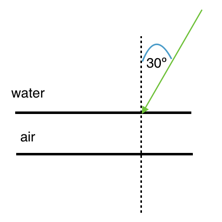
1.3 Suppose you have a ray of light that passes through three layers: air - water - air. The angle of incidence at the first air - water boundary is 20°. Calculate the angle of refraction at the first boundary in the diagram below and calculate both the angle of incidence and angle of refraction at the second (water - air) boundary. 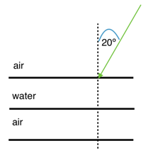
1.4 Now let's consider the path taken by a seismic wave instead of light. For the purposes of this calculation, we'll pretend the Earth is flat. An earthquake happens at the surface of a series of layers as pictured below. Consider a P wave that leaves the source along the path as shown in the cartoon and hits the boundary between the upper layer and the second layer with an angle of incidence of 30°. Given the transmitting velocities for a P wave in all the subsequent layers, sketch the path of the ray until it hits the bottom, and find all the angles of incidence and refraction along the way.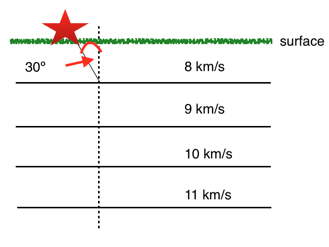
1.5 Let’s consider a seismic wave that passes through the square-shaped object below. In this object there is a fast center and an outer layer of slower material. The P wave leaves the source and hits the first boundary with an incident angle of 40°. Sketch the path taken by the P wave until it gets back to the outer surface of the square and calculate all the angles of incidence and refraction along the way.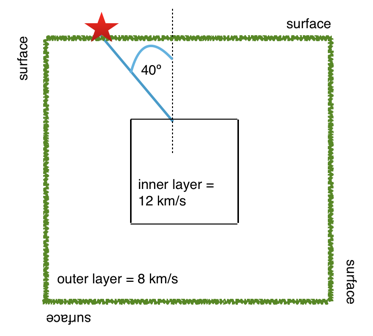
1.6 Now let’s say that same square-shaped object in #1.5 is actually homogeneous. Draw the path that the P wave would have followed to get from the source to the position of the “receiver” (where you calculated that it arrived at the outer surface in #1.5). Is the distance traveled as measured along the surface the same, shorter or longer as the distance as measured along the surface in #1.5? Is the actual path traversed by the P wave the same, shorter, or longer than the actual path traversed by the P wave in #1.5?
Road Check
Okay, so you just did a bunch of calculations and sketches. What's the upshot? Here's what we found out: Rays travel the fastest path they can. This will be a straight line path through a homogeneous solid, but might not be a straight line path in an object composed of different materials that transmit rays at different speeds. Rays change direction at the boundary between two materials.
Therefore, if the mantle is homogeneous then a P wave will take a straight line path with a constant velocity through it. If the mantle is not homogeneous then the P wave's velocity will not be constant all the way through and its path will not be a straight line. The obvious next step towards our goal of figuring out what path a P wave takes through the mantle is to collect some data about P wave velocities. We should look for data covering a variety of paths so we can compare if the velocities are all the same or not. What we want is to either go get data from a station that recorded P waves from earthquakes all over the world, or else get data from one earthquake that was recorded by stations all over the world.
We could do either one, but data is commonly archived by earthquake instead of by station, so it will be more convenient to collect data from a variety of stations that all recorded the same earthquake. Let's do it!
Part 2: Collecting data and making observations

In this part of the problem set, you will pick the arrival times of P waves on seismograms and use them to construct a travel time curve for P waves through the mantle. Then, you will compare this data to models of travel time curves for an assumed homogeneous mantle.
The seismograms for this activity are clickable thumbnails so you can work with a big version of each one. On this web page there are several hints about how to do most of the calculations.
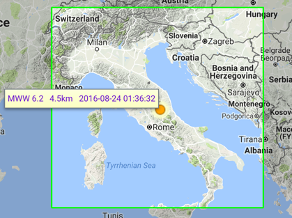
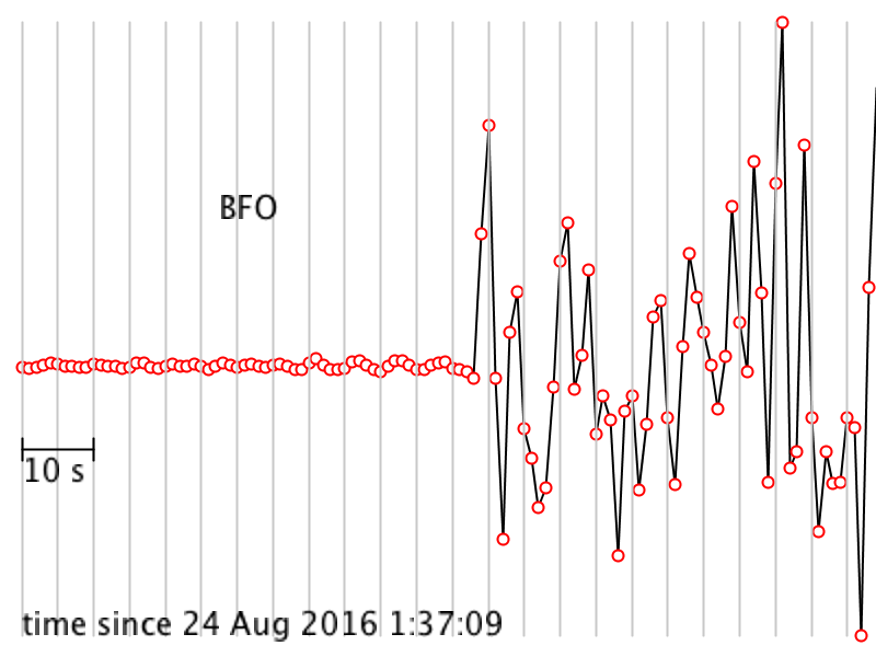
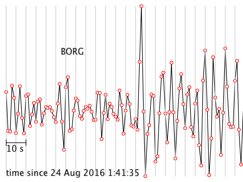
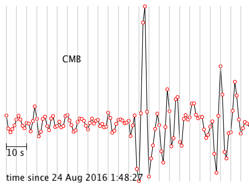
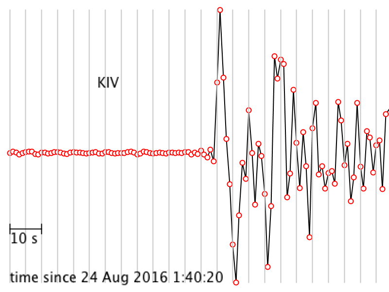
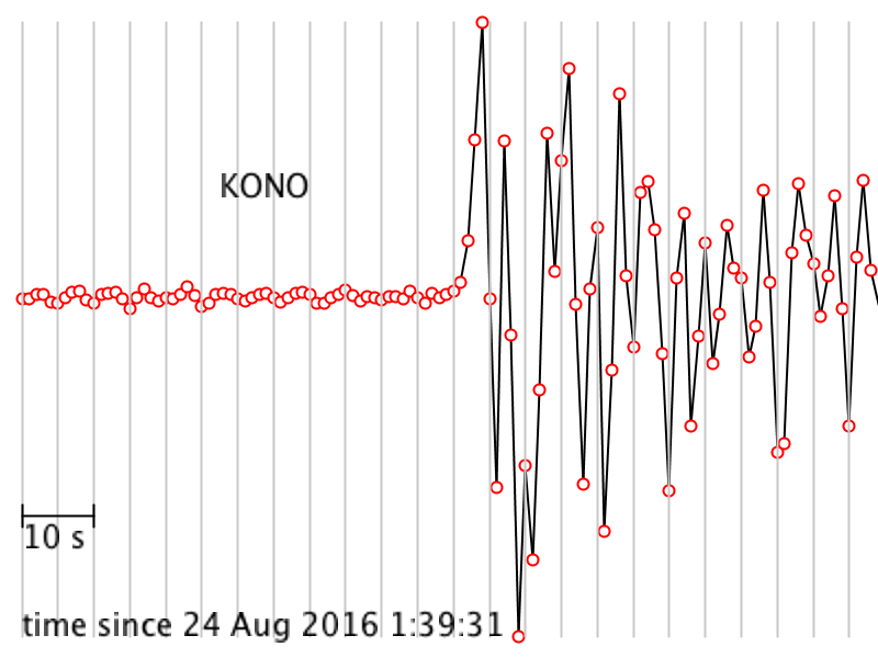
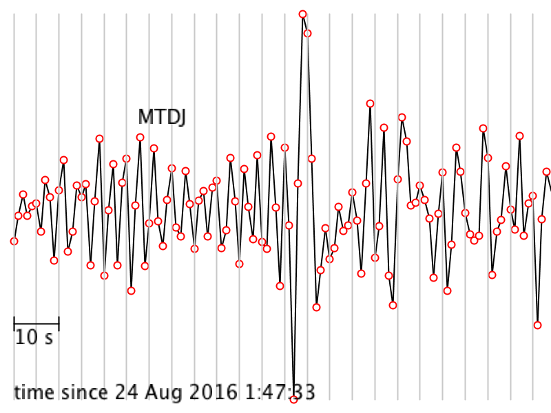
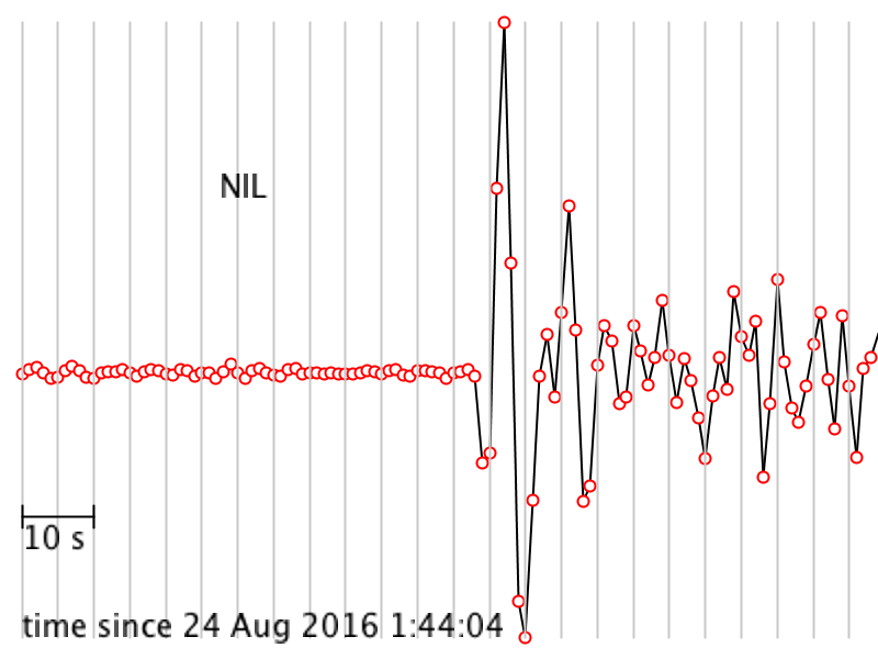
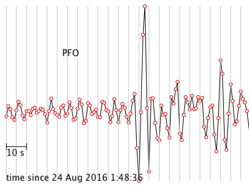
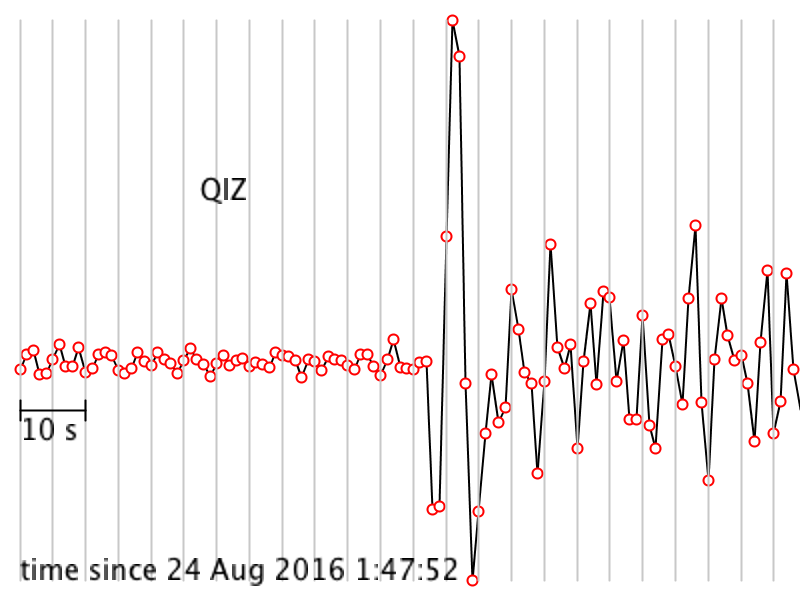
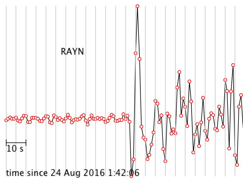
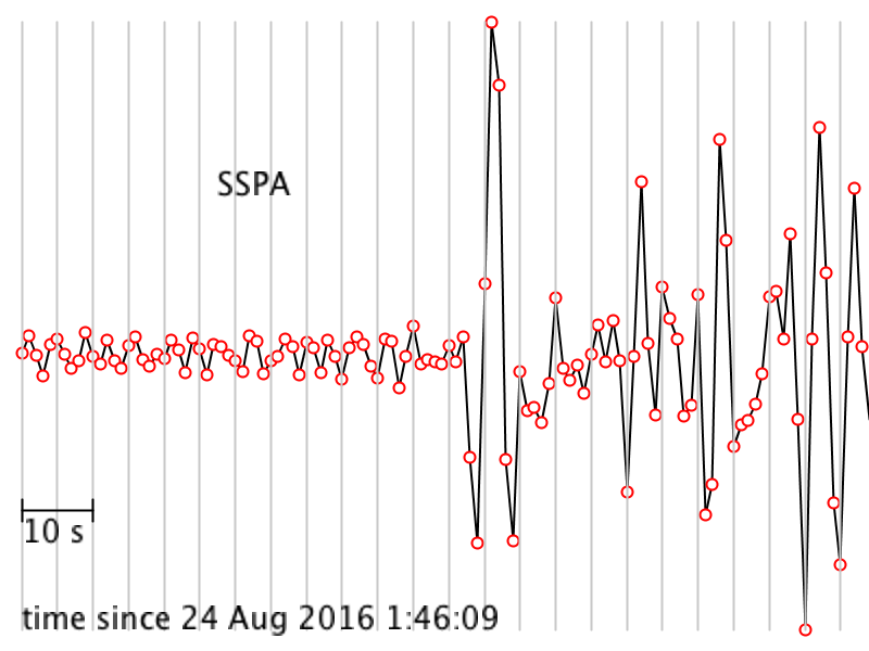
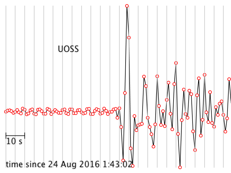
The seismograms you'll be working with are from the Amatrice, Italy, earthquake of 24 August 2016. Its location was 42.7226° N, 13.1871° E, and it happened at 01:36:32 UTC. All the seismogram times are also in UTC.
The Seismograms


The Problems
For #s 2.1, 2.2, and 2.3 I find it easiest to make a table in which I write down the station name in column 1, The P wave arrival time at that station in column 2, the travel time in column 3 and the distance in degrees in column 4. Doing so makes it easier to make plots and be organized. I am leaving it up to you to construct such a table, or if you hate tables, to ignore this advice.
2.1 For each seismogram, pick the arrival time of the P wave. The P wave is the first impulsive arrival that rises appreciably higher than the background noise level. It can take a bit of skill and practice to pick arrivals on a seismogram, but at least P waves are easier than the later arrivals.
My tutorial for picking the arrival time of a P wave (and a transcript)
2.2 Calculate the time it took the P wave to get to each station.
My tutorial for calculating P wave travel time (and a transcript)
2.3 Calculate the distance between each station and the event in degrees. In order to do this, you'll have to compute the great circle distance between the event and each station. Here is the formula for great circle distance between two points on the surface of a sphere: cos(d) = sin(a)sin(b) + cos(a)cos(b)cos|c| in which d is the distance in degrees, a and b are the latitudes of the two points and c is the difference between the longitudes of the two points. Jean-Paul Rodrigue, at Hofstra University, provides an excellent explanation and tutorial of how to calculate distance along a great circle path.
My tutorial for calculating great circle distance (and a transcript)
There is a nice website that will calculate the great circle distance for you and it will give you the answer in kilometers, so if you use it, divide your distances by 111.32 to get from kilometers to degrees in order to make your plot in #2.4.
2.4 Make a plot of distance in degrees vs. P wave travel time. Note that choice of which quantity to put on which axis depends on what you are trying to do with this data. Many seismologists put distance on the x axis and travel time on the y axis because then the slope of the data is the quantity known as the “slowness.” However, doing it the other way around is also quite common, especially if you are stacking record sections to make a plot. You can choose.
2.5 Which station was closest and which station was farthest away? What were the distances between the earthquake and each of these two stations? What was the difference in arrival time between those two stations?
2.6. This event was large enough that it was recorded by stations even farther away than the farthest station you worked with. Why didn't I make you pick P waves for stations that were farther away?
2.7 We know the travel time of the P wave to each station and we know the surface distance between the earthquake and each station but we don’t know the actual path the P wave took and we don’t know whether velocity was constant along that path or not (Remember that those are the two things we are trying to find out in this lab exercise). So when we calculate velocity, keep in mind that it is an apparent, average velocity. What is the apparent average velocity of the P wave for the closest station? What is the apparent average velocity of the P wave for the farthest station? Are they the same or not? If they are not the same, can the difference be attributed to rounding during calculations, mistakes in arithmetic, or other uncertainties?
2.8 Look at your plot from #2.4 and describe how the apparent average velocity changes with station distance, if it does. For example, are the data randomly scattered with no relationship among them? Is there a smooth variation with distance? If there’s a smooth variation, does velocity increase or decrease? Or, does the velocity stay about the same? Are there sudden jumps?
Road Check
Up until now we have been collecting and analyzing a dataset chosen to help us figure out if the Earth’s mantle is homogeneous or not. The next step is to predict what travel time data would look like if the mantle is in fact homogeneous. Then we can compare it to our actual data and see what we find out.
Part 3: Construct a model and compare it to the data
 We will construct a model plot of travel time vs distance (like the plot in #2.4) except that we will set the velocity to a constant and we will calculate what the travel time curves should look like instead of using real data. Doing this is not quite as trivial as you might guess. It takes a little bit of trigonometry to do this correctly.
The Problems
3.1 If the great circle distance between an earthquake and a station is 45º, what is the straight-line path distance through the Earth between them? (see hint cartoon and screencast below)
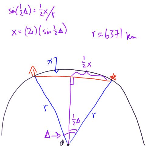
You can also read this transcript of me screencasting the right triangle sketch
Here is how to solve for the path length of a P wave through the mantle on the assumption that the mantle is homogeneous and transmits waves at the same speed regardless of depth.
I am just going to draw a hemisphere of the Earth. Here is the center of the Earth. Let us assume there is an earthquake that happens over here. And you have a seismometer over here that recorded a P wave. If the mantle is homogeneous it means that the P wave will travel a straight line path through the Earth from the earthquake to the seismometer. To solve this problem of what this distance x is, I am going to first draw a radius from the center of the Earth to my earthquake and another radius from the center of the Earth to the seismometer. This is an isosceles triangle because these two sides are both the radius of the Earth and then this other side here is the one we are trying to find. We also know something else about this triangle. We know this angle. This angle seismologists call delta, and it is exactly the great circle arc distance between the earthquake and the seismometer. You have already calculated delta for all the stations in this problem set. We drop a perpendicular line from x to the center of the Earth bisecting x and bisecting this angle delta. This is a right angle here, and this distance is one half x and this angle here is one half delta. The sine of one half delta is equal to the opposite side, which is one half x, divided by the hypotenuse, which is the radius of the Earth. Let us write that down. This is a fabulous expression because we know everything in it except x and we are trying to solve for x so that is awesome. Let us rearrange. x equals twice the radius times the sine of one half delta. If you want to find x you can just plug in delta, which you have already calculated, and the radius of the Earth, which we can take as 6371 km. That's a good approximation. And away you go. X is the distance between the earthquake and the station traversed by a P wave if you assume the mantle is homogeneous.
3.2 Suppose a P wave traveled along the path you calculated in #3.1 at a constant speed of 8 km/s. Calculate its travel time between the earthquake and the station.
3.3 Suppose a P wave traveled along the path you calculated in #3.1 at a constant speed of 10 km/s. Calculate its travel time between the earthquake and the station.
3.4 Suppose a P wave traveled along the path you calculated in #3.1 at a constant speed of 12 km/s. Calculate its travel time between the earthquake and the station.
3.5. Assume constant mantle velocities of 8, 10, and 12 km/sec. Draw the three travel-time curves that correspond to these velocities on one set of axes.
My tutorial for how to make your reference travel time curves now that you know how to calculate the straight-line P wave path and find the travel time for a single station. (and a transcript)
 3.6. Combine your plot from #2.4 and your plot from #3.5 on the same axes. Can your data be fit with a curve representing constant velocity? Feel free to try other values for the velocity if 8, 10, and 12 don’t work.
 3.7. Time to answer the big question from the beginning of the problem set! Does the P wave follow a straight line path through the mantle? How do you know? Lead me through your logic and your observations from this lab to answer this question.
Submitting your work
Please save your worksheet and name it like this:
L4_Ppath_AccessAccountID_LastName.doc (or whatever your file extension is).
For example, former Cardinals manager and hall of famer Whitey Herzog would name his file "L4_Ppath_dnh24_herzog.doc"--This naming convention is important, as it will help me make sure I match each submission up with the right student! You can look it up; his given name is Dorrel Norman Elvert Herzog. Upload your finished product to the Canvas assignment by the due date listed on the first page of the lesson.
Grading Criteria
I will use my general grading rubric for problem sets to grade this activity.