4.2 Attribute Measurement Scales

Chapter 2 focused upon measurement scales for spatial data, including map scale (expressed as a representative fraction), coordinate grids, and map projections (methods for transforming three dimensional to two dimensional measurement scales). You may know that the meter, the length standard established for the international metric system, was originally defined as one-ten-millionth of the distance from the equator to the North Pole. In virtually every country except the United States, the metric system has benefited science and commerce by replacing fractions with decimals, and by introducing an Earth-based standard of measurement.

Standardized scales are needed to measure non-spatial attributes as well as spatial features. Unlike positions and distances, however, attributes of locations on the Earth's surface are often not amenable to absolute measurement. In a 1946 article in Science, a psychologist named S. S. Stevens outlined a system of four levels of measurement meant to enable social scientists to systematically measure and analyze phenomena that cannot simply be counted. (In 1997, geographer Nicholas Chrisman pointed out that a total of nine levels of measurement are needed to account for the variety of geographic data.) The levels are important to specialists in geographic information because they provide guidance about the proper use of different statistical, analytical, and cartographic operations. In the following, we consider examples of Stevens' original four levels of measurement: nominal, ordinal, interval, and ratio.

4.2.1 Nominal Level

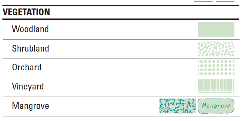
The term nominal simply means to relate to the word “name.” Simply put, nominal level data are data that are denoted with different names (e.g., forest, water, cultivated, wetlands), or categories. Data produced by assigning observations into unranked categories are nominal level measurements. In relation to terminology used in Chapter 1, nominal data are a type of categorical (qualitative) data. Specifically, nominal level data can be differentiated and grouped into categories by “kind,” but are not ranked from high to low. For example, one can classify the land cover at a certain location as woods, scrub, orchard, vineyard, or mangrove. There is no implication in this distinction, however, that a location classified as "woods" is twice as vegetated as another location classified "scrub."

Figure 4.3. Attribute data measured at the nominal level: Selected vegetation categories depicted on USGS topographic maps.

Credit: USGS.

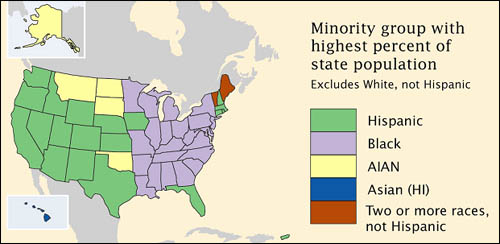
Although census data originate as individual counts, much of what is counted is individuals' membership in nominal categories. Race, ethnicity, marital status, mode of transportation to work (car, bus, subway, railroad...), and type of heating fuel (gas, fuel oil, coal, electricity...) are measured as numbers of observations assigned to unranked categories. For example, the map below, which appears in the Census Bureau's first atlas of the 2000 census, highlights the minority groups with the largest percentage of population in each U.S. state. Colors were chosen to differentiate the groups through a qualitative color scheme to show differences between the classes, but not to imply any quantitative ordering. Thus, although numerical data were used to determine which category each state is in, the map depicts the resulting nominal categories rather than the underlying numerical data.

Figure 4.4. Highest percent minority group by state.

Credit: Brewer & Suchan, 2001.

4.2.2 Ordinal Level

Like the nominal level of measurement, ordinal scaling assigns observations to discrete categories. Ordinal categories, however, are ranked, or ordered – as the name implies. It was stated in the preceding section that nominal categories such as "woods" and "mangrove" do not take precedence over one another, unless a set of priorities is imposed upon them. This act of prioritizing nominal categories transforms nominal level measurements to the ordinal level. Because the categories are not based upon a numerical value (just an indication of an order or importance), ordinal data are also considered to be categorical (or qualitative).

Figure 4.5. Attribute data measured at the ordinal level: Ranked categories of boundaries depicted on USGS topographic maps.

Credit: USGS.

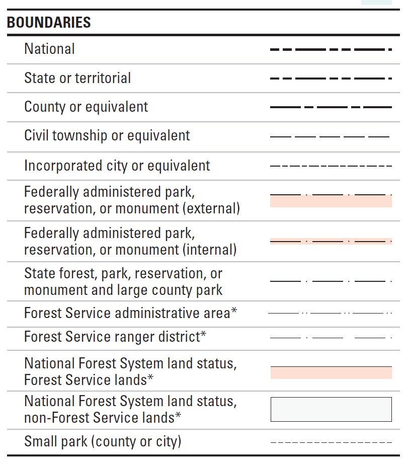
Examples of ordinal data often seen on reference maps include political boundaries that are classified hierarchically (national, state, county, etc.) and transportation routes (primary highway, secondary highway, light-duty road, unimproved road). Ordinal data measured by the Census Bureau include how well individuals speak English (very well, well, not well, not at all), and level of educational attainment (high school graduate, some college no degree, etc.). Social surveys of preferences and perceptions are also usually scaled ordinally.

Individual observations measured at the ordinal level are not numerical, thus should not be added, subtracted, multiplied, or divided. For example, suppose two 600-acre grid cells within your county are being evaluated as potential sites for a hazardous waste dump. Say the two areas are evaluated on three suitability criteria, each ranked on a 0 to 3 ordinal scale, such that 0 = completely unsuitable, 1 = marginally unsuitable, 2 = marginally suitable, and 3 = suitable. Now say Area A is ranked 0, 3, and 3 on the three criteria, while Area B is ranked 2, 2, and 2. If the Siting Commission was to simply add the three criteria, the two areas would seem equally suitable (0 + 3 + 3 = 6 = 2 + 2 + 2), even though a ranking of 0 on one criteria ought to disqualify Area A.

4.2.3 Interval Level

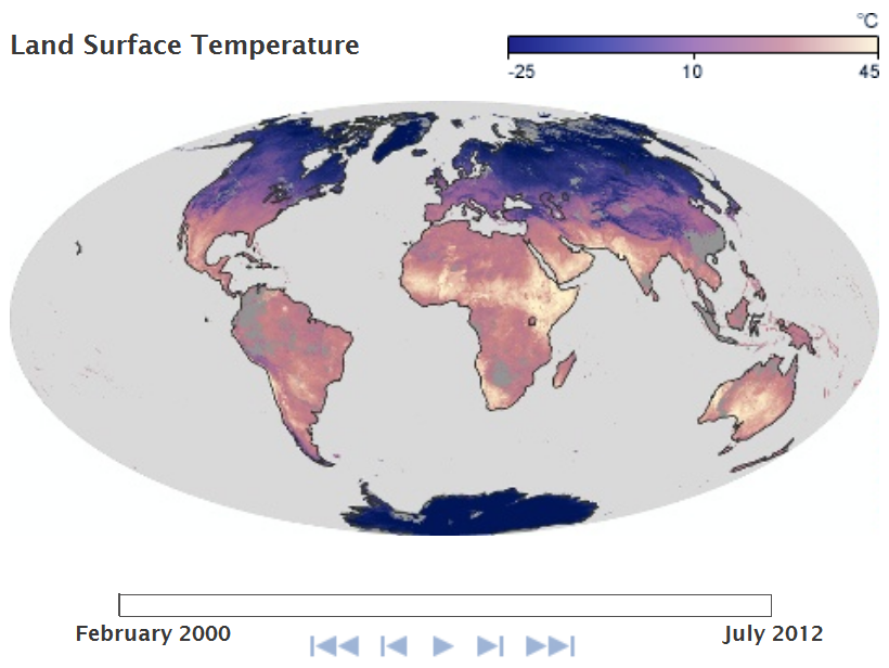
Unlike nominal- and ordinal-level data, which are categorical (qualitative) in nature, interval level data are numerical (quantitative). Examples of interval level data include temperature and year. With interval level data, the zero point is arbitrary on the measurement scale. For instance, zero degrees Fahrenheit and zero degrees Celsius are different temperatures.

Figure 4.6. Global Land Surface Temperature Map. This map is a screen capture from an interactive animated map provided by NASA. If you follow the link to the site, you can plan an animation of global temperature that runs from February 2000 until July 2012.

Credit: NASA Earth Observatory.

4.2.4 Ratio Level

Similar to interval level data, ratio level data are also numerical (quantitative). Examples of ratio level data include distance and area (e.g., acreage). Unlike the interval level measurement scale, the zero is not arbitrary for ratio level data. For example, zero meters and zero feet mean exactly the same thing, unlike zero degrees Fahrenheit and zero degrees Celsius (both temperatures). Ratio level data also differs from interval level data in the mathematical operations that can be performed with the data. An implication of this difference is that a quantity of 20 measured at the ratio scale is twice the value of 10 (20 meters is twice the distance of 10 meters), a relation that does not hold true for quantities measured at the interval level (20 degrees is not twice as warm as 10 degrees).

4.2.5 Interval and Ratio Level Data

The scales for both interval and ratio level data are similar in so far as units of measurement are arbitrary (Celsius versus Fahrenheit and English versus metric units). These units of measurement are split evenly for each successive value (e.g., 1 meter, 2 meters (add 1 meter), 3 meters (add 1 meter), 4 meters (add 1 meter). Because interval and ratio level data represent positions along continuous number lines, rather than members of discrete categories, they are also amenable to analysis using statistical techniques.

Try This: Surf the Internet and find an interesting map, visualizing data from two of the different attribute measurement scales: nominal, ordinal, interval, and ratio. Provide a written citation for the source of each map as well as one sentence describing how each map uses nominal, ordinal, interval or ratio level data.

4.2.6 Attribute Measurement Level Operations

One reason that it's important to recognize levels of measurement is that different analytical operations are possible with data at different levels of measurement (Chrisman 2002). Some of the most common operations include:

• Group: Categories of nominal and ordinal data can be grouped into fewer categories. For instance, grouping can be used to reduce the number of land use/land cover classes from, for instance, four (residential, commercial, industrial, parks) to one (urban).

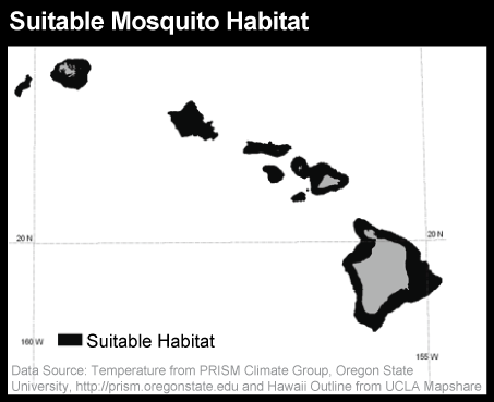
• Isolate: One or more categories of nominal, ordinal, interval, or ratio data can be selected, and others set aside. For example, consider a range of temperature readings taken over a large area. Only a subset of those temperatures are suitable for mosquito survival, and health officials can select and isolate areas based upon a specific temperature range that is likely there to take action in order to reduce the threat of a West Nile Virus or Dengue Fever outbreak from these mosquitoes.

Figure 4.7. Potential Mosquito Habitat Map based on temperature.

Credit: Jennifer M. Smith, Department of Geography, The Pennsylvania State University.

• Difference: The difference of two interval-level observations (such as two calendar years) can result in one ratio level observation (such as one age). For example, in 2012 (a year is an interval level value), someone born in 2000 (also interval level, of course) is 12 years old (age is ratio level since it has a definite zero).
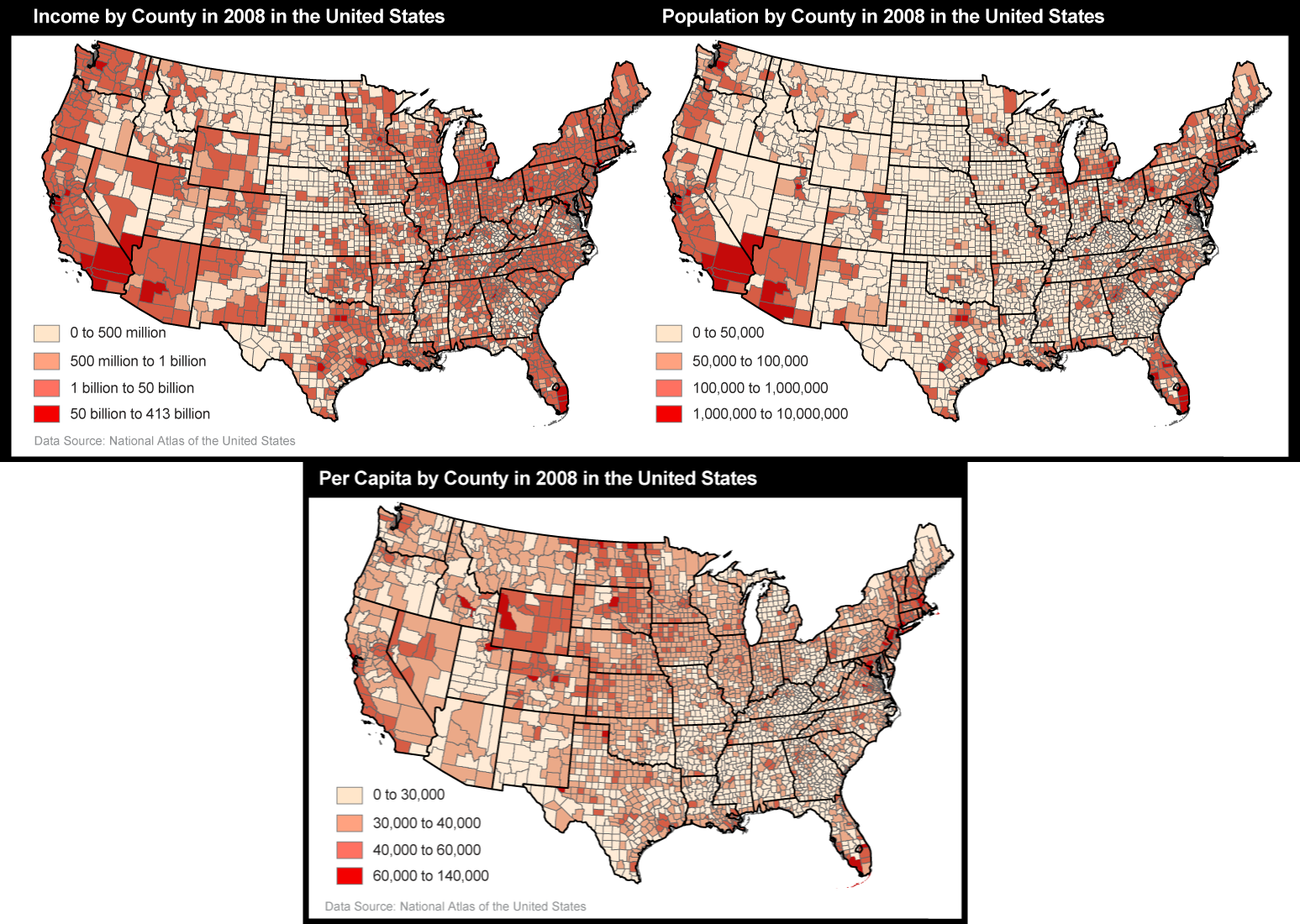
• Other arithmetic operations: Two or more compatible sets of interval or ratio level data can be added or subtracted. Only ratio level data can be multiplied or divided. For example, the per capita (average) income of an area can be calculated by dividing the sum of the income (ratio level) of every individual in that area (ratio level), by the number of persons (ratio level) residing in that area (a second ratio level variable).

Figure 4.8. Total Income, Population, Per Capita

Credit: Jennifer M. Smith, Department of Geography, The Pennsylvania State University.

• Classification: Numerical data (at interval and ratio level) can be sorted into classes, typically defined as non-overlapping numerical data ranges as discussed in Chapter 3.2.6. These classes are frequently treated as ordinal level categories for thematic mapping with the symbolization on choropleth maps, for example, emphasizing rank order without attempting to represent the actual magnitudes.