3.10.2 Accessing features and geoprocessing tools

The ArcGIS Python API also provides the functionality to access individual features in a feature layer, to manipulate layers, and to run analyses from a large collection of GIS tools including typical GIS geoprocessing tools. Most of this functionality is available in the different submodules of arcgis.features. To give you a few examples, let’s continue with the city feature service we still have in variable neCitiesFS from the previous section. A feature service can actually have several layers but, in this case, it only contains one layer with the point features for the cities. The following code example accesses this layer (neCitiesFE.layers[0]) and prints out the names of the attribute fields of the layer by looping through the ...properties.fields list of the layer:

for f in neCitiesFS.layers[0].properties.fields:
	print(f)

When you try this out, you should get a list of dictionaries, each describing a field of the layer in detail including name, type, and other information. For instance, this is the description of the STATEABB field:

{
 "name": "STATEABB",
 "type": "esriFieldTypeString",
 "actualType": "nvarchar",
 "alias": "STATEABB",
 "sqlType": "sqlTypeNVarchar",
 "length": 10,
 "nullable": true,
 "editable": true,
 "domain": null,
 "defaultValue": null
 }

The query(...) method allows us to create a subset of the features in a layer using an SQL query string similar to what we use for selection by attribute in ArcGIS itself or with arcpy. The result is a feature set in ESRI terms. If you look at the output of the following command, you will see that this class stores a JSON representation of the features in the result set. Let’s use query(...) to create a feature set of all the cities that are located in Pennsylvania using the query string "STATEABB"='US-PA' for the where parameter of query(...):

paCities = neCitiesFS.layers[0].query(where='"STATEABB"=\'US-PA\'')
print(paCities.features)
paCities

Output: 
[{"geometry": {"x": -8425181.625237303, "y": 5075313.651659228}, 
"attributes": {"FID": 50, "OBJECTID": "149", "UIDENT": 87507, "POPCLASS": 2, "NAME": 
"Scranton", "CAPITAL": -1, "STATEABB": "US-PA", "COUNTRY": "USA"}}, {"geometry": 
{"x": -8912583.489066456, "y": 5176670.443556941}, "attributes": {"FID": 53, 
"OBJECTID": "156", "UIDENT": 88707, "POPCLASS": 3, "NAME": "Erie", "CAPITAL": -1, 
"STATEABB": "US-PA", "COUNTRY": "USA"}}, ...  ]
<FeatureSet> 10 features

Of course, the queries we can use with the query(...) function can be much more complex and logically connect different conditions. The attributes of the features in our result set are stored in a dictionary called attributes for each of the features. The following loop goes through the features in our result set and prints out their name (f.attributes['NAME']) and state (f.attributes['STATEABB']) to verify that we only have cities for Pennsylvania now:

for f in paCities:
	print(f.attributes['NAME'] + " - "+ f.attributes['STATEABB'])

Output: 
Scranton - US-PA
Erie - US-PA
Wilkes-Barre - US-PA
...
Pittsburgh - US-PA

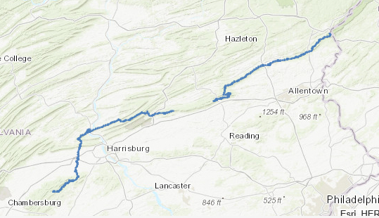
Now, to briefly illustrate some of the geoprocessing functions in the ArcGIS Python API, let’s look at the example of how one would determine the parts of the Appalachian Trail that are within 30 miles of a larger Pennsylvanian city. For this we first need to upload and publish another data set, namely one that’s representing the Appalachian Trail. We use a data set that we acquired from PASDA for this, and you can download the DCNR_apptrail file here. As with the cities layer earlier, there is a very small chance that this will not display for you - but you should be able to continue to perform the buffer and intersection operations. The following code uploads the file to AGOL (don’t forget to adapt the path and add your initials or ID to the name!), publishes it, and adds the resulting trail feature service to your cityMap from above:

appTrail = gis.content.add({'type': 'Shapefile'}, r'C:\489\L3\dcnr_apptrail_2003.zip')
appTrailFS = appTrail.publish()
cityMap.add_layer(appTrailFS, {})

Figure 3.23 Map widget now showing the cities and trail layers

Next, we create a 30 miles buffer around the cities in variable paCities that we can then intersect with the Appalachian Trail layer. The create_buffers(...) function that we will use for this is defined in the arcgis.features.use_proximity module together with other proximity based analysis functions. We provide the feature set we want to buffer as the first parameter, but, since the function cannot be applied to a feature set directly, we have to invoke the to_dict() method of the feature set first. The second parameter is a list of buffer distances allowing for creating multiple buffers at different distances. We only use one distance value, namely 30, here and also specify that the unit is supposed to be ‘Miles’. Finally, we add the resulting buffer feature set to the cityMap above.

from arcgis.features.use_proximity import create_buffers
bufferedCities = create_buffers(paCities.to_dict(), [30], units='Miles')
cityMap.add_layer(bufferedCities, {})

Figure 3.24 Map widget with buffers created by the previous code example

As the last step, we use the overlay_layers(...) function defined in the arcgis.features.manage_data module to create a new feature set by intersecting the buffers with the Appalachian Trail polylines. For this we have to provide the two input sets as parameters and specify that the overlay operation should be ‘Intersect’.

from arcgis.features.manage_data import overlay_layers
trailPartsCloseToCity = overlay_layers(appTrailFS, bufferedCities, overlay_type='Intersect')

We show the result by creating a new map ...

resultMap = gis.map('Pennsylvania')
resultMap

... and just add the features from the resulting trailPartsCloseToCity feature set to this map:

resultMap.add_layer(trailPartsCloseToCity)

The result is shown in the figure below.

Figure 3.25 New map widget showing the final result of our analysis