QGIS has a toolbox system and visual workflow building component somewhat similar to ArcGIS and its Model Builder. It is called the QGIS processing framework and comes in the form of a plugin called Processing that is installed by default. You can access it via the Processing menu in the main menu bar. All algorithms from the processing framework are available in Python via a QGIS module called processing. They can be combined to solve larger analysis tasks in Python and can also be used in combination with the other qgis methods discussed in the previous sections.
We can get a list of all processing algorithms currently registered with QGIS with the command QgsApplication.processingRegistry().algorithms(). Each processing object in the returned list has an identifying name that you can get via its id() method. The following command, which you can try out in the QGIS Python console, uses this approach to print the names of all algorithms that contain the word “clip”:
[x.id() for x in QgsApplication.processingRegistry().algorithms() if "clip" in x.id()]
Output:

['gdal:cliprasterbyextent', 'gdal:cliprasterbymasklayer','gdal:clipvectorbyextent', 'gdal:clipvectorbypolygon', 'native:clip', 'saga:clippointswithpolygons', 'saga:cliprasterwithpolygon', 'saga:polygonclipping']
As you can see, there are processing versions of algorithms coming from different sources, e.g. natively built into QGIS vs. algorithms based on GDAL. The function algorithmHelp(…) allows you to get some documentation on an algorithm and its parameters. Try it out with the following command:
processing.algorithmHelp("native:clip")
To run a processing algorithm, you have to use the run(…) function and provide two parameters: the id of the algorithm and a dictionary that contains the parameters for the algorithm as key-value pairs. run(…) returns a dictionary with all output parameters of the algorithm. The following example illustrates how processing algorithms can be used to solve the task of clipping a points of interest shapefile to the area of El Salvador, reusing the two data sets from homework assignment 2 (Section 2.10). This example is intended to be run as a standalone program again and most of the code is required to set up the QGIS environment needed, including initializing the Processing environment.
The start of the script looks like in the example from the previous section:
import os,sys
import qgis
import qgis.core

qgis_prefix = os.getenv("QGIS_PREFIX_PATH")
qgis.core.QgsApplication.setPrefixPath(qgis_prefix, True)
qgs = qgis.core.QgsApplication([], False)
qgs.initQgis()
After, creating the QGIS environment, we can now initialize the processing framework. To be able to import the processing module we have to make sure that the plugins folder is part of the system path; we do this directly from our code. After importing processing, we have to initialize the Processing environment and we also add the native QGIS algorithms to the processing algorithm registry.
# Be sure to change the path to point to where your plugins folder is located
# it may not be the same as this one.
sys.path.append(r"C:\OSGeo4W\apps\qgis-ltr\python\plugins")
import processing
from processing.core.Processing import Processing
Processing.initialize()
qgis.core.QgsApplication.processingRegistry().addProvider(qgis.analysis.QgsNativeAlgorithms())
Next, we create input variables for all files involved, including the output files we will produce, one with the selected country and one with only the POIs in that country. We also set up input variables for the name of the country and the field that contains the country names.
poiFile = r'C:\489\L2\assignment\OSMpoints.shp'
countryFile = r'C:\489\L2\assignment\countries.shp'
pointOutputFile = r'C:\489\L2\assignment\pointsInCountry.shp'
countryOutputFile = r'C:\489\L2\assignment\singleCountry.shp'

nameField = "NAME"
countryName = "El Salvador"
Now comes the part in which we actually run algorithms from the processing framework. First, we use the qgis:extractbyattribute algorithm to create a new shapefile with only those features from the country data set that satisfy a particular attribute query. In the dictionary with the input parameters for the algorithm, we specify the name of the input file (“INPUT”), the name of the query field (“FIELD”), the comparison operator for the query (0 here stands for “equal”), and the value to which we are comparing (“VALUE”). Since the output will be written to a new shapefile, we don’t really need the output dictionary that we get back from calling run(…) but the print statement shows how this dictionary in this case contains the name of the output file under the key “OUTPUT”.
output = processing.run("qgis:extractbyattribute", { "INPUT": countryFile, "FIELD": nameField, "OPERATOR": 0, "VALUE": countryName, "OUTPUT": countryOutputFile  })
print(output['OUTPUT'])
To perform the clip operation with the new shapefile from the previous step, we use the “native:clip” algorithm. The input paramters are the input file (“INPUT”), the clip file (“OVERLAY”), and the output file (“OUTPUT”). Again, we are just printing out the content stored under the “OUTPUT” key in the returned dictionary. Finally, we exit the QGIS environment.
output = processing.run("native:clip", { "INPUT": poiFile, "OVERLAY": countryOutputFile, "OUTPUT": pointOutputFile })
print(output['OUTPUT'])

qgs.exitQgis()
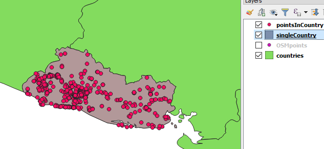
Below is how the resulting two layers should look when shown in QGIS in combination with the original country layer.
In this section, we showed you how to perform common GIS operations with the QGIS Python API. Once again we have to say that we are only scratching the surface here; the API is much more complex and powerful, and there is hardly anything you cannot do with it. What we have shown you will be sufficient to understand the code from the two walkthroughs of this lesson, but, if you want more, below are some links to further examples. Keep in mind though that since QGIS 3 is not that old yet, some of the examples on the web have been written for QGIS 2.x. While many things still work in the same way in QGIS 3, you may run into situations in which an example won’t work and needs to be adapted to be compatible with QGIS 3.