8.5 Gradients: How to Find Them
The gradient of a variable quantifies the magnitude and direction of the maximum change of the variable as a function of distance in space. For instance, the temperature gradient gives the maximum amount of temperature change in space and the direction of that maximum temperature change. Thus, a gradient is a vector.
We can find the gradient in Cartesian coordinates by using the del operator, which is also called the nabla or gradient operator, which is a vector that finds the partial derivative of a variable (please review 8.1) in each direction.
To see how we can calculate gradients, lets start with the commonly used gradient: the horizontal temperature gradient. Look at the surface temperature map for the United States on 8 September 2012.
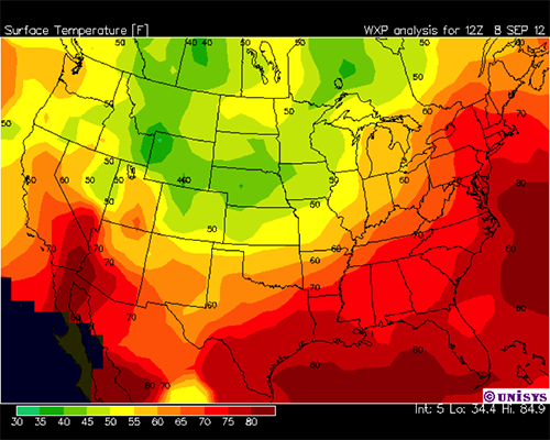
With the temperature data that was used to generate the map above, a computer can easily calculate the gradients for every location. However, you can get a better understanding of gradients by using a map, ruler, and the following mathemantical equations to estimate gradients. First, we show you how to find distances on a map using a ruler. Watch this video (2:12) on finding distances:
We're often interested in finding distances on a map so that we can calculate quantities we are interested in, such as the temperature gradient. Note first that often the projection of the map that we have does not have east-west, parallel, and straight across. In fact, the east-west line is curved a little bit, so take that into account when you're doing your calculations. Also note the north-south lines run a little bit not parallel as well. So how do we find distances? Well, there are many different ways, but one good way is to take a known distance on the map, scale it with a ruler, and then use that ruler in other places to give us distances in other places. So for instance, we know that the height of Pennsylvania between the two parallel borders, the north and south borders is 135 nautical miles. So we can scale that with a ruler, and I have a ruler here. I put the ruler in, and I see, in this particular case, the distance between the two is just about exactly 1 centimeter or 10 millimeters. So what that means is each millimeter on my scale is equal to 13.5 nautical miles on the map. So then I can use this in other places to measure other distances. So for instance, if I want to know the height of Kansas between its parallel North and South borders, I can put my ruler on there. And if I look carefully, I get a number that's about 13 and 1/2 millimeters. So 13 and 1/2 times 13 and 1/2 is about 182. And that's what I would say this distance is. The actual distance is 180 nautical miles, so in fact, the scaling I have is actually pretty good.
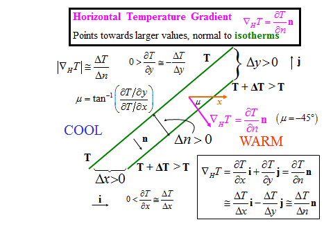
We can calculate a gradient for every point on the map, but to do this we need to know the change in the temperature over a distance that is centered on our chosen point. One approach is to calculate the gradients in the x and y directions independently and then determine the magnitude by:
and the direction by:
The partial derivatives are approximately equal to changes over small distances. Let's assume that the temperature gradient is approximately constant around a location. Then, integrating the equation 8.11, which is the definition of a horizontal gradient, yields
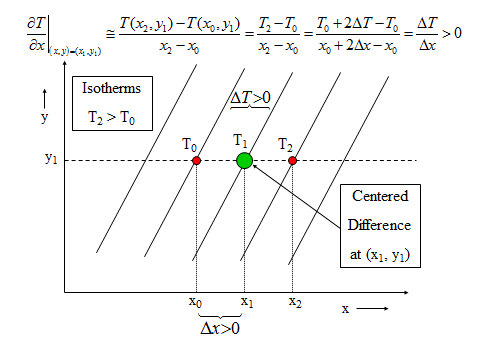
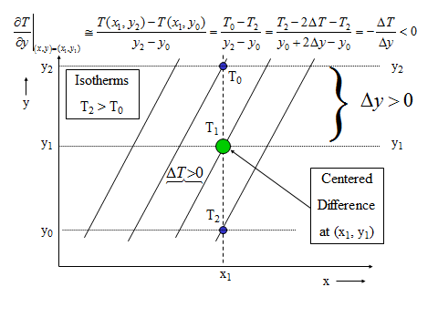
We can program a computer to do these calculations. However, often we just want to estimate the gradient. The gradient can be determined by looking at the contours on either side of the point and computing the change in temperature over the distance. These partial derivatives can be approximated by small finite changes in temperatures and distances, so that is replaced by in all places in these equations. We can calculate gradients by using “centered differences” as shown in the figures below.
We then calculate the magnitude with Equation [8.12] and the direction with Equation [8.13], where we replace the partial derivatives with the small finite differences in all places in these equations.
The magnitude and direction are:
When you calculate the arctangent, keep in mind that the tangent function has the same values every 180o or every π radians. If you get an answer for the arctangent that is 45o, how do you know whether the angle is really 45o or 45o + 180o = 225o? The gradient vector always points towards higher values, so always choose the angle so that the gradient vector points toward the warmer air. Alternatively, if ∂T/∂x is greater than 0, choose the value of the arctangent between –90o and 90o, whereas if ∂T/∂x is less than 0, add 180o.
Recap of the process for calculating the temperature gradient:
- Determine the distance scale by any means that you can. Sometimes it is given to you; sometimes you can scale off a ruler; sometimes you just estimate it using the size of known boundaries.
- Determine the spacing between the isotherms.
- Find the temperature change in the x and y directions using the centered difference method. These two numbers, , are needed to calculate both the gradient magnitude and the gradient direction. Note that can be either positive or negative.
- Calculate the magnitude by finding the square root of the squares of the gradients in the x and y directions (i.e., ).
- Calculate the direction of the gradient vector by finding the arctangent of the y-gradient divided by the x-gradient. Pay attention to the direction—make sure that it points toward the warmer air.
Now watch this video (3:52) on finding gradients:
We can calculate the gradient by using the method that's described in the lesson. Let's pick a point in Pennsylvania about here, and then we'll calculate the gradient for that point. We will first look at the gradient in the x direction which goes along, and it's parallel with the North and South boundaries of Pennsylvania. We'll use the method of center differences that's described. We'll look at this contour here, this isotherm, and this one over here on the other side. And we note that this distance here is very, very similar to the distance of Pennsylvania between the parallel borders, which is 135 nautical miles. And so each one of these contours is four degrees Fahrenheit. So we have two of them, so 8 divided by 135 nautical miles gives us a gradient in the x direction of 0.059 degrees Fahrenheit per nautical miles. Now we can do the y direction, so we pick two points here. One here and one about here to be on the gradients. And we note that this is a little bit more than half the height of Pennsylvania. It's actually about 80 nautical miles. But also note that as y goes more positive, the temperature becomes more negative and therefore, we have to use minus 8 over 80. And we get, for the gradient in the y direction, minus 0.1 degrees Fahrenheit per nautical miles. When we put these in to get the magnitude-- it's the square root of the squares-- we see that we end up with 0.12 degrees Fahrenheit per nautical mile with a magnitude of the gradient. To find the direction of the gradient we see that mu, the angle with respect to the x-axis-- so this is a math angle. It's equal to the arctangent of the gradient in y divided by the gradient in x. And so that would be the arctangent of minus 0.1 over 0.059, which is minus 59 degrees. And that is, of course, measured from the x-axis here. So that is measured from this direction here like this, and so that's minus 59. And it's the same as if we went all the way around and we would get 301 for alpha if we were looking at the math angle. Now, we can look and get an idea about gradients and other places really quickly, so let's just take this point in Central Oregon. So now x is going like this over here, and so we see that the gradient in the East West direction, or x direction is-- to go to another country you have to go very, very far, and so that would be 8 degrees. It's so far the really the gradient is essentially 0. Whereas if we go in the North South direction-- that is in the y direction here-- we see that there's quite a substantial distance here. And so, since this is 8 degrees, just like this is 8 degrees over here, then what that means is the gradient is going to be quite a bit smaller in this direction than it is in Pennsylvania here where the isotherms are much, much closer together. So we would expect a gradient that's a fourth or a fifth of the gradient that we got for Pennsylvania, and so it'll be very weak. Nonetheless, it'll point toward the hotter air, and it'll look something like this.
A word about finding gradients in the real world. Sometimes the centered differences method is difficult to apply because the gradient is too much east–west or north–south. For instance, in the temperature map at the beginning of this section, the x-gradient is hard to determine by the centered difference method in the Oklahoma panhandle and the y-gradient is hard to determine in central Pennsylvania because in both cases, the temperature hardly changes in those directions. In these cases, you could say that the gradient in that direction equals 0, but then your computer program might have a hard time finding the arctangent. One way around this problem is to put in a very small number for the gradient in that direction, say 1 millionth of your typical gradient numbers, to do the calculation.
A second word about finding gradients in the real world. When you are finding temperature gradients from a temperature map, it is sometimes hard to determine the temperature gradient at some locations because the isotherms are not evenly spaced and can be curvy. Don't despair! Use your best judgment as to what the gradients are. Check your answers for the magnitude and direction of the temperature gradient vector by estimating the magnitude and direction by eyeballing the normal to the isotherms at that location and pointing the gradient vector to the warmer air. If your calculated direction is very different from your eyeballed value by more than, say, 45o, check your math.
Quiz 8-3: Grading your gradients.
- Find Practice Quiz 8-3. You may complete this practice quiz as many times as you want. It is not graded, but it allows you to check your level of preparedness before taking the graded quiz.
- When you feel you are ready, take Quiz 8-3. You will be allowed to take this quiz only once. Good luck!