
We will start out our discussion of climate models with the simplest possible conceptual models for modeling Earth's climate. These models include different variants on the so-called Energy Balance Model. An Energy Balance Model or 'EBM' does not attempt to resolve the dynamics of the climate system, i.e., large-scale wind and atmospheric circulation systems, ocean currents, convective motions in the atmosphere and ocean, or any number of other basic features of the climate system. Instead, it simply focuses on the energetics and thermodynamics of the climate system.
We will start our discussion of EBMs with the so-called Zero Dimensional EBM—the simplest model that can be invoked to explain, for example, the average surface temperature of the Earth. In this very simple model, the Earth is treated as a mathematical point in space—that is to say, there is no explicit accounting for latitude, longitude, or altitude, hence we refer to such a model as 'zero dimensional'. In the zero-dimensional EBM, we solve only for the balance between incoming and outgoing sources of energy and radiation at the surface. We will then build up a little bit more complexity, taking into account the effect of the Earth's atmosphere—in particular, the impact of the atmospheric greenhouse effect—through use of the so-called "gray body" variant of the EBM.
Zero Dimensional EBM
The zero dimensional ('0d') EBM simply models the balance between incoming and outgoing radiation at the Earth's surface. As you'll recall from your review of radiation balance in the previous section, this balance is in reality quite complicated, and we have to make a number of simplifying assumptions if we are to obtain a simple conceptual model that encapsulates the key features.
For those who are looking for more technical background material, see this "Zero-dimensional Energy Balance Model" online primer (NYU Math Department). We will treat the topic at a slightly less technical level than this, but we still have to do a bit of math and physics to be able to understand the underlying assumptions and appreciate this very important tool that is used in climate studies.
We will assume that the amount of shortwave radiation absorbed by the Earth is simply , where S is the Solar Constant (roughly 1370 W /m2 but potentially variable over time) and α is the average reflectivity of Earth's surface looking down from space, i.e., the 'planetary albedo', accounting for reflection by clouds and the atmosphere as well as reflective surface of Earth including ice (value of roughly 0.32 but also somewhat variable over time).
We will assume that the outgoing long wave radiation is given simply by treating the Earth as a 'black body' (this is a body that absorbs all radiation incident upon it). The Stefan-Boltzman law for black body radiation holds that an object emits radiation in proportion to the 4th power of its temperature, i.e., the flux of heat from the surface is given by
where σ is known as the Stefan-Boltzmann constant, and has the value ; ε is the emissivity of the object (unitless fraction) — a measure of how 'good' a black body the object is over the range of wavelengths in which it is emitting radiation; and Ts (K) is the surface temperature. For the relatively cold Earth, the radiation is primarily emitted in the infrared regime of the electromagnetic spectrum, and the emissivity is very close to one.
We will approximate the surface temperature, TS, as representing the average 'skin temperature' of an Earth covered with 70% ocean (furthermore, we will treat the ocean as a mixed layer of average 70m depth—this ignores the impacts of heat exchange with the deep ocean, but is not a bad first approximation). We can then approximate the thermodynamic effect of the mixed layer ocean in terms of an effective heat capacity of the Earth's (land+ocean) surface, . The condition of energy balance can then be described in terms of the thermodynamics, which states that any change in the internal energy per unit area per unit time (<) must balance the rate of net heating, which is the difference between the incoming shortwave and outgoing longwave radiation. Mathematically, that gives:
Let's suppose that the incoming radiation (the first term on the right hand side) were larger than the outgoing radiation (the second term on the right hand side). Then the entire right-hand side would be positive, which means that the left-hand side, the rate of change of Ts over time, must also be positive. In other words, Ts must be increasing. This, in turn, means that the outgoing radiation must increase, which will eventually bring the two terms on the right hand side into balance. At this point, there is no longer any change of Ts with time, i.e., we achieve an equilibrium.
In equilibrium, the time derivative term is, by definition, zero, and we thus must have equality between the outgoing and incoming radiation, i.e., between the two terms on the right-hand side of equation 1. This yields the purely algebraic expression
The factor of 1/4 comes from the fact (see Figure 4.1, below) that the Earth is emitting radiation over the entirety of its surface area (4πR2 where R is the radius of the earth), but at any given time only receiving incoming (solar) radiation over its cross-sectional area, πR2.
It turns out that since the Earth's surface temperature varies over a relatively small range (less than 30° K) about its mean long-term temperature (in the range of O° C, or 273° K), i.e., it varies only by at most 10% or so, it is valid to approximate the 4th degree term in equation (1) by a linear relationship, i.e.,
A and B, thus defined, have the approximate values: ;
Such an approximation is often used in atmospheric science and other areas of physics when appropriate, and is called linearization.
Using this approximation, we can readily solve for TS as
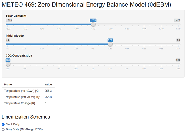
You might find it rather disappointing that, after all the work we did above to develop a realistic Energy Balance Model for Earth's climate, we were way off. Our EBM indicates that, given appropriate parameter values (i.e., ), the Earth should be a frozen planet with TS = 255° K, rather than the far more hospitable TS= 288° K we actually observe. Our model gave a result that was a whopping 33° C (roughly 60° F) too cold!
Think About It!
What do you think we forgot?
Click for answer.
So, how do we include the effect of the atmospheric greenhouse effect in a simple way? That is the topic of our next section.