Prioritize...
In this section, we'll look at functions in R that can automatically download files from FTP or HTTP sites. This allows for automation techniques that can harvest data across many different files.
Read...
It might have occurred to you that if you wanted any kind of data analysis that spanned many years or a suite of different variables, you might have to spend a great deal of time downloading and processing the various required files. However, what if you wanted to automate the process? We've already seen that having an R-script can assist in the parsing, analysis, and display of large data sets. Can the file download process be included in the script as well?
It turns out the answer is "yes". R provides you access to your local file system as well as tools for retrieving files directly from FTP and HTTP sites.
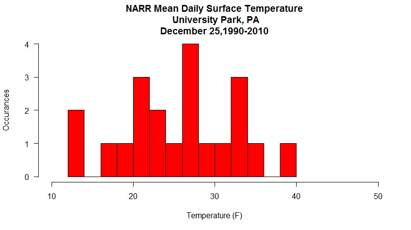
Let's consider the problem that we want to retrieve the Christmas Day mean surface temperatures for University Park, PA for the years 1990 through 2010. How might we do that in an automated manner? Let's look at some code... (Don't forget to set your working directory!)
# if for some reason we need to reinstall the
# package, then do so.

if (!require("ncdf4")) {
  install.packages("ncdf4") }

library(ncdf4)

# specify the file name and location URL
filename<-"air.sfc.1990.nc"
saved_filename<-"air.sfc.1990mean.nc"
url <- "ftp://ftp.cdc.noaa.gov/Datasets/NARR/Dailies/monolevel/"

# get the file... the mode MUST be "wb" (write binary)
download.file(paste0(url,filename), saved_filename, quiet = FALSE, mode="wb")

# open the file
nc <- nc_open(saved_filename)

# print some info to show a good retrieval
print(head(nc$dim$time$vals))

# close the file
nc_close(nc)

# delete the file (this is optional)
file.remove(saved_filename)
Notice in this code we send the filename and its location to a function: download.file(...) which fetches the file and places it in your working directory (as a default). There are numerous parameters that can be set but notice that you can control the saved file name as well as the appearance of the progress bar via the quiet parameter. In fact, we can get quite fancy here if we want. For example, I can create a sub-directory (manually) named "data" within the working directory where I can store the data files that I download (by adding "data/" to the saved file name). I can also check to see if the file I want to download already exists in my directory by using the file.exists(...) function. See the modified code snippet below that only downloads the file if it doesn't exist in the "data/" subdirectory. Note that I have commented out the file.remove(saved_filename) command at the end of the script. In this context (and for the sake of speed) I want to keep the files that I download, but when I run the script for real, I will delete them to save space (it will take much longer to run the script though).
filename<-"air.sfc.1990.nc"
saved_filename<-"data/air.sfc.1990.nc"
url <- "ftp://ftp.cdc.noaa.gov/Datasets/NARR/Dailies/monolevel/"

# get the file... the mode MUST be "wb" (write binary)
if(!file.exists(saved_filename)) {
    download.file(paste0(url,filename), saved_filename, quiet = FALSE, mode="wb")
}
Are you getting a feel for where this is going? If we could create a list of filenames to retrieve then we could loop over those names and retrieve the information we need for each year. This is easy and can be accomplished by these three lines located right after the library call...
dates<-seq(1990,2010,1)
in_file_list<-paste0("air.sfc.",dates,".nc")
out_file_list<-paste0("air.sfc.",dates,"mean.nc")
Run these three lines of code and look at the variables in_file_list and out_file_list in the environment inspector. Easy, right? Now, we need the automation part... do you remember how to do it? We put everything that we want to automate and place it in a function. Then we run the command: mapply(...) with the function name and the variables we want to send the function. Here are the basics...
# ALL THE HEADER STUFF GOES HERE

# get our list of dates (keep the list short for testing)
dates<-seq(1990,1992,1)
in_file_list<-paste0("air.sfc.",dates,".nc")
out_file_list<-paste0("air.sfc.",dates,"mean.nc")
url <- "ftp://ftp.cdc.noaa.gov/Datasets/NARR/Dailies/monolevel/"

# make a placeholder for the specific point data we want
narr.timeseries <- data.frame()

# make the retrieve function
retrieve_data <- function(filename, saved_filename) {
  #
  # PUT ALL THE AUTOMATION STUFF IN HERE
  #
}

# call the automation function with the in and out file lists
mapply (retrieve_data, in_file_list, out_file_list)

# ALL THE PLOT STUFF GOES HERE
All that's left is for you to build the data retrieval code in the automation section and add a plot function after the mapply(...). Can you do it? You've done all the pieces before, and there's a small issue or two to sort out... but give it a try. My version of the Christmas daily mean temperatures histogram is below. If you get stuck, I have put my complete copy of the code in the Quiz Yourself section.
Quiz Yourself...
Were you able to figure everything out? If not, click on the bar below to reveal my complete code. Remember (yes, I forgot) that inside of the automation function all of the variables disappear every time the function restarts. If you want to access a variable after the function finished (called a global variable), you must use the "<<-" assignment operator, not just "<-".
# if for some reason we need to reinstall the
# package, then do so.

if (!require("ncdf4")) {
  install.packages("ncdf4") }

library(ncdf4)

# Set up my date range and file info
dates<-seq(1990,2010,1)
in_file_list<-paste0("air.sfc.",dates,".nc")
out_file_list<-paste0("data/air.sfc.",dates,"mean.nc")
url <- "ftp://ftp.cdc.noaa.gov/Datasets/NARR/Dailies/monolevel/"

# choose a day and location
target_datetime<-"12-25"
location<-c(40.85, -77.85)

# This will be our placeholder for the specific point data we want
narr.timeseries <- data.frame()

# we are going to only compute the cloest_point once,
# so let's delete any old versions.
if (exists("closest_point")) { rm(closest_point) }

retrieve_data <- function(filename, saved_filename) {

# get the file
if(!file.exists(saved_filename)) {
  print(paste0("Retrieving <", filename, "> ... Saving <",saved_filename, ">"))
    download.file(paste0(url,filename), saved_filename, quiet = TRUE, mode="wb")
}

  # open the file
  nc <- nc_open(saved_filename)
  data_dims<-nc$var$air$varsize

  #Get the properly formatted date strings/target time index
  ncdates<-nc$dim$time$vals  #hours since 1800-1-1
  origin<-as.POSIXct('1800-01-01 00:00:00', tz = 'UTC')
  ncdates<-origin + ncdates*(60*60)

  # time_index may change due to leap days so we have to calulate it every time
  time_index<-which(strftime(ncdates,format="%m-%d")==target_datetime)

  # lat and lon index will not change, let's find it only once
  if (!exists("closest_point")) {
    lats<-ncvar_get(nc, varid = 'lat',
                     start = c(1,1),
                     count = c(data_dims[1],data_dims[2]))

    lons<-ncvar_get(nc, varid = 'lon',
                     start = c(1,1),
                     count = c(data_dims[1],data_dims[2]))
    lons<-ifelse(lons>0,lons-360,lons)

    distance<-(lats-location[1])**2+(lons-location[2])**2

  # I want closest_point defined outside of the function (global) so I used <<-
    closest_point<<-which(distance==min(distance), arr.ind = TRUE)
  }

  temp_out<-array(data = NA, dim = c(1,1,1))

  temp_out[,,]<-ncvar_get(nc, varid = 'air',
                            start = c(closest_point[1],closest_point[2],time_index),
                            count = c(1,1,1))
  temp_out[,,]<-(temp_out[,,]-273.15)*9/5+32

  # add the row to the data frame
  row <- data.frame(Year=strftime(ncdates[time_index], format="%Y"), Temperature=temp_out[1,1,1])

  # use the global variable
  narr.timeseries <<- rbind(narr.timeseries,row)

  # close the file
  nc_close(nc)

  # delete the file (optional)
  file.remove(saved_filename)

}

# The main loop
mapply (retrieve_data, in_file_list, out_file_list)

# Write the data out to a file (just so we don't have to calculate it again
write.csv(narr.timeseries, "data/christmas_temps.csv")

# converts $Year from a factor to a number
# need this if you want a line/scatter plot
narr.timeseries$Year<-as.numeric(levels(narr.timeseries$Year))[narr.timeseries$Year]

# I think a histogram makes more sense here than a line/scatter plot
hist(narr.timeseries$Temperature,
     ylab = "Occurances", xlab = "Temperature (F)",
     main = paste0("NARR Mean Daily Surface Temperature\n University Park, PA\n",
            "December 25,", head(narr.timeseries$Year,1),"-",tail(narr.timeseries$Year,1)),
     las=1,
     breaks=10,
     col="red",
     xlim=c(10,50)
)