To GRIB or not to GRIB

Explore Further...

As I mentioned in the beginning of this lesson, the "raw"-est form of environmental data you'll run across is likely to be the WMO standard GRIdded Binary (GRIB) data. I say "raw" because GRIB files were not created with the casual end-user in mind. The GRIB format was created for transmitting large volumes of gridded data via computer-to-computer communications. GRIB also serves as an efficient storage and retrieval data format and is specially designed for use in autonomous systems. What this all means for you and me is that we are not meant to be rooting around inside GRIB files (Is it a secret club?... maybe). If you are so inclined, peruse the GRIB User's Guide. However, don't delve too deeply because we are going to get some tools to help us decode the raw files into something more meaningful.

We will explore two possible approaches for reading GRIB files. Both involve installing other tools to decode the files and convert them into something more meaningful.

Method 1: WGRIB/WGRIB2

The first place I started looking was R libraries to handle GRIB files. There are some out there, and you are welcome to play around with them (rNomads even has some built-in GRIB functions). Many of these R libraries, however, are merely wrappers that execute exterior tools (and to make matters worse, I found significant compatibility issues when trying to run pre-built commands). That said, I was able to read and plot GRIB files from the NARR. Let me show you how.

First, we need some data to play with. The GRIB versions of the NARR are hosted by the NCAR/UCAR Research Data Archive. In fact, there are many different types of data housed at this site (feel free to browse). You will need to register but the account is free, so go ahead and do that now. After you are registered, proceed to the NARR page and after reading about the data set, click on the "Data Access" tab and then on the "regrouped 3-hourly files". To start, go to "Faceted Browse", then pick a single date before hitting continue. On the next page, select "Temperature" from the parameter list, and "Ground or water surface" from the level list. Click on the "Update the List" button and then select one of the files below (it doesn't really matter for our example... each file spans 10 days). Download the compressed ".tar" file and extract the contents in your target directory. You should have a directory of filenames that look like "merged_AWIP32.2017030100.RS.sfc". Copy one of those files to your R-script directory (just to make it easy).

Now that we have the data, we need to get the tools that will actually process the GRIB files. We are going to use the Climate Prediction Center's WGRIB and WGRIB2 decoders. Start by going to the WGRIB website and finding the instructions for your operating system. Windows users can get pre-compiled (exe's and dll's); Mac users will need to compile their own. For Windows users (of which I am one), you need to place all of the pre-compiled WGRIB files in a directory (I placed it under "Program Files") and then add that directory to your system path (if you don't know how to do that, just Google it). Now do the same for WGRIB2 by starting at the CPC's WGRIB2 website. You should know that it works when you can type "wgrib" or "wgrib2" in a command window and get a display of the usage instructions (see a picture of mine).

I should point out that there are two different formats for GRIB files. The older one, GRIB1 or just GRIB, and the newer one GRIB2. You must use the proper form of WGRIB/WGRIB2 depending on the file that you want to decode (newer files tend to be GRIB2), but some systems like the NARR still use the older GRIB format (for compatibility, I suspect). Generally, the site you download from will tell you, but you'll know if you are using the wrong command if you get a "not in GRIB format" type of error. If you stumble upon files in a GRIB2 format, it's an easy fix, you just have to replace wgrib with wgrib2 for all of the code below.

Whew! The good news is that we are over the hump in terms of the technical stuff. Now, let's plot the data. Open a new R-script, and enter the following lines of code:

# set the file name
grib.file<-"merged_AWIP32.2017030100.RS.sfc"

# query the GRIB file for the headers
file.info<-shell(paste0("wgrib -s ", grib.file), shell=NULL, flag="", intern = TRUE, wait = TRUE)

These three lines first define a file name and variable name. Then we run the external program wgrib command using R's shell(...) function. Basically, this function is the same as running wgrib -s merged_AWIP32.2017030100.RS.sfc from a command prompt window, except we can capture the result and paste it into the R-object: file.info. Take a look at file.info... it's a listing of the file's record headers. To interpret them, you can read WGRIB's user's guide. The important thing to note is the variable and level information stored in each record. Now we can run the next four commands in our script:

# specify the variable/level I want
var<-"TMP:sfc"

# run wgrib decoding the proper record and write output file
shell(paste0("wgrib -d ", grep(var, file.info), " -text -o wgrib_output.txt ", grib.file), shell=NULL, flag="", intern = TRUE, wait = TRUE)

# read the output file into R
values<-read.csv("wgrib_output.txt")

# delete the output file (we don't need it anymore)
file.remove("wgrib_output.txt")

First, we define the variable string we want (by browsing the file.info table). Note that if we already know what we want, there's no need to even collect file info at all. Next, we run a shell command again telling wgrib that we want to decode "-d" the record number containing the variable string (that's what grep(...) gives us). We want the output to be "-text" and the output to be sent to "wgrib_output.txt".  All that's left to do is read in the output file and then delete it (because we don't need it anymore). The variable values is a data frame with a single column of numbers rather than a grid, so now we need to fix that before we plot it.

# Replace the missing value: 999999 with NA
values$X349.277[which(values$X349.277>500)]<-NA

# convert from K to degrees F
values$X349.277<-(values$X349.277-273.15)*9/5+32

# make the single column into a matrix (grid)
grid=matrix(values$X349.277, nrow=349, ncol=277)

So how do we know how many rows and columns the data are? And even more important, what are the latitudes and longitudes of each point? These GRIB data grids don't contain any specific spatial information because it is assumed that you know this already. So how do we figure this out? First, we know from previous explorations that NARR data is generated on a 349x277 grid with a Lambert conformal projection. We know this from the NARR documentation and also from a more thorough investigation of the GRIB header information (try: wgrib -V merged_AWIP32.2017030100.RS.sfc and see what you get.). Furthermore, we previously generated the lat/lon grids from one of the NetCDF files. You can run one of these scripts again to strip out the lat and lon from the NetCDF files, or you can simply create an R-data object that contains those variables. I saved those two lat/lon grids as an R-object that you can just load into your current script. Copy this file: narr_lats_lons.RData into your working directory and add the line: load("narr_lats_lons.RData") to the top of your script. Notice when you source the script, variables lats and lons now appear in the Environment tab. 

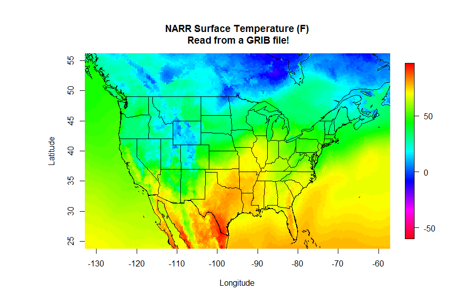
Finally, you can read the latitude and longitude in from another GRIB file. This file contains all of the constant fields of the NARR such as the elevation, soil type and lat/lon of each grid point (you want to grab the file named "rr-fixed.grb". You can read in these fields just as you did the temperature data and then make your plot. Give it a try, you should have all the pieces to produce the plot below. Start with the NetCDF plotting code and swap the GRIB lines. If you need a hint, click below to reveal the code (one for reading the lat/lon values and one for reading and plotting the NARR data).

North American Regional R analysis data from March 1, 2017. This data was retrieved from the UCAR/NCAR GRIB archive, then decoded and plotted in R.

Credit: UCAR/NCAR Research Data Archive (plot by David Babb)

# THIS SCRIPT READS IN THE FIXED VALUES GRIB
# FILE TO RETRIEVE THE LATITUDE AND LONG GRIDS

# set the file name
grib.file<-"rr-fixed.grb"

# specify the latitude variable
var<-"NLAT:sfc"

# query the GRIB file for the headers
file.info<-shell(paste0("wgrib -s ", grib.file), shell=NULL, flag="", intern = TRUE, wait = TRUE)

# run wgrib decoding the latitudes and write output file
shell(paste0("wgrib -d ", grep(var, file.info), " -text -o wgrib_output.txt ", grib.file), shell=NULL, flag="", intern = TRUE, wait = TRUE)

# read the output file into R
grib_lats<-read.csv("wgrib_output.txt")

# delete the output file (we don't need it any more)
file.remove("wgrib_output.txt")

# specify the longitude variable
var<-"ELON:sfc"

# run wgrib decoding longitude and write output file
shell(paste0("wgrib -d ", grep(var, file.info), " -text -o wgrib_output.txt ", grib.file), shell=NULL, flag="", intern = TRUE, wait = TRUE)

# read the output file into R and delete it
grib_lons<-read.csv("wgrib_output.txt")
file.remove("wgrib_output.txt")

# make the single columns into matrices (grid)
grid_lats=matrix(grib_lats$X349.277, nrow=349, ncol=277)
grid_lons=matrix(grib_lons$X349.277, nrow=349, ncol=277)

# swap the longitudes for the map routine
grid_lons<-grid_lons-360

# remove the objects that we don't need anymore
rm(grib_lats, grib_lons)

# THIS SCRIPT READS NARR DATA FROM A GRIB FILE

# We'll need these libraries for plotting
library(fields)
library(maps)

# Read and process the lat/lon script first
source("read_lat_lon.R")

# set the file name
grib.file<-"merged_AWIP32.2017030100.RS.sfc"

# query the GRIB file for the headers
file.info<-shell(paste0("wgrib -s ", grib.file), shell=NULL, flag="", intern = TRUE, wait = TRUE)

# specify the variable/level I want
var<-"TMP:sfc"

# run wgrib decoding the proper record and write output file
shell(paste0("wgrib -d ", grep(var, file.info), " -text -o wgrib_output.txt ", grib.file), shell=NULL, flag="", intern = TRUE, wait = TRUE)

# read the output file into R
values<-read.csv("wgrib_output.txt")

# delete the output file (we don't need it any more)
file.remove("wgrib_output.txt")

# Replace the missing value: 9.99E+20 with NA
values$X349.277[which(values$X349.277>50000)]<-NA

# convert from K to degrees F
values$X349.277<-(values$X349.277-273.15)*9/5+32

# make the single column into a matrix (grid)
grid=matrix(values$X349.277, nrow=349, ncol=277)

# plot the data
colormap<-rev(rainbow(100))

# Note: Remember, if you get an error that says, "plot too large"
# either expand your plot window, or reduce the "pin" values
par(pin=c(6.25,4))

image.plot(grid_lons, grid_lats, grid, col = colormap,
           xlim=c(-130,-60), ylim=c(25,55),
           xlab = "Longitude", ylab = "Latitude",
           main = "NARR Surface Temperature (F)\n Read from a GRIB file!")

# draw the map
map('state', fill = FALSE, col = "black", add=TRUE)
map('world', fill = FALSE, col = "black", add=TRUE)

Method 2: DEGRIB

We saw in the first method that R has no native functions that can decode GRIB files, and thus we need to interface with some tools to help up do so. We were able to use R to automate the calling of either "wgrib.exe" or "wgrib2.exe" by using the shell command. The output of these GRIB decoders is fed into a file which is then read back into R. The advantage of this method is that many operations can be automated, extracting and analyzing large quantities of data. However, technical considerations may limit the effectiveness of this approach.

A second method is to first decode the GRIB files manually into a format better suited for R. This method also uses a third-party tool but is not called by the R program. Its implementation is far more straightforward (in most cases) but in my opinion less powerful because of the lack of automation available. The utility that we are going to use is called DEGRIB and is available from the Meteorological Development Laboratory of the National Weather Service. It was initially developed for decoding output from the National Forecast Database. However, it is a great tool for decoding both GRIB1 and GRIB2 files. Start with the installation instructions... if you have Windows or Linux, the process is relatively simple (with a Mac, it may be more complex). You eventually want to run the program "tkdegrib.exe".

Once in the program, select the "GIS" tab and then use the top portion of the GUI window to navigate to the proper folder/file. The file details appear in the middle section of where you can choose one of the records to decode. Finally, choose an export method (lower-left... I recommend either .csv or NetCDF) and adjust your precision and units in the lower right and generate your file. You can now load this file into R using the methods that you already know. One advantage of this method is that you also get latitude and longitude columns along with your selected data. Give it a try if you like!