5.4.1.3: Stabilized Flow of Gas to a Vertical Production Well in Terms of the Real Gas Pseudo-Pressure, m(p)

In the two previous developments of the stabilized inflow performance relationship for gas (in terms of pressure and the pressure-squared), we made simplifying assumptions on the pressure dependency of the group, $\frac{p}{{\mu }_{g}Z}$. I stated that within certain pressure ranges these assumptions were valid. However, there may be cases where these assumptions are not valid over the entire pressure range of interest. In these cases, we need to develop a general equation that is valid for all pressures. We can achieve this with the Real Gas Pseudo-Pressure Formulation. We define the real gas pseudo-pressure, $m\left(p\right)$, as:

The terminology, $m\left(p\right)$ , implies that the real gas pseudo-pressure is a function of pressure. The units of $m\left(p\right)$ are $ps{i}^2/cp$. We can see from Equation 5.19 that:

or,

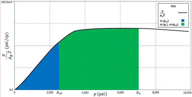
The relationships expressed in Equation 5.20 are illustrated in Figure 5.01. In this figure, $\frac{p}{{\mu }_{g}Z}$, is plotted on the y-axis and $p$ is plotted on the x-axis. The blue area under the curve represents $\frac{m\left(p_{wf}\right)}{2}={\displaystyle {\int }_{14.7}^{p_{wf}}\frac{p}{{\mu }_{g}Z}}dp$ while the total area (blue plus green areas) under the curve represents $\frac{m\left(p_e\right)}{2}={\displaystyle {\int }_{14.7}^{p_e}\frac{p}{{\mu }_{g}Z}}dp$. These are two of the integrals in Equation 5.20. The green area under the curve then represents $\frac{\left[m\left(p_e\right)-m\left(p_{wf}\right)\right]}{2}={\displaystyle {\int }_{p_{wf}}^{p_e}\frac{p}{{\mu }_{g}Z}}dp$.

Substituting Equation 5.20b into Equation 5.10 results in:

Performing the integration on the left-hand side of Equation 5.21 results in:

Rearranging Equation 5.22 results in:

or,

or, after substituting the normal U.S. definitions of $p_{SC}$ and $T_{SC}$ :

The only thing remaining for the pseudo-pressure formulation is the construction of the $m\left(p\right)$ function. To do this, we perform numerical integration on the $\frac{p}{{\mu }_{g}Z}$ function. There are many ways to perform numerical integration; however, one of the most common methods is to approximate the area under the curve with a series of rectangles and to sum the areas of these rectangles. This is illustrated in Figure 5.02.

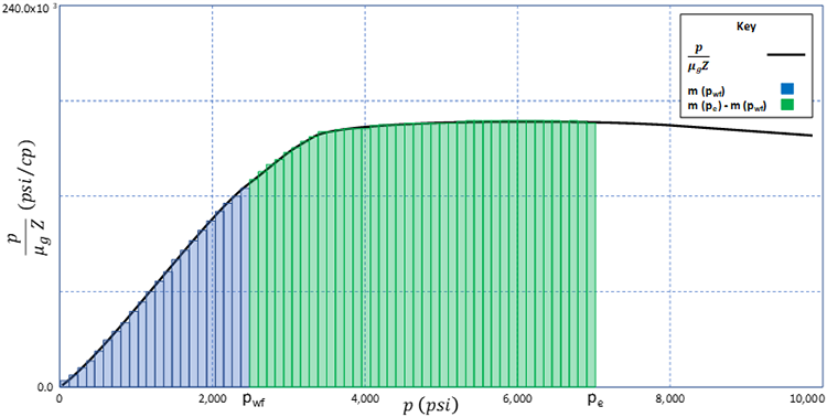
Using this approach, we can approximate the integral (area under the curve) with:

The Real Gas Pseudo-Pressure Formulation is the most rigorous and general formulation for the inflow performance relationship for gas and is valid over all pressure ranges. Even in pressure ranges where another formulation may be valid, the real gas pseudo-pressure formulation is more rigorous.

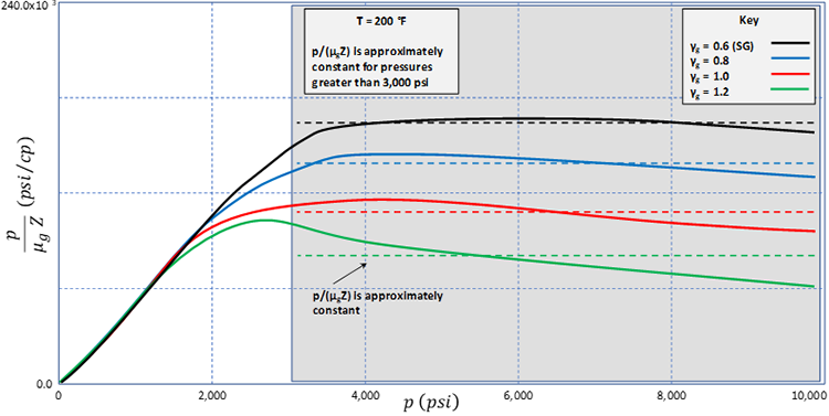
As I just mentioned, there are pressure ranges where the Pressure Formulation and the Pressure-Squared Formulation are valid. If we were to plot the $\frac{p}{{\mu }_{g}Z}$ group (on the y-axis) versus $p$ on the x-axis, then we would develop the plot shown in Figure 5.03. This plot illustrates that the $\frac{p}{{\mu }_{g}Z}$ group is approximately constant for p > 3,000 psi and that the Pressure Formulation is valid when all pressures in the pressure range of interest are greater than 3,000 psi.

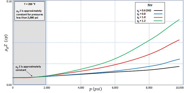
We can also plot ${\mu }_{g}Z$ (on the y-axis) versus $p$ on the x-axis to develop the plot shown in Figure 5.04. This plot illustrates that the ${\mu }_{g}Z$ product is approximately constant for p < 2,000 and that the Pressure-Squared Formulation is valid when all pressures are less than 2,000 psi.