5.5.1: Field and Well Performance of Gas Reservoirs by Material Balance

Volumetric Gas Reservoirs

We were introduced to the concept of material balance in Lesson 4 when we discussed oil reservoirs. In this section, we will discuss the material balance method for Volumetric Gas Reservoirs (reservoirs where the pore-volume occupied by the gas remains constant with time and pressure depletion). We can approach the development of the material balance method from the perspective of the Volumetric Method, as we did in Lesson 4 for oil reservoirs, or from the perspective of the Real Gas Law. I will discuss both of these perspectives in this lesson.

From the perspective of the Volumetric Method for estimating in-place fluids, from Equation 5.01, we know that the original gas-in-place:

As I did for oil reservoirs, I simplified this version of the equation (from Equation 5.01) by assuming that the bulk volume $V_b$, is in bbls and is based on the net rock volume (that is, the net-to-gross ratio and the unit conversion constant, 5.615 ft³/bbl, have already been applied). I also assumed that the water saturation is at its minimum value of $\overline{S_{wir}}$.

Equation 5.44 is valid for any pressure conditions. In the Volumetric Method for OGIP estimation discussed earlier, all of the pressure dependent properties are evaluated at the initial reservoir pressure. If we evaluate Equation 5.44 twice, once at the initial conditions and once at some arbitrary, future condition ($G\text{'}$), then we would have:

and

Where $\overline{B_{gi}}$ and $\overline{B_g}$ are in bbl/SCF (Equation 5.09b). Subtracting Equation 5.45b from Equation 4.45a results in:

$\Delta G$ in this equation is the change in the gas-in-place (SCF) in the reservoir from the initial condition to the future condition. Now, from material balance (mass is neither created nor destroyed), this change in mass is due to the expansion of the gas and must be equal to the mass of the cumulative gas produced from the wells during the time period, $G_p$:

To make Equation 5.47 more convenient, we can substitute Equation 5.45a back into the equation:

or after multiplying both sides by the gas formation volume factor, $\overline{B_g}$, and rearranging:

Where:

• $G$ is the original-gas-in-place, OGIP, SCF
• $G\text{'}$ is the current-gas-in-place, CGIP, at a future date, SCF
• $V_b$ is the net rock volume, bbl
• $\overline{\varphi }$ is the porosity averaged over the reservoir, fraction
• $\overline{S_{wir}}$ is the irreducible water saturation averaged over the reservoir, fraction
• $\overline{B_{gi}}$ is the initial gas formation volume factor averaged over the reservoir, bbl/SCF
• $\overline{B_g}$ is the gas formation volume at a future time averaged over the reservoir, bbl/SCF
• $\Delta G$ is the change in gas-in-place, SCF
• $G_p$ is the gas production, SCF

This is the derivation of the Material Balance Equation for volumetric reservoirs containing a natural gas. In this equation, the left-hand side represents the reservoir barrels of natural gas removed from the reservoir through the production wells, while the right-hand side represents the expansion of natural gas in the reservoir. From the perspective of the Volumetric Equation (Equation 5.01), the Material Balance method states that the standard cubic feet of gas produced through the wells must equal the change in standard cubic feet in the pore-volume of the reservoir.

As I mentioned earlier, we can also look at the material balance method from the perspective of the Real Gas Law:

We start with a lb-mol balance in the reservoir where the lb-mols produced from the reservoir, $n_p$, must equal the lb-mols initially in the reservoir, $n_i$ minus the lb-mols currently in the reservoir, $n_r$,:

Substituting the appropriate conditions on these quantities (standard conditions for $n_p$, initial reservoir conditions for $n_i$, and current reservoir conditions for $n_r$), we have:

In this equation, I used the definition of a Volumetric Reservoir (time invariant pore-volume) to remove the volume occupied by the gas from the parenthesis on the right-hand side of the equation. The unit conversion constant of 5.615 ft³/bbl was required because the units of $V_b$ are in barrels. Dividing by $\frac{p_{SC}}{Z_{SC}R{T}_{SC}}$ results in:

Factoring $\frac{\overline{p_i}}{Z_i}$ from the parenthesis results in:

Finally, noting that $\frac{5.615Z_{SC}{T}_{SC}}{T_r{p}_{SC}}\frac{\overline{p_{\iota }}}{Z_i}$ is the reciprocal of the initial gas phase formation volume factor, ${\mathit{B}}_{gi}\left({\mathit{B}}_g\text{ in bbl/SCF}\right)$, and that $\frac{5.615V_b\overline{\varphi }\left(1.0-\overline{S_{wir}}\right)Z_{SC}{T}_{SC}}{T_r{p}_{SC}}\frac{\overline{p_{\iota }}}{Z_i}$ is the original-gas-in-place, $G$ :

or,

Note that we could have easily substituted the definitions of the gas phase formation volume factors into Equation 5.52 to obtain Equation 5.48b. Also note that Equation 5.53c is the equation of a straight line with $\frac{p_r}{Z_r}$ on the y-axis and $G_p$ on the x-axis. This is illustrated in Figure 5.06.

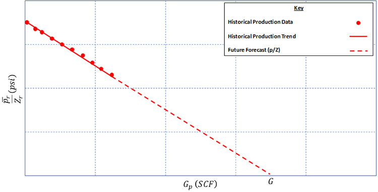
As with material balance for oil reservoirs, this equation and its plot can be used to make an estimate of the OGIP or to make future reservoir forecasts. We can estimate a future forecast of the volume produced, $G_p$, at any reservoir pressure, $\overline{p_r}$, by simply dividing the pressure of interest by its corresponding Z-factor and looking up the cumulative gas produced, $G_p$, at that $\frac{\overline{p_r}}{Z_r}$ value from the $p/Z\text{ Plot}$. For estimating the OGIP, we can see from Equation 5.53c, that the x-intercept ($\frac{\overline{p_r}}{Z_r}=0$) occurs when $G=G_p$. Therefore, we can look at the x-intercept of the $p/Z\text{ Plot}$ to estimate the OGIP, $G$, directly.

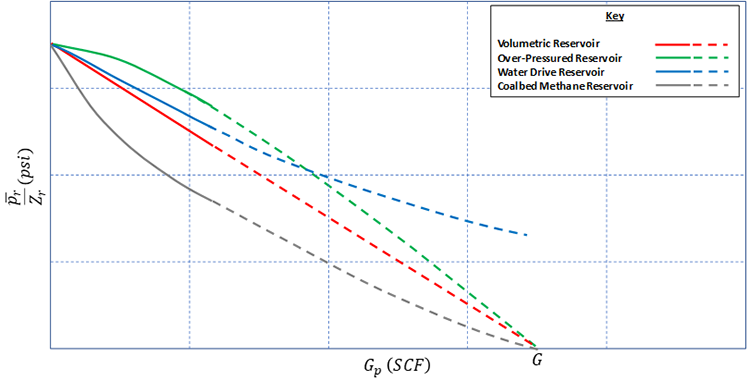
In addition, we can use the $p/Z\text{ Plot}$ as a diagnostic plot to help us identify the type of reservoir we are working with. Figure 5.07 shows common reservoir types on a $p/Z\text{ Plot}$.

Getting back to Equation 5.48b, we can also use it to estimate the original-gas-in-place and to make future forecasts. This is done by redefining terms in Equation 5.48b.

Where:

• $F$ is the sum of all Flow (production) from the reservoir, bbl
• $G$ is the original-gas-in-place, SCF
• $E_t$ is the total Expansion of the system, bbl/SCF

Note that Equation 5.54 for gas is identical to Equation 4.66 from Lesson 4 for oil with the exception that the original-gas-in-place, $G$ , replaces the original-oil-in-place, $N$.

When we include additional derive mechanisms into our material balance equation, we can rewrite Equation 5.54 as:

This equation is identical to Equation 4.67 from Lesson 4 for oil reservoirs with the exception that the original-gas-in-place is substituted for the original-oil-in-place. The entries in Equation 5.55 are listed in Table 5.02.

Table 5.02: Material Balance Equation for Gas in Terms of Rock and Fluid Properties

Term	Description
$F=G_p{B}_g+W_p\overline{B_w}$	Total volume of withdrawal (production) at reservoir conditions in bbl
$G_p{B}_g$	Cumulative gas production in bbl
$W_p\overline{B_w}$	Cumulative water production in bbl
$E_t=E_g+\overline{B_{gi}}{E}_{fw}$	Total expansion in the reservoir in bbl/SCF
$E_g=\left(\overline{B_g}-\overline{B_{gi}}\right)$	Total expansion of the gas, bbl/SCF
$E_{fw}=\frac{\overline{S_{wir}}{c}_w+c_{PV}}{\left(1.0-\overline{S_{wir}}\right)}\left(p_i-\overline{p}\right)$	In over-pressured reservoirs, the expansion of the water and rock may add appreciable energy to the system, dimensionless
$W_e\overline{B_w}$	If the reservoir is connected to an active aquifer, then once the pressure drop is communicated throughout the reservoir, the water will migrate into the reservoir resulting in a net water encroachment, We, bbl

Where:

• $G$ is the original-gas-in-place, SCF
• $G_p$ is the gas production, SCF
• $\overline{B_{gi}}$ is the initial gas phase formation volume factor averaged over the reservoir, bbl/SCF
• $\overline{B_g}$ is the gas phase formation volume at a future time averaged over the reservoir, bbl/SCF
• $V_b$ is the net rock volume, bbl
• $\overline{\varphi }$ is the current porosity averaged over the reservoir, fraction
• $\overline{S_{wir}}$ is the irreducible water saturation averaged over the reservoir, fraction
• $c_w$ is the water compressibility, 1/psi
• $c_{PV}$ is the rock pore-volume compressibility, 1/psi
• $\overline{p}$ is the current pressure averaged over the reservoir, psi
• $p_i$ is the current pressure averaged over the reservoir, psi

Since Equation 5.55 is a direct counterpart to the oil material balance equation, all of the analysis techniques discussed in Lesson 4 for oil reservoirs are applicable to gas reservoirs.