Lesson 5: Reservoir Engineering for Gas Reservoirs
5.0: Lesson Overview
In this lesson, we will discuss Reservoir Engineering for natural gas reservoirs. The tasks performed by reservoir engineers working on gas fields are much the same as those performed for oilfields. These tasks include estimating the original-gas-in-place, or OGIP, analyzing current production rate and pressure trends from the wells and the reservoir, forecasting future performance from these trends, and determining the economic recovery and the Estimated Ultimate Recovery (EUR) of a well, reservoir, or field.
The main difference between natural gas as a produced phase and oil as a produced phase is the highly compressible nature of gas. In many of the methods we discussed for oil reservoirs, we assumed that the oil phase compressibility obeyed the definition of compressibility for a slightly compressible liquid, Equation 3.47:
Natural gas is a Real Gas, and as such, it will obey the Real Gas Law, Equation 3.27:
The fact that natural gas is a real gas and obeys the Real Gas Law has many significant ramifications to the reservoir engineering tasks that we have discussed. In this lesson, we will use the Real Gas Law to develop our equations for the stabilized inflow performance relationships, the transient diffusivity equation, material balance equation, and decline curve analysis.
Learning Objectives
By the end of this lesson, you should be able to:
- discuss the difference between compressible fluids (gases) and slightly compressible fluids (crude oils);
- discuss two methods of calculating the Original-Gas-in-Place, OGIP, in a gas accumulation;
- calculate the OGIP of a natural gas reservoir using the Volumetric Method and Material Balance Method given appropriate data;
- list and describe the four drive mechanisms associated with gas production;
- calculate the stabilized production rates from a gas production well given the current flow regime and given appropriate data;
- list the three formulations used in the stabilized production rates from a gas production well and the pressure ranges where these formulations are appropriate;
- forecast future production from a natural gas reservoir or production well using the Material Balance Method and Decline Curve Analysis given appropriate data; and
- estimate the economically recoverable gas and Estimated Ultimate Recovery (EUR) from a natural gas reservoir
Lesson 5 Checklist
| To Read | Read the Lesson 5 online material | Click the Introduction link below to continue reading the lesson 5 material |
|---|---|---|
| To Do | Lesson 5 Problem Set | Submit your solutions to the Lesson 5 Problem Set assignment in Canvas |
Please refer to the Calendar in Canvas for specific time frames and due dates.
Questions?
If you have questions, please feel free to post them to the Course Q&A Discussion Board in Canvas. While you are there, feel free to post your own responses if you, too, are able to help a classmate.
5.1: Introduction
In Lesson 3, we discussed basic Rock, Fluid, and Rock-Fluid Interaction properties; while in Lesson 4, we applied these properties to oil reservoirs. In this lesson, we will discuss how these properties are used by reservoir engineers working on gas reservoirs.
The tasks for reservoir engineers working on gas wells or gas fields are much the same as the tasks involved for oilfields: the estimation of the original gas-in-place, OGIP, and the estimation of the rates and volumes of fluids produced from the production wells and from the field. For in-place fluid calculations, the Volumetric Method and the Material Balance Method are just as applicable for gas reservoirs as they are for oil reservoirs. We will see, however, that there are differences in the forms of the equations due to the compressible nature of gas. In addition, we will see that the stabilized Inflow Performance Relationships, IPR, (boundary dominated well production rates from Darcy’s Law) and the time dependent diffusivity equation are also impacted by the compressible nature of the gas.
5.2: Estimation of Original Gas In-Place, OGIP, Using the Volumetric Method
The Volumetric Method for OGIP is essentially the same for gas reservoirs. The method uses static geologic data to determine the volume of the pore space of the reservoir. Once the volume of the pore space is estimated, then the gas formation volume factor, can be used to estimate the OGIP.
By simply using the definition of reservoir volumes, the original-gas-in-place of the reservoir be determined by:
or, equivalently (after applying the Saturation Constant):
Where:
- is the original-gas-in-place of the reservoir, SCF
- is the gross rock volume, ft3
- is the net-to-gross thickness ratio, fraction
- is the average net reservoir thickness, ft
- is the average gross reservoir thickness, ft
- is the average initial gas saturation, fraction
- is the average initial water saturation, fraction
- is the average reservoir porosity, fraction
- is the average formation volume factor of the gas at initial conditions (pri and Tr), ft3/SCF
As with the oil volumetric equation (Equation 4.02), Equation 5.01 is evaluated at initial pressure and saturation conditions because the original in-place volume is the desired result. Also, as with the volumetric oil equation, the net-to-gross ratio in the volumetric gas equation is simply the thickness fraction that converts the total reservoir thickness to the thickness that contributes to hydrocarbon storage and flow in the reservoir. We use thickness to apply the net-to-gross ratio because rock formations are formed as layers during deposition, and we assume that layers of poor-quality rock may be deposited and intermixed with layers of good quality reservoir rock. We can further define the gross rock volume as:
Where:
- is the gross rock volume, ft3
- is a unit conversion constant, ft2/acre
- is the mapped area of the reservoir, acres
- is the average gross reservoir thickness, ft
As with oil reservoirs, the volumetric method for estimating the in-place volumes is also considered to be less accurate than the material balance method. The reason again being the use of all of the averages in Equation 5.01. This can also be improved by the use of the iso-contour technique describe in Lesson 4.
5.3: Drive Mechanisms in Gas Reservoirs
In Lesson 4, we discussed the drive mechanisms associated with oil reservoirs. For gas reservoirs, there are three drive mechanisms that are associated with conventional gas reservoirs and a fourth drive mechanism associated with unconventional gas reservoirs. These are:
- gas expansion (most significant drive mechanism in conventional gas reservoirs);
- gas desorption (may only be present in certain unconventional gas reservoirs);
- rock and fluid expansion (expansion of the reservoir rock and interstitial water – typically only significant in over-pressured gas reservoirs); and
- natural aquifer drive (or water encroachment).
In this list, I make a distinction between Conventional and Unconventional Gas Reservoirs. Conventional gas reservoirs are reservoirs with sufficiently high permeability to allow for production using conventual well technologies. Unconventional reservoirs are reservoirs with low permeabilities that require special production technologies that allow for economic recoveries of gas. Typically, the threshold to define an unconventional gas reservoir is a reservoir with a permeability less than 0.1 md.
Gas expansion is the primary drive mechanism in most conventional gas reservoirs. Again, the analogy of a gas-filled balloon a very appropriate analogy. If a balloon is filled with high pressure gas and the end is opened to the low pressure atmosphere, then gas will expand and exit the balloon. This mechanism is very efficient and commonly results in recoveries as high as 85 percent of the original-gas-in-place.
A drive mechanism that is associated with certain unconventional gas reservoirs is gas desorption. As we have already discussed, unconventional gas reservoirs are reservoirs with permeabilities less than 0.1 md. These unconventional reservoirs include:
- tight oil and gas sandstones or carbonates;
- shale gas and shale oil reservoirs; and
- coal seam methane reservoirs.
The last two of these unconventional gas reservoir types, shale gas reservoirs and coal seam methane reservoirs, have a high content of organic material in the reservoir rock. This organic rich rock material has the ability to Adsorb gas onto its surface (gas stored by adhesion onto the surface). As pressure is depleted, this adsorbed gas is released to the pore-volume of the reservoir by the Desorption Process. This desorption of gas may dominate production from the unconventional gas reservoirs in which it occurs.
Rock and fluid expansion in gas reservoirs is identical to that in oil reservoirs. It occurs due to the slightly compressible nature of the Interstitial (or Connate) Water and the reservoir rock. This expansion adds energy to the reservoir and acts to keep the reservoir pressure higher than it would be otherwise. This expansion mechanism is always dominated by gas expansion and may only be significant in cases of over-pressured reservoirs.
The final drive mechanism associated with conventional gas reservoirs is aquifer drive, or water encroachment. As with oil reservoirs, this drive mechanism occurs when the reservoir is in communication with a water-bearing aquifer. As the reservoir pressure declines, the rock and water in the aquifer expand, and water is expelled from the aquifer and into the reservoir. This encroachment of water into the reservoir provides pressure support.
These last two drive mechanisms may be slightly deceptive as to whether they aid in gas production or not. Both of these methods tend to keep reservoir pressures high; however, the principle drive mechanisms, gas expansion, and gas desorption, rely on pressure depletion. In addition, water encroachment may also result in trapped gas behind the invading water front.
5.4: Performance of Gas Wells
5.4: Performance Gass Wells section of this lesson will cover the following topics:
- 5.4.1: Stabilized Inflow Performance of Gas Wells [1]
- 5.4.1.1: Stabilized Flow of Gas to a Vertical Production Well in Terms of Pressure [2]
- 5.4.1.2: Stabilized Flow of Gas to a Vertical Production Well in Terms of Pressure-Squared [3]
- 5.4.1.3: Stabilized Flow of Gas to a Vertical Production Well in Terms of the Real Gas Pseudo-Pressure, m(p) [4]
- 5.4.1.4: The Rawlins and Schellhardt Backpressure or Deliverability Equation [5]
- 5.4.2: Transient Performance of Gas Wells [6]
- 5.4.2.1: Derivation of the Diffusivity Equation in Radial-Cylindrical Coordinates for Compressible Gas Flow [7]
- 5.4.2.2: The Diffusivity Equation for a Gas in Radial-Cylindrical Coordinates in Terms of Pressure [8]
- 5.4.2.3: The Diffusivity Equation for a Gas in Radial-Cylindrical Coordinates in Terms of Pressure-Squared [9]
- 5.4.2.4: The Diffusivity Equation for a Gas in Radial-Cylindrical Coordinates in Terms of Real Gas Pseodo-Pressure, m(p) [10]
5.4.1: Stabilized Inflow Performance of Gas Wells
We have already discussed, the stabilized production of gas is similar to the flow of oil; however, due to the compressible nature of gas, we must consider the pressure dependencies of the gas properties more rigorously than we did for oil. I will again start with the steady-state inflow performance relationship.
For steady-state analysis, we need to make the following assumptions:
- Flow is steady-state and Darcy’s Law applies and all of the assumptions inherent Darcy’s Law are valid in the system
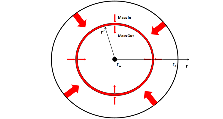
- The drainage volume is radial-cylindrical (see Figure 4.01)
- The drainage volume is bounded in the interior with a cylindrical well (radius equal to ) and kept at flowing well pressure of
- The drainage volume is bounded on the exterior with a cylindrical boundary (radius equal to ) which has an external pressure of
- The drainage volume is bounded on the top and bottom (constant height) no-flow boundaries
- Within the drainage volume, the rock properties are homogeneous (uniform with location)
- Within the drainage volume, the rock properties are isotropic (uniform in all directions)
- Flow is horizontal
With these assumptions, we can use the single-phase version of Darcy’s Law:
In Equation 5.03, we are using the effective permeability to gas in the presence of a water phase to allow for an irreducible, immobile water phase in the reservoir. Now, for radial flow, we have:
Substituting into Darcy’s Law, we have:
Separating variables and integrating results in:
Now, using the assumption of a homogeneous permeability, we have:
To this point, the derivation of the stabilized inflow performance relationship for gas is identical to the derivation for oil. In the derivation of the inflow performance relationship for oil, we assumed that were constant, and we removed them from the integral. As stated earlier, the properties, and , are pressure dependent properties due to the compressible nature of gas and may need to be treated differently from the treatment of the oil properties. These differences manifest themselves in how we treat the integral in Equation 5.08.
There are three methods used in the industry to evaluate the integral in Equation 5.08. These methods lead to three different formulations for the inflow performance relationship for gas. These are:
- Stabilized Production of Gas in Terms of Pressure
- Stabilized Production of Gas in Terms of Pressure-Squared
- Stabilized Production of Gas in Terms of Pseudo-Pressure
In addition to these three analytical inflow performance relationships, we will discuss one common empirical inflow performance relationship, the Rawlins and Schellhardt Backpressure or Deliverability Equation[1].
[1] Rawlins, E.L. and Schellhardt, M.A. 1935. Backpressure Data on Natural Gas Wells and Their Application to Production Practices, 7. Monograph Series, U.S. Bureau of Mines.
5.4.1.1: Stabilized Flow of Gas to a Vertical Production Well in Terms of Pressure
To develop the inflow performance relationships for gas, we will need to use the definition of the gas formation volume factor, , Equation 3.68:
or,
Since Equation 5.08 is written in terms of bbl/day, we need use the form of in bbl/SCF. Substituting Equation 5.09 into Equation 5.08 results in:
Now, if we assume that the term, , is constant with pressure, then we can remove it from the integral (in essence, this is what we did for the oil equation). While at first glance, this may seem like a bad assumption because we are removing p and two pressure dependent functions, and , from an integration with respect to pressure; within certain pressure ranges it is not a bad assumption. This is because we are not interested in how the individual components in the group, , behave with respect to pressure but are concerned with how the group behaves in its entirety. I will discuss this in more detail later in this lesson. If we remove this group from the integral in Equation 5.10, then we obtain:
Performing the two integrations in Equation 5.11:
or,
Rearranging Equation 5.13 results in:
or,
Now, if we use the normal U.S. definitions of Standard Pressure and Standard Temperature , then we have:
Equation 5.14c is the steady-state inflow performance relationship for single-phase gas production. All that remains is to discuss how to evaluate the term, . Typically, we do this by evaluating the average pressure as the arithmetic mean pressure:
and use that average pressure to evaluate and . Because all of the pressure terms in this equation are written directly as , we refer to this formulation as the Inflow Performance Relationship for Gas in Terms of Pressure. As with the oil inflow performance relationship, we can add a skin factor to account for damage or stimulation and write similar equations in terms of (rather than ) for the pseudo steady-state flow regime.
5.4.1.2: Stabilized Flow of Gas to a Vertical Production Well in Terms of Pressure-Squared
To develop the inflow performance relationship in terms of pressure, we assumed that the group, , was relatively constant in the pressure range of interest, and we removed the entire group from the pressure integral in Equation 5.10. In the pressure-squared formulation, we assume that the product is relatively constant with pressure and remove it from Equation 5.10, leaving:
Again, we will see that the product can be safely assumed to be relatively constant over a particular pressure range. Performing both integrations in Equation 5.16 results in:
Rearranging Equation 5.17 results in:
or,
or, after substituting the normal U.S. definitions of and :
In this equation, we evaluate and at the arithmetic mean average pressure, Equation 5.15. Again, we can add a skin factor to account for well damage or stimulation and write similar equations in terms of average pressure for the pseudo-steady state flow regime. Equation 5.18c is the Inflow Performance Relationship for Gas in Terms of Pressure-Squared.
5.4.1.3: Stabilized Flow of Gas to a Vertical Production Well in Terms of the Real Gas Pseudo-Pressure, m(p)
In the two previous developments of the stabilized inflow performance relationship for gas (in terms of pressure and the pressure-squared), we made simplifying assumptions on the pressure dependency of the group, . I stated that within certain pressure ranges these assumptions were valid. However, there may be cases where these assumptions are not valid over the entire pressure range of interest. In these cases, we need to develop a general equation that is valid for all pressures. We can achieve this with the Real Gas Pseudo-Pressure Formulation. We define the real gas pseudo-pressure, , as:
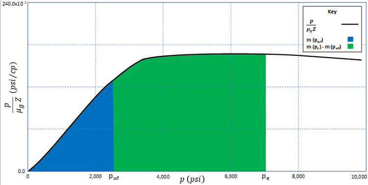
The terminology, , implies that the real gas pseudo-pressure is a function of pressure. The units of are . We can see from Equation 5.19 that:
or,
The relationships expressed in Equation 5.20 are illustrated in Figure 5.01. In this figure, , is plotted on the y-axis and is plotted on the x-axis. The blue area under the curve represents while the total area (blue plus green areas) under the curve represents . These are two of the integrals in Equation 5.20. The green area under the curve then represents .
Substituting Equation 5.20b into Equation 5.10 results in:
Performing the integration on the left-hand side of Equation 5.21 results in:
Rearranging Equation 5.22 results in:
or,
or, after substituting the normal U.S. definitions of and :
The only thing remaining for the pseudo-pressure formulation is the construction of the function. To do this, we perform numerical integration on the function. There are many ways to perform numerical integration; however, one of the most common methods is to approximate the area under the curve with a series of rectangles and to sum the areas of these rectangles. This is illustrated in Figure 5.02.
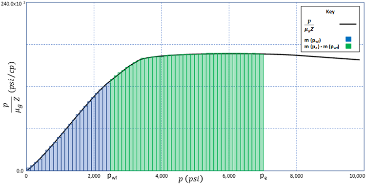
Using this approach, we can approximate the integral (area under the curve) with:
The Real Gas Pseudo-Pressure Formulation is the most rigorous and general formulation for the inflow performance relationship for gas and is valid over all pressure ranges. Even in pressure ranges where another formulation may be valid, the real gas pseudo-pressure formulation is more rigorous.
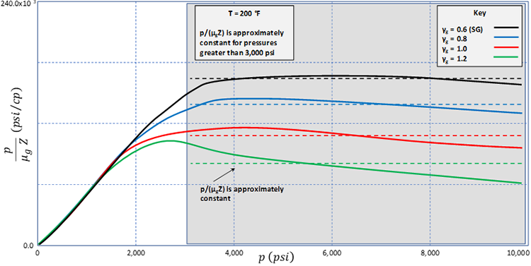
As I just mentioned, there are pressure ranges where the Pressure Formulation and the Pressure-Squared Formulation are valid. If we were to plot the group (on the y-axis) versus on the x-axis, then we would develop the plot shown in Figure 5.03. This plot illustrates that the group is approximately constant for p > 3,000 psi and that the Pressure Formulation is valid when all pressures in the pressure range of interest are greater than 3,000 psi.
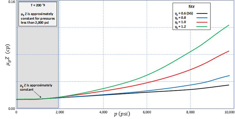
We can also plot (on the y-axis) versus on the x-axis to develop the plot shown in Figure 5.04. This plot illustrates that the product is approximately constant for p < 2,000 and that the Pressure-Squared Formulation is valid when all pressures are less than 2,000 psi.
5.4.1.4: The Rawlins and Schellhardt Backpressure or Deliverability Equation
One final relationship that is often used in the oil and gas industry is the empirical Rawlins and Schellhardt Backpressure or Deliverability Equation[1]. This equation has the form:
As with all observation-based empirical relationships, to use this equation it must be tuned with appropriate data to determine the values of the tuning parameters, and . To do this, the gas well must be produced at several flowing pressures, , and the resulting stabilized rates measured. Once these tests (Deliverability Tests) are performed, the equation parameters, and , are used to fit the equation to the test results. Table 5.01 a-g summarizes all of the Stabilized Inflow Performance Relationships for gas wells discussed to this point.
| In Terms of Pressure including Damage or Stimulation: All pressures greater than 3,000 psi |
||
|---|---|---|
| Steady-State Flow Regime | Pseudo Steady-State Flow Regime | |
| Drawdown | ||
| Productivity Index |
||
| IPR | ||
| In terms of Pressure including Damage or Stimulation: All pressures greater than 3,000 psi |
||
|---|---|---|
| Steady-State Flow Regime | Pseudo Steady-State Flow Regime | |
| Drawdown | ||
| Productivity Index |
||
| IPR | ||
| In terms of Pressure-Squared including Damage or Stimulation: All pressures less than 2,000 psi |
||
|---|---|---|
| Steady-State Flow Regime | Pseudo Steady-State Flow Regime | |
| Drawdown | ||
| Productivity Index |
||
| IPR | ||
| In terms of Pressure-Squared including Damage or Stimulation: All pressures less than 2,000 psi |
||
|---|---|---|
| Steady-State Flow Regime | Pseudo Steady-State Flow Regime | |
| Drawdown | ||
| Productivity Index |
||
| IPR | ||
| In terms of the Real Gas Pseudo-Pressure including Damage or Stimulation: Valid over the entire pressure range |
||
|---|---|---|
| Steady-State Flow Regime | Pseudo Steady-State Flow Regime | |
| Drawdown | ||
| Productivity Index |
||
| IPR | ||
| In terms of the Real Gas Pseudo-Pressure including Damage or Stimulation: Valid over the entire pressure range |
||
|---|---|---|
| Steady-State Flow Regime | Pseudo Steady-State Flow Regime | |
| Drawdown | ||
| Productivity Index |
||
| IPR | ||
| The Rawlins and Schellhardt Backpressure or Deliverability Equation[1] | ||
|---|---|---|
| Steady-State Flow Regime | Pseudo Steady-State Flow Regime | |
| IPR | ||
The following parameters are used in Table 5.01 or in the development of these equations:
- reservoir pressure at the external boundary of the drainage volume, psi
- flowing well pressure, psi
- average reservoir pressure within the drainage volume, psi
- the real gas pseudo-pressure, psi2/cp
- external radius of the drainage volume, ft
- radius of the well, ft
- pressure at standard conditions (14.7 psi in the U.S.A), psi
- temperature at standard conditions (520°R in the U.S.A), °R
- temperature of the reservoir, °R
- effective permeability to gas in the presence of an immobile water phase, md
- thickness of the reservoir, ft
- gas viscosity, cp
- gas super-compressibility factor, dimensionless
- skin factor, dimensionless
- is the oil production rate during the stabilized production period, SCF/day
- factor in Rawlins and Schellhardt Backpressure or Deliverability Equation[1], SCF/(day-psi(2xn))
- exponent in Rawlins and Schellhardt Backpressure or Deliverability Equation[1], dimensionless
- is the oil phase formation volume factor, bbl/SCF
5.4.2: Transient Performance of Gas Wells
In our earlier discussions on the performance of oil wells, we discussed transient (time dependent) flow and the flow regimes encountered during transient flow. These flow regimes also occur in gas wells and are:
- Well dominated flow
- Wellbore storage
- Damage/Stimulation
- Transient flow
- Late transient flow
- Boundary dominated flow
- Steady-state
- Pseudo steady-state
5.4.2.1: Derivation of the Diffusivity Equation in Radial-Cylindrical Coordinates for Compressible Gas Flow
As with the flow of oil, we begin the derivation of diffusivity equation for compressible gas flow with a mass balance on a thin ring or Representative Elemental Volume, REV, in the reservoir as shown in Figure 5.05. This mass balance results in:
We can elaborate on the definitions of terms in Equation 5.26 as:
and,
Where:
- is the gas density, lb/ft3
- is the gas rate, ft3/day
- is the radial coordinate in a radial-cylindrical coordinate system, ft
- is the radius of the representative elemental volume, REV, ft
- is time, days
- is the porosity of the reservoir, fraction
- is the bulk volume of the representative elemental volume, REV, ft3
- is the reservoir thickness, ft
Substituting Equation 5.27 through Equation 5.29 into Equation 5.26 results in:
or,
Dividing by the term results in:
Now, substituting Darcy’s Law, Equation 5.06 with and without the formation volume factor, , (we want the flow rate in reservoir ft3/day not SCF/day). The unit conversion factor of 5.615 ft3/bbl converts Darcy’s Law from bbl/day to ft3/day:
If we assume that the permeability, , and the thickness, , are uniform, then we have:
or,
To this point, the derivation for the compressible gas equation is identical to the derivation for a slightly compressible liquid equation. This derivation will begin to deviate now. Applying the definition of density for a real gas (Equation 3.71):
Equation 5.34 is a direct result of the Real Gas Law. Substituting into Equation 5.33b results in:
or,
or,
Now, we saw in Lesson 3 that for a real gas, the definition of compressibility is (Equation 3.70b):
or,
Substituting into Equation 5.35c results in:
Equation 5.37 is the nonlinear diffusivity equation describing the transient behavior of compressible (real) gases. We say that it is Nonlinear because of the functions of pressure appearing in the equation. In this nonlinear form, we cannot solve the equation analytically (exactly). In order to obtain analytical solutions to this equation, we must first Linearize it. We do this in the same manner as we linearized the stabilized flow equations: by use of the Pressure, the Pressure-Squared, and the Pseudo-Pressure Formulations.
5.4.2.2: The Diffusivity Equation for a Gas in Radial-Cylindrical Coordinates in Terms of Pressure
As we have already seen, in the pressure range of , the group can be considered to be approximately constant. With this simplification, we can remove the group from the spatial derivative on the left-hand side of Equation 5.37 to obtain:
This is the diffusivity equation for real gases in terms pressure, p. While this may at first glance appear to be linearized, it is not. Both the gas compressibility term, , and the gas viscosity term, , are pressure dependent. When using the pressure formulation, we typically evaluate these terms at either the initial pressure condition, , or the average condition, . (Note: other more rigorous methods are available for the evaluation of the product; however, they are beyond the scope of this course.)
5.4.2.3: The Diffusivity Equation for a Gas in Radial-Cylindrical Coordinates in Terms of Pressure-Squared
In the pressure-squared formulation, we assume that the product is constant. We have already seen that this approximation is valid for . With this simplification, Equation 5.37 becomes:
Now, we can use the identity:
or,
Substituting Equation 5.40b into Equation 5.39 results in:
This is the diffusivity equation for real gases in terms pressure-squared, . Again, the product represents a non-linear term which we evaluate at either the initial pressure, , or the average pressure, .
5.4.2.4: The Diffusivity Equation for a Gas in Radial-Cylindrical Coordinates in Terms of Real Gas Pseudo-Pressure, m(p)
Finally, we will investigate the use of the real gas pseudo-pressure in the diffusivity equation. For this, we differentiate the definition of the pseudo-pressure integral, Equation 5.19, using the fundamental theorem of calculus:
or,
Substituting Equation 5.42b into Equation 5.39 results in:
Again, we evaluate the product at either the initial pressure, , or the average pressure, . In this development, we have:
- is an equation constant (5.615 x 0.001127)
- is the radial coordinate in a radial-cylindrical coordinate system, ft
- is the pressure, psi
- is the real gas pseudo-pressure, psi2/cp
- is the porosity of the reservoir, fraction
- is the gas compressibility, 1/psi
- is the gas viscosity, cp
- is the effective permeability to gas, md
- is time, days
5.5: Field Performance of Gas Reservoirs
5.5: Field Performance of Gas Reservoirs section of this lesson will cover the following topics:
5.5.1: Field and Well Performance of Gas Reservoirs by Material Balance
Volumetric Gas Reservoirs
We were introduced to the concept of material balance in Lesson 4 when we discussed oil reservoirs. In this section, we will discuss the material balance method for Volumetric Gas Reservoirs (reservoirs where the pore-volume occupied by the gas remains constant with time and pressure depletion). We can approach the development of the material balance method from the perspective of the Volumetric Method, as we did in Lesson 4 for oil reservoirs, or from the perspective of the Real Gas Law. I will discuss both of these perspectives in this lesson.
From the perspective of the Volumetric Method for estimating in-place fluids, from Equation 5.01, we know that the original gas-in-place:
As I did for oil reservoirs, I simplified this version of the equation (from Equation 5.01) by assuming that the bulk volume , is in bbls and is based on the net rock volume (that is, the net-to-gross ratio and the unit conversion constant, 5.615 ft3/bbl, have already been applied). I also assumed that the water saturation is at its minimum value of .
Equation 5.44 is valid for any pressure conditions. In the Volumetric Method for OGIP estimation discussed earlier, all of the pressure dependent properties are evaluated at the initial reservoir pressure. If we evaluate Equation 5.44 twice, once at the initial conditions and once at some arbitrary, future condition (), then we would have:
and
Where and are in bbl/SCF (Equation 5.09b). Subtracting Equation 5.45b from Equation 4.45a results in:
in this equation is the change in the gas-in-place (SCF) in the reservoir from the initial condition to the future condition. Now, from material balance (mass is neither created nor destroyed), this change in mass is due to the expansion of the gas and must be equal to the mass of the cumulative gas produced from the wells during the time period, :
To make Equation 5.47 more convenient, we can substitute Equation 5.45a back into the equation:
or after multiplying both sides by the gas formation volume factor, , and rearranging:
Where:
- is the original-gas-in-place, OGIP, SCF
- is the current-gas-in-place, CGIP, at a future date, SCF
- is the net rock volume, bbl
- is the porosity averaged over the reservoir, fraction
- is the irreducible water saturation averaged over the reservoir, fraction
- is the initial gas formation volume factor averaged over the reservoir, bbl/SCF
- is the gas formation volume at a future time averaged over the reservoir, bbl/SCF
- is the change in gas-in-place, SCF
- is the gas production, SCF
This is the derivation of the Material Balance Equation for volumetric reservoirs containing a natural gas. In this equation, the left-hand side represents the reservoir barrels of natural gas removed from the reservoir through the production wells, while the right-hand side represents the expansion of natural gas in the reservoir. From the perspective of the Volumetric Equation (Equation 5.01), the Material Balance method states that the standard cubic feet of gas produced through the wells must equal the change in standard cubic feet in the pore-volume of the reservoir.
As I mentioned earlier, we can also look at the material balance method from the perspective of the Real Gas Law:
We start with a lb-mol balance in the reservoir where the lb-mols produced from the reservoir, , must equal the lb-mols initially in the reservoir, minus the lb-mols currently in the reservoir, ,:
Substituting the appropriate conditions on these quantities (standard conditions for , initial reservoir conditions for , and current reservoir conditions for ), we have:
In this equation, I used the definition of a Volumetric Reservoir (time invariant pore-volume) to remove the volume occupied by the gas from the parenthesis on the right-hand side of the equation. The unit conversion constant of 5.615 ft3/bbl was required because the units of are in barrels. Dividing by results in:
Factoring from the parenthesis results in:
Finally, noting that is the reciprocal of the initial gas phase formation volume factor, , and that is the original-gas-in-place, :
or,
Note that we could have easily substituted the definitions of the gas phase formation volume factors into Equation 5.52 to obtain Equation 5.48b. Also note that Equation 5.53c is the equation of a straight line with on the y-axis and on the x-axis. This is illustrated in Figure 5.06.
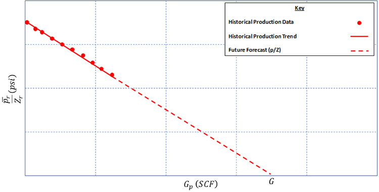
As with material balance for oil reservoirs, this equation and its plot can be used to make an estimate of the OGIP or to make future reservoir forecasts. We can estimate a future forecast of the volume produced, , at any reservoir pressure, , by simply dividing the pressure of interest by its corresponding Z-factor and looking up the cumulative gas produced, , at that value from the . For estimating the OGIP, we can see from Equation 5.53c, that the x-intercept () occurs when . Therefore, we can look at the x-intercept of the to estimate the OGIP, , directly.
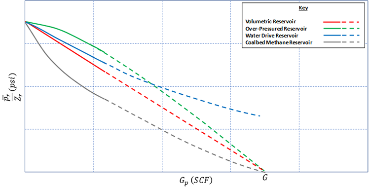
In addition, we can use the as a diagnostic plot to help us identify the type of reservoir we are working with. Figure 5.07 shows common reservoir types on a .
Getting back to Equation 5.48b, we can also use it to estimate the original-gas-in-place and to make future forecasts. This is done by redefining terms in Equation 5.48b.
Where:
- is the sum of all Flow (production) from the reservoir, bbl
- is the original-gas-in-place, SCF
- is the total Expansion of the system, bbl/SCF
Note that Equation 5.54 for gas is identical to Equation 4.66 from Lesson 4 for oil with the exception that the original-gas-in-place, , replaces the original-oil-in-place, .
When we include additional derive mechanisms into our material balance equation, we can rewrite Equation 5.54 as:
This equation is identical to Equation 4.67 from Lesson 4 for oil reservoirs with the exception that the original-gas-in-place is substituted for the original-oil-in-place. The entries in Equation 5.55 are listed in Table 5.02.
| Term | Description |
|---|---|
| Total volume of withdrawal (production) at reservoir conditions in bbl | |
| Cumulative gas production in bbl | |
| Cumulative water production in bbl | |
| Total expansion in the reservoir in bbl/SCF | |
| Total expansion of the gas, bbl/SCF | |
| In over-pressured reservoirs, the expansion of the water and rock may add appreciable energy to the system, dimensionless | |
| If the reservoir is connected to an active aquifer, then once the pressure drop is communicated throughout the reservoir, the water will migrate into the reservoir resulting in a net water encroachment, We, bbl |
Where:
- is the original-gas-in-place, SCF
- is the gas production, SCF
- is the initial gas phase formation volume factor averaged over the reservoir, bbl/SCF
- is the gas phase formation volume at a future time averaged over the reservoir, bbl/SCF
- is the net rock volume, bbl
- is the current porosity averaged over the reservoir, fraction
- is the irreducible water saturation averaged over the reservoir, fraction
- is the water compressibility, 1/psi
- is the rock pore-volume compressibility, 1/psi
- is the current pressure averaged over the reservoir, psi
- is the current pressure averaged over the reservoir, psi
Since Equation 5.55 is a direct counterpart to the oil material balance equation, all of the analysis techniques discussed in Lesson 4 for oil reservoirs are applicable to gas reservoirs.
5.5.2: Field and Well Performance of Gas Reservoirs with Arps Decline Curve Analysis
Since decline curve analysis is an empirical curve fitting / trend-line technique, it can also be used for gas reservoirs with no modifications. We assume that the compressible nature of the gas is built into the established trends. When using Arps[2] Decline Curves, the same assumption applies for gas reservoirs: whatever processes that occurred in the past that helped to establish the trend of the data must continue to occur into the future.
As with oil reservoirs, decline curves for gas reservoirs can be used to make reservoir or well forecasts in both the time and domains, estimate the economic cumulative production from the reservoir or well (given the economic abandonment rate), and estimate the EUR (no economic limit) from the reservoir or well.
[2] Arps, J. J.: “Analysis of Decline Curves,” SPE-945228-G, Trans. of the AIME (1945)
5.6: Key Learnings
- Three of the key tasks performed by reservoir engineers working on a natural gas accumulation are the estimation of the Original-Gas-in-Place, OGIP, in a gas accumulation, the estimation of the stabilized production rate from a vertical production well, and the forecasting of future performance of a gas reservoir or well.
- These tasks have analogs with crude oil reservoirs, but there are significant differences between the methods used to analyze gas reservoirs due to the highly compressible nature of natural gas
- Two common methods for calculating the OGIP in a gas accumulation are:
- The Volumetric Method
- The Material Balance Method
- There are four drive mechanisms in a gas reservoir:
- Gas expansion (most significant drive mechanism in conventional gas reservoirs)
- Gas desorption (may only be present in certain unconventional gas reservoirs)
- Rock and fluid expansion (expansion of the reservoir rock and interstitial water – typically only significant in over-pressured gas reservoirs)
- Natural aquifer drive (or water encroachment)
- The major flow regimes experienced by vertical gas production wells are identical to those experienced by vertical oil production wells. These flow regimes are:
- Well dominated flow
- Transient flow
- Late transient flow
- Boundary dominated flow
- The stabilized production rates from a gas production well occur during the boundary dominated flow regime. These stabilized production rates are governed by the inflow performance relationships.
- The stabilized inflow performance of gas wells and the transient performance of gas wells can be estimated with three formulations. These formulations are based on the manner in which the term, , is integrated. These three formulations are:
- Pressure Formulation: valid for
- Pressure-Squared Formulation: valid for
- Pseudo-Pressure Formulation: valid for all pressures
- The Pseudo-Pressure Formulation is the most rigorous formulation within any pressure range of interest (even if another formulation is valid in that pressure range)
- Two common methods for making future reservoir or well forecasts for gas accumulations are:
- The Material Balance Method
- Decline curve analysis
- Exponential decline
- Hyperbolic decline
- Harmonic decline
5.7: Summary and Final Tasks
Summary
In this lesson, we discussed three very important tasks performed by reservoir engineers working on natural gas reservoirs. These tasks are identical to those performed by reservoir engineers working on oil reservoirs. These are:
- estimation of the Original-Gas-In-Place or OGIP;
- estimation of the stabilized production rate from a vertical gas well; and
- forecasting the future performance of gas reservoir and wells.
We saw that there were two methods commonly used in the oil and gas industry estimating the OGIP:
- the Volumetric Method
- the Material Balance Method
We also discussed that of these two methods, the material balance method is typically assumed to be more accurate as it is based on dynamic data.
We discussed the four Drive Mechanisms associated with gas reservoirs:
- gas expansion (most significant drive mechanism in conventional gas reservoirs)
- gas desorption (may only be present in certain unconventional gas reservoirs)
- rock and fluid expansion (expansion of the reservoir rock and interstitial water – typically only significant in over-pressured gas reservoirs)
- natural aquifer drive (or water encroachment)
We saw that the gas desorption mechanism is only applicable for unconventional gas reservoirs with significant organic content in the rock. The criteria of high organic content in the rock is normally met in:
- coal seam methane reservoirs
- shale gas reservoirs
We also discussed the stabilized production rates from vertical gas production wells. We saw that there were several flow regimes possible in a hydrocarbon reservoir (both natural gas and crude oil) that occurred at different stages in a well’s productive life. In Figure 4.06 from Lesson 4, we saw that these flow regimes occurred sequentially as the pressure disturbance caused by production propagates outward from the well towards the boundaries. These flow regimes are:
- Well dominated flow
- Wellbore storage
- Damage/Stimulation
- Transient flow
- Late transient flow
- Boundary dominated flow
- Steady-state
- Pseudo steady-state
In both gas and oil wells, the initial well dominated flow regime is controlled by well properties and well damage/stimulation, not reservoir properties. The transient flow regime is governed by the diffusivity equation and is characterized by time dependent rates and/or pressures. The onset of the late transient period occurs when the pressure disturbance from the production well reaches the first boundary of the drainage volume. The end of the late transient period occurs when the pressure disturbance reaches the last boundary of the drainage volume. The boundary dominated flow regime is the last flow regime experienced by the well. Stabilized production occurs during the boundary dominated flow period and is described by one of the Inflow Performance Relationships, IPRs that we derived in this lesson.
In natural gas wells, three different formulations can be used to develop the stabilized IPRs and the transient diffusivity equation. These formulations are based on the manner in which the term, , is integrated in the development of the different equations. These three formulations are:
- Pressure Formulation: valid for
- Pressure-Squared Formulation: valid for
- Pseudo-Pressure Formulation: valid for all pressures
The Pseudo-Pressure Formulation is the most rigorous formulation within any pressure range of interest (even if another formulation is valid in that pressure range).
For forecasting future reservoir or well performance, we discussed two methods: Material Balance Analysis and Decline Curve Analysis. In the Material Balance Method, we needed to modify the governing equations from their oil counterparts to account for the highly compressible nature of gas. We did this by incorporating the Real Gas Law into the equations rather than the definition of a slightly compressible fluid (note, water and its expansion in a gas reservoir are still treated as slightly compressible). For Decline Curve Analysis, we did not need to make any modifications to the Arps[2] [14] Equations.
Final Tasks
Complete all of the Lesson 5 tasks!
You have reached the end of Lesson 5! Double-check the to-do list on the Lesson 5 Overview page [15] to make sure you have completed all of the activities listed there before you begin Lesson 6.