Setting up 2D heterogeneous domain for flow and transport calculation generally includes three primary steps. First, the 2D domain needs to be defined with the targeted size, dimension, and resolution. The relevant keyword blocks for setting up the domain include DISCRETIZATION, INITIAL_CONDITION, and BOUNDARY_CONDITION. The second step involves the set up for the calculation of flow, which involves the use of various keywords in the FLOW key block, including constant_flow, calculate_flow, read_permeabilityFile, and pressure. For 2D heterogeneous systems we always use “calculate_flow” to calculate flow by specifying a pressure gradient using “pressure” at the two main boundaries. The permeability distribution can be either defined in INITIAL_CONDITIONS with relevant permeability values in specific grid blocks defined under GEOCHEMICAL_CONDITIONS, or by reading in permeability distribution using the keyword read_permeabilityFile. Detailed format of the permeability file is provided in the manual. After that, the transport keywords can be specified in the TRANSPORT keyword block, similar to the ones discussed in the 1D homogeneous setup.
Example 8.1
Click here for CrunchFlow Files for Example 8.1 and other related files for Li et al. 2014
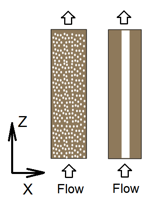
The following gives an example of setting up flow and transport calculations in 2D homogeneous and heterogeneous domains. Here we use the physical set up of 2D cross-sections of the Mixed and One-zone column in (Li et al., 2014). The authors packed 4 columns of 2.5 cm in diameter and 10.0 cm in length with relatively similar amount of magnesite and quartz distributed in different spatial patterns. Here we focus on two columns that represent two extreme cases: the Mixed column with uniform distributed magnesite and quartz, as well as the One-zone column with magnesite all gathered in one cylindrical zone of diameter of 1.0 centimeter. To keep it simple, here we will do the calculation for 2D cross-sections, instead of following the steps in section 3.2.4 in the paper to convert 2D to 3D. So our numbers might be different from the paper. We are also assuming that in the middle one zone magnesite is 100% of the solid phase. The 2D system has a size of 25 mm by 100 mm. A constant differential pressure is imposed at the boundaries in the z (vertical) direction, leading the primary water flow direction in the z direction from the bottom to the top. No flux boundaries are specified in the X direction (Li et al., 2014).
| Columns | Mg zone |
Qtz zone | $^2a_L$ (cm) |
$^4a_T$ (cm) |
$\mathrm{\kappa}_e$ (×10-13m2) |
$\phi_{\mathrm{avg}}$ |
|---|---|---|---|---|---|---|
| Mixed | 0.05 | 0.005 | 8.26 | 0.44 | ||
| One-zone | Width: 1.0 cm
$\Phi_{Mg:}\ 0.54$ |
Width: 1.5 cm $\Phi _{Qtz:}\ 0.38$ |
0.07 | 0.004 | 10.74 | 0.44 |
*The permeability of the pure sand columns of the same grain size was measured to be $8.7 \times 10^{-13} \mathrm{~m}^{2}$.
Please do the following:
- Given the effective permeability of the One-zone column and the pure sand column, calculate the permeability of the magnesite zone based on the arithmetic average of the equation;
- Calculate the volume fraction of the magnesite and quartz assuming the two columns have the same total mass and volume fraction of magnesite and quartz;
- Following descriptions in Li et al. (2014) Fig. 1, calculate the pressure field needed for each column in order to have a flow velocity of 3.6 m/day;
- What is the residence time when the flow velocity is 3.6 m/day?
Run the simulation at the grid block resolution of 1 mm by 1 mm.
- Generate the flow field of the two columns. What is flow velocity in the homogeneous column? What is the flow velocity in the magnesite and sand zone of the One-zone column? What is the ratio of the flow velocity between the two zones? Are they consistent with the permeability ratio of the two zones?
- If we inject Br at the concentration of 1.2×10⁻⁴ mol/L at the inlet, please generate the bromide breakthrough curves for the two columns. Note that here you will assume that you only one outlet that integrate all the flow and concentration coming out the outlet grid blocks using the equation
\begin{equation}C_{a v g}=\sum_{i=1}^{n} C_{i} q_{i} / \sum_{i=1}^{n} q_{i}\end{equation}where Ci and qi are the concentration and flow rate from the grid block i in the outlet cross-section. Please plot the overall breakthrough curves from the two columns and discuss their differences.
Note: in plotting 2D figures, you can use softwares such as Tecplot or Matlab. Penn State provides free Matlab web access on WebLabs at Penn State. You can access matlab from there. In addition, you can also get video tutorials from LinkedInLearning at Penn State about using matlab.
Lesson 8 - Mixed 2D.1 Video (56:05 minutes)
Li Li: All right, so this is the video for lesson eight, continued. We just finished doing the homogeneous column. 2D, we call that-- mixed 2D. So you should have watched that first, before you start this one, because the other one has a lot of backdoor information that I provided.
And on top of that, we made the mistake of missing that keyword, zone, in specified permeability. So hopefully, that helps you remember. This is very important.
And then, you have-- I guess, that's the value of making mistakes from my side. And then, you see how things are fixed, and all that. So here, we are going to-- in this one, I'm going to talk about how to do the one zone case. And again, we'll be specifying all the different keyword blocks starting from specify the domain, and then flow, and then transport, and then the reaction-- and then, the initial condition, boundary condition, and all that. So it will be followed in order.
And first, let's also start with discretization. And again, we're using 25 by 100 grid blocks-- 2,500 grid blocks. So essentially, you would have the same discretization. For example, just like what we did before for the homogeneous case-- distance_units. And you would have millimeters. And then, you have xzones-- 25 and space in 1.0 millimeter. Y zones-- you have 100, again 1.0 millimeter as a space.
And then, you are going to specify your domain. But now, we can not specify porosity directly, because there's average porosity, but there's also porosity in different zones, as they are different. The middle zone it's magnesite. The offsite zone is quartz.
And they have different porosity. So we are now going to specify fixed porosity. So here, we are going to just do a porosity update, whatever it is.
And then, we do need to specify the minerals, because different minerals are your different parts of the column. So you actually need magnesite. You also need quartz. And then, you will be specifying different mineral in different parts of the column.
So let's do flow first, just like what we did before, because you do need to calculate its flow, for the flow units are all-- everything you need to calculate the flow field. So again, we are doing time units being seconds. And then, you have distance units being meters. And then, you have calculate flow, true.
So then, you will be specifying permeability. So when you specify permeability, when you do default, you do need to really specify your zone. So I'm going to specify for everything to be 8.74E-13, which is a permeability of the cross-zone first. So when I do default, that means a whole domain have this permeability.
Why do I do that? Because then, I don't need to specify separately. Later on, we'll override. I will specify the magnesite side part, and then override that. So this is the permeability of-- you can specify for the whole domain default. You don't specify zones.
But then I write, later on, permeability_x for the magnesite zone. We calculate that in that, before they're doing this simulation. It's for the middle zone, right? So you have one centimeter with magnesite zone in the middle, and then 0.75 choosing the two other side there.
So into my grid blocks, you would have 8 to 18. Fluctuation, be 9 to 18, is-- sorry-- is the middle magnesite zone.
You would also have this. 13 points-- so that's for the magnesite. Or this would be y. So that specifies the magnesite zone permeability.
OK, so by doing that-- so first of all, here, I specify everywhere is have this value. Now, later, I specify in these zones, you would have these values. So this part of a zone will be overwritten by these values. And the original ones that is not specified is going to remain the same. So you still have-- quartz zone have this value, but the middle of magnesite is going to be overwritten by these values.
And then again, we're going to specify permeability_x like the no-flow boundaries. And you would have zone 0-0, 26-26, as these other ghost cells from-- I'm sorry, 0-0, 1-100, 1-1. And they are permeability_x, 0. And then, again, this zone is very important-- 26, 26.
Actually, I might made a mistake in the previous [INAUDIBLE]. It should be-- really it's a ghost cell outside of the grid block one for x, grid block 25 for x, because these are the no-flow boundary. Again, this will be no flow. So if I made a mistake, make sure you know that was a mistake-- no-flow boundary.
All right, that's permeability. And then, we need to specify pressure. Now see, again, we put the value upon one everywhere. This doesn't really matter. The code we essentially use Darcy's Law given the heterogeneous distribution of permeability and then discretization. So whatever initial value is going to be erased, but we don't want to leave it undefined.
Pressure in that will be 3890. We do the calculation in that before we do the simulation. But again, specified zone will be in the 1-25 in the ghost cell just before you have grid block one. One fix, and then you have pressure, zero again. Zone 1-25-- that's the x. And then, y is 101-101 fix.
So that's a flow. So you are supposed to have everything you need to calculate the flow field. Then, let's look at transport.
Transport will be very similar to what we had before. We need all these dispersion diffusion-related distance units, again, with the centimeters. Time units-- seconds. And then, I'm going to do the same fix diffusion as what we did in the previous one-- 6.342E-6. And then, you have cementation exponent-- cementation, dispersivity.
Dispersivity-- again, the first one is for x, and the second one is for y. So according to the number in the table, you have 0.004, 0.07 centimeters for the two dispersivities. So that's for the transport. And then we need to specify [INAUDIBLE] of the column. Now in here, you have two different zones. One is quart zone. The other is magnesite zone. So we actually specify the two minerals. First of all, we need to specify the primary species.
Now I talk about before, this is a tracer test. So we definitely would need bromide. But also [INAUDIBLE] you put different minerals, you need all the elements, building blocks for that mineral. So for magnesite, you need Mg2 plus because it's MgCO3, so you also need CO2 aq. You need carbonate species.
For quartz, you would need the aqueous species SiO2 aq. But also it is in water. So let's just put H plus there. Just in case some [INAUDIBLE], for example, magnesite is written in terms of H plus. And then second species, you will need OH minus. These species don't really matter in the tracer test. But it will be important later on. But since we are going to specify different mineral zones, even where only for physical process, we do need all the chemical building blocks.
So CO2 aq, then you need bicarbonate, carbonate species. I believe that's it. So these are primary species. And then you need to specify your inlet. Let's just copy all the primary species then, because we know we need that. Inlet, just like what we had before. Units, let's still do molar. Just to be consistent, let's still do molar.
Temperature, bromide, OK, inlet, you have bromide concentration of 1.210 e minus 4. Magnesium, we consider this clean water. So let's just put very low concentration there. Here we also put very low concentration in SiO2, we have low concentration. Because this doesn't really matter at this point. And maybe we put a pH of 7.0. Shouldn't really matter because it's not going to calculate that much anyway.
So for the condition, in the column we have quartz zone and we have magnesite zone. So essentially, we will need both of these. And then primary species, this would be initial in the quartz part. So let's see, still do low concentration bromide. But here, notice these are specified in the aqueous phase. Now we are also going to specify the solid phase.
And for quartz zone, we talk about the positive quartz zone is 0.38. So that means the solid phase is 0.62. So you would have quartz is essentially volume fraction of 0.62. And you put magnesite because you don't have magnesite there. You are going to put very low value.
So essentially, that will give you-- the code will calculate, OK, you have this much solids with a total solid phase of 0.62, then you will calculate porosity being 0.38. I'm just making notes here.
So for magnesite zone, we will still having the whole thing accept the solid phase is different. Because for magnesite, you still have initial condition, that much of these species. But now your quartz will be very small number.
And then your magnesite, remember your magnesite porosity is 0.54. So your magnesite mole volume fraction should be 0.46. So that adding up to be 1. You have the different conditions, just to avoid confusion. So that's the three conditions-- inlet, quartz, magnesite.
Let's specify for the initial conditions. At first, let's specify the whole domain. So there is more quartz [INAUDIBLE] let's specify the whole domain being quartz. So you're putting like one to 25, and then 1 to 100, [INAUDIBLE] for quartz. So that's saying, everywhere you have quartz.
But then, I'm going to override that, the middle part which is nine to 18 will be the magnesite. We're taking the magnesite initial conditions. So that's it gives you, specify initial condition. Then we need a boundary condition. Where is boundary condition?
For the boundary condition, it will be very similar, x_begin, y_begin, x would be inlet. And then you have flux. x_end. Let's say you will do quartz. It doesn't matter much. It's inlet that it is important. And y_begin, y_end. So again, it will take whatever it is coming out of the column. It shouldn't really matter. Boundary condition.
And then you have output. Again, you need to specify how frequently you want things to-- how long do you want to run, how frequent you want output, where do you want output. Spatial profiles, specify, let's do it the same as what we had before-- 0.0011, 0.1, 0.15, and maybe then 0.2. So run the same time as the previous one.
And let's do the time series output, maybe also for the middle. But if you want to look at every outlet block, you're welcome to do that. You don't have to have only one.
For example, you can specify 25 different time series for all the alternate block. Let's say I'm just doing another one time series. Breakthrough, let's say I'm looking at 20. And then [INAUDIBLE] 20, 100, 1. So now you have two different groups. You're looking at the 13 square blocks in the outlet cross section and then 20 square blocks in the outlet.
And then you will be output since this is tracer test. So all that matters to us is bromide. And then we have times series interval should be whatever, 4, 10, or whatever works. All right.
So that seems all we have. Just kind of quickly looking through. I usually try to be clear about what I put in and what are keywords and not making it too crowded. So I'm going to separate that because a lot of times it's easier to see. Line up boundary condition, transport, porosity, discretization, minerals.
For minerals, it's important that you realize that for the name of the minerals, you need the capital in the first letter. Otherwise, the code doesn't recognize it. And then flow, and then you define all the calculated flow, permitted value, permitted value, make sure I have all the zones there when I define specific zone for certain numbers. Zone, zone, OK.
All right. Primary species, secondary species, initial condition, quartz, magnesite. That's consistent always. Let me see. Initial condition, let me just make sure. Yeah, it's consistent with [? permitted that I ?] set up.
Condition inlet, you're putting high concentration bromide and then condition quartz, condition magnesite. You're putting specific volume fraction quartz in various fraction of magnesite, for them to be adding up to be 1 with porosity. All right. So it looks like all right. Let's try it.
So it looks like it's taking this in. And we didn't make mistake again this time, which is good. So first timestamp, it spit it out. And I want to point you to the velocity. So the reasons there's velocity and velocity evolved is because I'm putting porosity to update. So the code will try to update the porosity, although there's no reaction going on or anything. But that's fine.
And then you have porosity. So let's look at velocity. You will realize the velocity is different for different zones, as you can see. And that's more or less because we have different-- permitting different zone. So for this 2D, you will need either product. So spatial profile in 2D like [? Techprod ?] or Matlab, whatever software you use.
The x velocity is not very meaningful. So I would say you just plot the y velocity, which is in direction of the flow. And you realize, OK, y is 1.07. They all have the same units. You're going to go back and check with the corresponding [INAUDIBLE] But in any case, this is 1.07. This is 1.68. Because we just have two zones. And you could imagine this would be the one in the middle zones. And magnesite has a little bit higher probability.
In any case, if you divide 1.68 to 1.07, you get about 1.6 or something. And you realize that when you put the input file, the permitted value of the magnesite is about 1.6 times of the quartz zone. So essentially, the flow is distributed according to the permitted values.
And if you [INAUDIBLE] it should come up with, for example, flow velocity distribution somewhat like the figure one that are we showed with different flow velocity and everything in different places. It's still calculating. It seems really slow for some reason. It's to the 6.35 times 10 to minus 2. OK, still have a bit of time to go.
Because we have more species. And even though we don't really care about these species, we just have to put them there. And the code will try to calculate everything, I'm sure. So it's slower than the homogeneous column.
But in any case, the breakthrough, so for the velocity-- and actually for even let's look at total concentration. So you have x and y. And then you have all different species. But all your K is bromide. So you will be looking at, there's a third column. When you try to calculate the overall breakthrough, imagine you have the 2D. And then in each of the grid block in outlet, you have, for example, let me just go back. It's probably easier to explain with a figure.
This really should be x and y, not x and z. I will change that. In any case, this is your x direction. And this is your y direction. So the [INAUDIBLE] will come out flow velocity different when y equal to 100. This will be y equal to 1, y equal to 100. And this is x.
So you will have different flow velocity coming out from each of the outlet grid blocks. You will also have different concentration coming out because of different [INAUDIBLE]. So what I'm asking you to do, for example, I'll specify a little bit, the concentration average, imagine when we take sample, we actually only have one outlet, not like everywhere you have a sampling point. So that one outlet is essentially integrating all the concentration and flow velocity out of it. So when you calculate average breakthrough, you actually use a flow rate weighted average to do the calculation.
So it would need to be like CI coming out from each of these times, VI and cross section I of each out of this. That way, you get flow rate times concentration, which is mass per time for integrating summation [INAUDIBLE] grid block and divided by the overall flow rate. That will give you the average breakthrough.
So what you need to do when you look at these would be you look at bromide. And you will be looking at y equal to 100. In the example, you get each value, the flow velocity. Cross section area is area of the grid block times porosity. Velocity times that cross section area times the concentration is what you get for each grid block. And then you add them up, divided by the overall flow rate. So that's what you are going to do when you do the breakthrough curve.
And you are going to see a bit of difference in the mix column and in the 2D column. I'm not going to tell you at this point. But in any case, this is what you are going to do. Now we're at 0.16. So we have a little bit. I think we specified to 0.2. So you still have a little bit of time to go. So that's total concentration.
Let me just leave it open. One more. The permitted will give you the distribution of the permitted in different parts of the grid block. These have the units of log 10 meters squared. So these are in log units.
Porosity, [INAUDIBLE] you have xy. And then you have porosity somewhere. For the magnesite zone, you have 54% porosity. And 38 is 38%. So these are the output files. Let me see. Rate, we're not really interested in that.
So it has velocity. If you do have [INAUDIBLE] dissolving out, it will be updating the porosity, permeability, and everything, according to the porosity-permeability relation in the code. And that actually will give you different distributional porosity and permeability from the initial values over time.
I think we are done. Everything is out. And all you need to do is plot thing out and look at the difference in the breakthrough curve, think about why they are different. And you would do-- be interesting to think about how they are different, why they are different, and all that. And I think this is the one zone example with heterogeneity. And you can specify all that.
There is another option. Let's see if you have kind of random distribution of permeability. We can specify in another separate file and [INAUDIBLE] code to read permeability for like irregularly shaped heterogeneity distribution. And this, we're not going to cover. It's a little bit too complicated for now.
So I'm going to stop here. And I'm sure you will have fun. It'll take a little bit more work. But it's also very interesting and very useful when you think about heterogeneity of system, how physical processes are different.
And later on, there will be another session. In Unit Three, we'll be taking about 2D reactive. So this is really building the physical process for that unit later on for the reactive one. All right. I'm going to stop here. I think this is a bit too long.
Solution
-
Effective permeability of the One-zone column:
$\kappa_{\text {eff-onezone }}=10.74 \times 10^{-13} \mathrm{m}^{2}$Pure sand column permeability:
$\kappa_{\text {sand }}=8.74 \times 10^{-13} \mathrm{m}^{2}$This indicates that the permeability of sand zone in the One-zone column is $8.74 \times 10^{-13} \mathrm{m}^{2}$. As the sand and magnesite zones are layered parallel to the flow direction, we can apply Equation (4) to solve the magnesite zone permeability:
$\kappa_{a}=\frac{1}{n} \sum_{i=1}^{n} \kappa_{i}$Here, the volume fraction for sand zone is:
$\left(D_{\text {column }}-D_{\text {magnesite-zone }}\right) / D_{\text {column }}=(2.5-1.0) \mathrm{cm} / 2.5 \mathrm{~cm}=0.6$The volume fraction for magnesite zone is:
$1-0.6=0.4$Hence,
$\begin{array}{l}\kappa_{\text{eff-onezone }}=0.6\kappa_{\text{sand-zone }}+0.4\kappa_{\text{magnesite-zone }}\\
\kappa_{\text{magnesite-zone }}=\frac{\kappa_{\text{eff-onezone }-0.6\kappa_{\text{sand-zone }}}}{0.4}\\
=\frac{10.74\times10^{-13}-0.6\times8.74\times10^{-13}}{0.4}\mathrm{m}^2\\
=13.74\times10^{-13}\mathrm{m}^2\end{array}$ -
In the One-zone column, the magnesite volume fraction = volume fraction of magnesite zone * $\left(1-f_{\mathrm{Mq}}\right)=0.4^{*}(1-0.54)=0.184$. In the Mixed column, the average porosity is 0.44 so the solid phase volume fraction is 0.56. The Mixed column should have the same total amount of magnesite volume as in One-zone column. Therefore The volume fraction of magneiste in the Mixed column = 0.184 and the volume fraction of quartz is the Mixed column = 0.56 – 0.184 = 0.376.
-
We can apply Darcy's Law, Equation (7) to calculate the pressure gradient:
$\kappa_{e}=\frac{u \mu \Delta L}{\Delta P}$Here,
$\begin{array}{l}
u=3.6 \mathrm{~m} / d a y=4.17 \times 10^{-5} \mathrm{m} / \mathrm{s} \\
\mu=1.002 \times 10^{-3} \mathrm{Pa} \cdot \mathrm{s} \\
\Delta L=10.0 \mathrm{~cm}=0.10 \mathrm{m}
\end{array}$For the Mixed column,
$\kappa_{e f f-m i x}=8.26 \times 10^{-13} \mathrm{m}^{2}$Hence,
$\begin{aligned}\Delta P_{\text{mix }}&=\frac{u\mu\Delta L}{\kappa_{\text{eff-mix }}}\\
&=\frac{4.17\times10^{-5}\times1.002\times10^{-3}\times0.10}{8.26\times10^{-13}}Pa\\
&=5.06\times10^3\mathrm{Pa}\end{aligned}$For the One-zone column,
$\kappa_{\text {eff-onezone }}=10.74 \times 10^{-13} \mathrm{m}^{2}$Hence,
$\begin{aligned}\Delta P_{\text{one-zone }}&=\frac{u\mu\Delta L}{\kappa_{\text{eff-onezone }}}\\
&=\frac{4.17\times10^{-5}\times1.002\times10^{-3}\times0.10}{10.74\times10^{-13}}\mathrm{Pa}\\
&=3.89\times10^3\mathrm{Pa}\end{aligned}$ -
$\tau=\frac{L \phi}{u}=\frac{0.1 \times 0.44}{3.6}=0.0122 d a y$
Insert a video for setting up flow and transport calculation in CrunchFlow here.
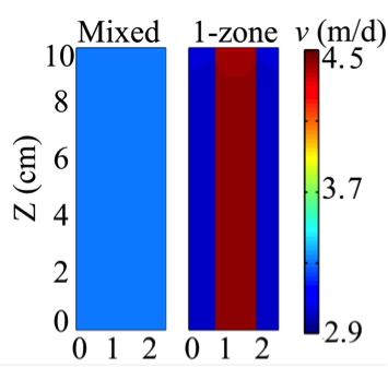 Figure 6: Flow fields of the Mixed and One-zone columns(figure from (Li et al., 2014))
In the homogeneous case, the flow velocity is 3.6 m/day for all the locations. For the One-zone column, the flow velocity in the magnesite zone is 4.5 m/day while the flow velocity in the sand zone is 2.9 m/day. The ratio of flow velocity between the magnesite zone and sand zone is 1.6, which is constant with the permeability ratio of the two zones.
-
For the 2D homogeneous domain, results should be similar to the 1D example in the lesson Flow and Transport Processes in 1D system except there is an additional parameter transverse dispersivity aT, a quantitative measure of dispersion in the direction transverse to the flow. Note that the aT value should not change the shapes of breakthrough curve as a function of residence time in the 2D homogeneous case because there is no transport limitation in the direction transverse to the main flow. Readers can analyze the sensitivity of differential pressure, dispersivity, molecular diffusion coefficient, and cementation factor.
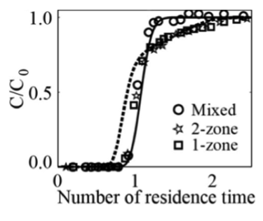 Figure 7. Breakthrough curves of the two columns (figure from (Li et al., 2014)).