Earlier in this lesson, we discussed transmission congestion and Locational Marginal Prices. As you can see in Figure 2. LMPs are highly volatile. They are calculated at thousands of different locations and change almost constantly. You may also notice that the difference between LMPs at various locations is also volatile. Sometimes the price at one node is higher than at another node, and sometimes it is lower.
We generally define two dimensions of risk in electricity markets: temporal risk and locational or "basis" risk.
Temporal Risk
Temporal risk pertains to volatility in the LMP at a specific location over time; Risk associated with variation in a node or zone of prices over time. Temporal risk arises due to changes in electricity demand and fuel prices at a specific location.
Locational or "Basis" Risk
Locational or "basis" risk pertains to volatility in the LMP across space (between two or more locations); Risk associated with variation of the transmission price between two nodes or zones. This is the same thing as variation in the difference between two LMPs or zonal prices. Locational risk is sometimes referred to as “basis risk” in the electricity industry.
These two types of risk may need to be managed through various hedging instruments, but they also may represent arbitrage opportunities.
Two of the most common ways of exercising arbitrage in electricity markets are through "virtual bidding" (arbitraging the difference between the clearing price in the day-ahead and real-time electricity market) and through the "spark spread" (the difference between fuel and electricity prices).
Virtual Bidding
Virtual bidding offers a mechanism for electricity market participants to take advantage of differences between day-ahead and real-time prices at a specific location. It involves buying or selling some quantity of electricity in the day-ahead market, and then taking an offsetting position in the real-time market. Large financial institutions like investment banks and hedge funds engage in a lot of virtual bidding, but other types of market participants like generating companies and electric utilities also engage in virtual bidding. The mechanics of virtual bidding are very simple. A market participant first takes a short or long position in the day-ahead market. A short position is known as a "dec" and a long position is known as an "inc." If that market participant's inc or dec clears the day-ahead market (in other words, if that participant would get dispatched if it represented an actual physical need to buy or sell electricity), then the market participant must take an offsetting position in the real-time market. So, a day-ahead dec would be paired with a real-time inc, and a day-ahead inc would be paired with a real-time dec. The quantities offset one another and in the end, the market participant does not have to buy or sell any actual electricity. But the market participant is paid the LMP for the inc and pays the LMP for the dec.
For example, a market participant submits a 1 MW inc in the day-ahead market, believing that the day-ahead price will be greater than the real-time price. We'll say that the inc clears the market and the day-ahead LMP is $25/MWh. This same market participant would submit a dec to the real-time market, and we'll say that the dec clears the real-time market and the real-time price is $20/MWh. What has basically happened is that this market participant has sold 1 MWh of energy at $25/MWh and bought that same MWh for $20, netting $5 in profit.
Spark Spread
The second mechanism for exercising arbitrage is through the "spark spread," which is the difference between the electricity price and the cost of generating electricity, which is mainly the fuel cost. The arbitrage opportunity that the spark spread represents is typically the opportunity to buy fuel and sell electricity. Spark spreads in financial markets are typically defined as the difference between the LMP and the cost of producing electricity by a natural gas generator with certain characteristics (like a heat rate of 10,000 and variable O&M costs of $2.50 per MWh).
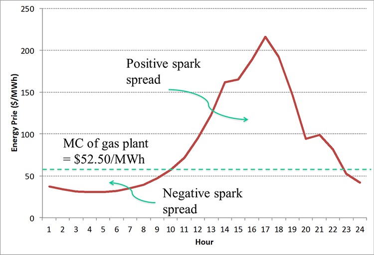
As an example, let's say that the electricity price is $100/MWh and the cost of fuel is $5 per million BTU. The marginal cost of a gas-fired generator at this fuel price with a heat rate of 10 million BTU/MWh and variable O&M costs of $2.50/MWh would be 10*5 + 2.50 = $52.50/MWh. The spark spread would thus be $100/MWh - $52.50/MWh = $47.50/MWh.
The figure below shows some historical LMPs in PJM as compared to our hypothetical gas generation marginal cost of $52.50/MWh. During some hours, the spark spread is negative, indicating that it would not be profitable to buy fuel and sell electricity. During other hours, the spark spread is positive, indicating that it would be profitable to buy fuel and sell electricity.