3.2.1: Step 1 -- Preparing the Data for Estimating the Reserve

3.2.1: Step 1 -- Preparing the Data for Estimating the Reserve

As a starting point, you’re likely to have the following:

• a table of the coordinates of each drill hole,
• the drill log for each hole, and
• analytical results from each hole.

Here are examples of each of these.

The table of coordinates may look like this:

Here is a section for a typical drill log. The complete drill log for this hole can be viewed here: Driller’s Log.pdf, and you should look at the full log.

The analytical results will come from laboratory studies to determine the aforementioned parameters of interest. Here is an example taken from the lab results for the sample obtained from one drill hole.

Figure 3.2.1: Example of analytical results

SGS North America, Inc.

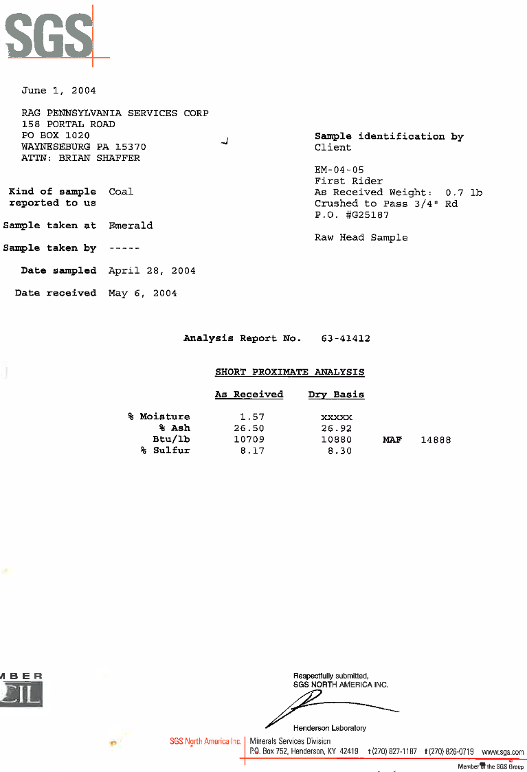
The complete lab report for this hole can be viewed here: Reserve Estimation.pdf

There may be multiple lab reports. The example here focuses on the chemical characteristics of the coal. In many cases, we'll conduct physical tests on the cores to determine geotechnical parameters, e.g. compressive strength, on the ore as well as the rock around the orebody.

We will want to build a database that contains the parameters of interest for each of the holes. If we are interested in determining the average grade, then our table will begin with two columns: drill hole number and the grade for the sample from that hole. Let's suppose that we have a property with 9 holes:

We want the average grade for the deposit. Is the average grade equal to the arithmetic average, which is 3.33%?

Are the holes spaced uniformly on a grid, like this?

Figure 3.2.2:  Boundary and holes

Credit: J. Kohler, © Penn State University, is licensed under CC BY-NC-SA 4.0

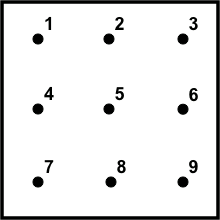
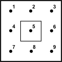
If so, it will be easy to define an area around each hole and then to say that everything within that area has the same properties as those found in the drill hole. Let's draw a box around hole number 5 to illustrate this. Shortly we'll refer to this area as an area of influence.

Figure 3.2.3:  Boundary showing center hole.

Credit: J. Kohler, © Penn State University, is licensed under CC BY-NC-SA 4.0

If the area around each hole were identical, then it would seem reasonable to say that the average grade of this orebody equals the arithmetic average of 3.33%. But wait a minute! We've said nothing about the thickness of the orebody at each hole. Assuming the thickness is identical at each hole, then each hole will represent an identical volume of ore, and computing the arithmetic average yields the correct average grade for the orebody.  

However, it's rare that the orebody thickness would be the same at each hole. For the purposes of this example, let's assume a more realistic case in which the thicknesses vary from hole-to-hole. Logically then, a hole through a thicker section of the orebody will represent a greater volume of ore than a hole through a thinner section. If we simply average the two holes together, we will arrive at an incorrect average grade because we have not accounted for the larger contribution of the one hole into the total. We can correct this by using a weighted average, in which the grade of the hole is increased or decreased to reflect the volume that it represents.