3.2.3: Overview of Reserve Estimation Methods

3.2.3: Overview of Reserve Estimation Methods

The polygon method is an old and established approach based on a simple geometric algorithm, in which we construct a polygon around each hole to determine an area of influence for that hole; and then the total volume directly beneath the polygon is assigned the same values as the drill hole from which we constructed the polygon. We’ll take a closer look at his method shortly.

Another method, known as the triangle method, requires that we connect adjacent holes into triangles. The included area of each triangle is assigned the characteristic not of a single hole, but of the weighted average of the three holes forming the triangle. The weighting of the three holes is based on the length of the drill holes.

The inverse distance method is a more complex scheme in which the contribution of a given hole is weighted according to its distance from the block in which the estimate is to be made. The closer a hole is, the more weight is given to its value compared to the values of other holes in the region.

Geostatistical methods employed for ore reserve estimation utilize three-dimensional spatial statistics to improve the quality of the estimate. Classical statistics requires use of a particular distribution model, e.g., the data are normally distributed, and that the samples be independent of one another. Generally, we have insufficient samples of the orebody to assign a distribution, and moreover, the samples are often correlated, i.e., they do not satisfy the independence requirement of classical statistics. Given that the samples, i.e., the drillholes, are limited in number because they are expensive to acquire, often biased, and nearly always smaller in number than is desired, geostatistics is a powerful tool for improving the quality of the estimation.

A prerequisite to a reasonable prediction of the grade of the orebody is a good prediction of the spatial distribution of the grade, or whatever characteristic is of interest. This spatial estimation is accomplished using the sample data and a model known as a variogram, which is used to represent the correlation between the samples. This estimation is often accomplished using a technique known as kriging. Kriging provides an optimal interpolation using the variogram; and the technique is similar to simple interpolation, as we would use in say the inverse distance algorithm, but is different, because it allows us to take into account information that we know about the geology and attendant properties. Based on geologic knowledge of the presence of a certain feature, we will know that the characteristics of all points contained in that feature should be the same or similar. This is an instance where samples are correlated. With geostatistical methods, we can use this knowledge to improve the estimate of grade, or whatever, at points where we have not sampled. The science of geostatistics continues to evolve, becoming more accurate. You will learn the common geostatistical techniques, their strengths, and limitations in MNG 412.

Today, you can enter your exploration data into a computer program and then within minutes, you can have estimates of the resource from several different methods. Then, you will choose which estimate to use. That choice may be based on experience or a heuristic such as selecting the estimate that has the smallest variance. The commercially available mine planning software programs, such as the Carlson software that we use, allow you to employ several different techniques. We are not going to look into these methods in any greater details in this course, with one exception --the polygon method. This method is useful to illustrate the concepts and is a reasonable estimation method in its own right.

The Polygon Method

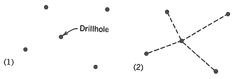
We begin with a map showing the surface location of the drill holes, and our task is to construct polygons around each hole. The relevant characteristic, say grade, inside of that entire polygon will be the same as the value of that characteristic in the drill hole sample.

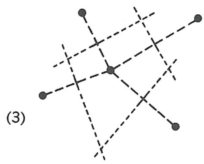
We start our work by arbitrarily selecting a drill hole, and then drawing lines between that hole and all the adjacent holes, as shown here.

Figure 3.2.5: Left (1): drill hole, and Right: (2) lines drawn between the hole and all adjacent holes

From p. 78 of Introductory Mining Engineering, 2nd Ed., Hartman, H.L, and J.M. Mutmansky

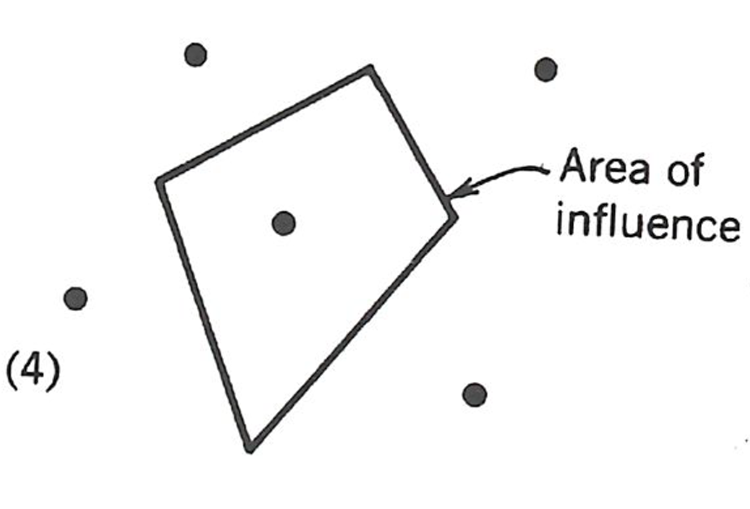
Next, we draw perpendicular bisectors though each of these lines, drawing the bisector line long enough to intersect the other perpendicular bisectors, as shown.

Figure 3.2.6: Bisector lines are long enough to intersect other perpendicular bisectors

From p.78 of Introductory Mining Engineering, 2nd Ed., Hartman, H.L, and J.M. Mutmansky

The corners of the polygon are defined by the intersection of the perpendicular bisectors, as shown.

Figure 3.2.7: Polygon with corners defined by perpendicular bisectors

From p. 78 of Introductory Mining Engineering, 2nd Ed., Hartman, H.L, and J.M. Mutmansky

Watch this video (2:59) of a demonstration of using the Polygon Method.

We repeat the process for each hole. Note that if the hole is adjacent to the property boundary, then that boundary line will form a side of the polygon. The result will be a property containing as many polygons as holes, as illustrated here.

Figure 3.2.8: The result is a property with as many polygons as holes

From p. 78 of Introductory Mining Engineering, 2nd Ed., Hartman, H.L, and J.M. Mutmansky

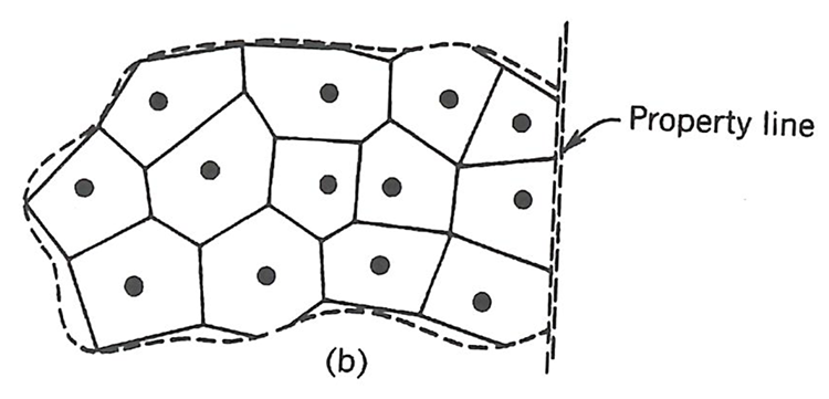
Next, we need to determine the area of each polygon. This can be done manually using a planimeter, or digitally. The result will be an area of influence, i.e., the area of the polygon, for each hole. Then, we can calculate the volume of influence of each polygon, by multiplying the area of influence by the thickness of the ore, or overburden. The next step is to build a table or spreadsheet to facilitate the calculations. We actually did that earlier, in Lesson 3.2.2, and will not repeat it again. At that time, we only calculated the average grade. We could have added any number of other characteristics to the table, and calculated their average value. Examples would include thickness of the deposit and overburden, as well as other characteristics of interest.