OGR and GDAL exist as separate modules in the osgeo package together with some other modules such as OSR for dealing with different projections and some auxiliary modules. As with previous packages you will probably need to install gdal (which encapsulates all of them in its latest release) to access these packages. So typically, a Python project using GDAL would import the needed modules similar to this:
from osgeo import gdal
from osgeo import ogr
from osgeo import osr
Let’s start with taking a closer look at the ogr module for working with vector data. The following code, for instance, illustrates how one would open an existing vector data set, in this case an Esri shapefile. OGR uses so-called drivers to access files in different formats, so the important thing to note is how we first obtain a driver object for ‘ESRI Shapefile’ with GetDriverByName(...) and then use that to open the shapefile with the Open(...) method of the driver object. The shapefile we are using in this example is a file with polygons for all countries in the world (available here) and we will use it again in the lesson’s walkthrough. When you download it, you may still have to adapt the path in the first line of the code below.
shapefile = r'C:\489\L3\TM_WORLD_BORDERS-0.3.shp'
drv =ogr.GetDriverByName('ESRI Shapefile')
dataSet = drv.Open(shapefile)
dataSet now provides access to the data in the shapefile as layers, in this case just a single layer, that can be accessed with the GetLayer(...) method. We then use the resulting layer object to get the definitions of the fields with GetLayerDefn(), loop through the fields with the help of GetFieldCount() and GetFieldDefn(), and then print out the field names with GetName():
layer = dataSet.GetLayer(0)
layerDefinition = layer.GetLayerDefn()
for i in range(layerDefinition.GetFieldCount()):
	print(layerDefinition.GetFieldDefn(i).GetName())
Output:
FIPS
ISO2
ISO3
UN
NAME
...
LAT
If you want to loop through the features in a layer, e.g., to read or modify their attribute values, you can use a simple for-loop and the GetField(...) method of features. It’s important that, if you want to be able to iterate through the features another time, you have to call the ResetReading() method of the layer after the loop. The following loop prints out the values of the ‘NAME’ field for all features:
for feature in layer:
	print(feature.GetField('NAME'))
layer.ResetReading()
Output:
Antigua and Barbuda
Algeria
Azerbaijan
Albania
....
We can extend the previous example to also access the geometry of the feature via the GetGeometryRef() method. Here we use this approach to get the centroid of each country polygon (method Centroid()) and then print it out in readable form with the help of the ExportToWkt() method. The output will be the same list of country names as before but this time, each followed by the coordinates of the respective centroid.
for feature in layer:
    print(feature.GetField('NAME') + '–' + feature.GetGeometryRef().Centroid().ExportToWkt())
layer.ResetReading()
We can also filter vector layers by attribute and spatially. The following example uses SetAttributeFilter(...) to only get features with a population (field ‘POP2005’) larger than one hundred million.
layer.SetAttributeFilter('POP2005 > 100000000')
for feature in layer:
	print(feature.GetField('NAME'))
layer.ResetReading()
Output:
Brazil
China
India
...
We can remove the selection by calling SetAttributeFilter(...) with the empty string:
layer.SetAttributeFilter('')
The following example uses SetSpatialFilter(...) to only get countries overlapping a given polygonal area, in this case an area that covers the southern part of Africa. We first create the polygon via the CreateGeometryFromWkt(...) function that creates geometry objects from Well-Known Text (WKT) strings. Then we apply the filter and use a for-loop again to print the selected features:
wkt = 'POLYGON ( (6.3 -14, 52 -14, 52 -40, 6.3 -40, 6.3 -14))'  # WKT polygon string for a rectangular area
geom = ogr.CreateGeometryFromWkt(wkt)
layer.SetSpatialFilter(geom)
for feature in layer:
	print(feature.GetField('NAME'))
layer.ResetReading()
Output:
Angola
Madagascar
Mozambique
...
Zimbabwe
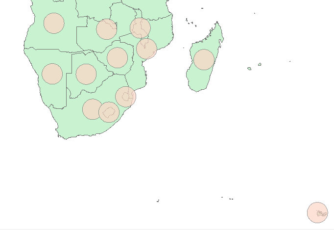
Access to all features and their geometries together with the geometric operations provided by GDAL allows for writing code that realizes geoprocessing operations and other analyses on one or several input files and for creating new output files with the results. To show one example, the following code takes our selection of countries from southern Africa and then creates 2 decimal degree buffers around the centroids of each country. The resulting buffers are written to a new shapefile called centroidbuffers.shp. We add two fields to the newly produced buffered centroids shapefile, one with the name of the country and one with the population, copying over the corresponding field values from the input country file. When you will later have to use GDAL in one of the parts of the lesson's homework assignment, you can use the same order of operations, just with different parameters and input values.
To achieve this task, we first create a spatial reference object for EPSG:4326 that will be needed to create the layer in the new shapefile. Then the shapefile is generated with the shapefile driver object we obtained earlier, and the CreateDataSource(...) method. A new layer inside this shapefile is created via CreateLayer(...) and by providing the spatial reference object as a parameter. We then create the two fields for storing the country names and population numbers with the function FieldDefn(...) and add them to the created layer with the CreateField(...) method using the field objects as parameters. When adding new fields, make sure that the name you provide is not longer than 8 characters or GDAL/OGR will automatically truncate the name. Finally, we need the field definitions of the layer available via GetLayerDefn() to be able to later add new features to the output shapefile. The result is stored in variable featureDefn.
sr = osr.SpatialReference()   # create spatial reference object
sr.ImportFromEPSG(4326)       # set it to EPSG:4326
outfile = drv.CreateDataSource(r'C:\489\L3\centroidbuffers.shp') # create new shapefile
outlayer = outfile.CreateLayer('centroidbuffers', geom_type=ogr.wkbPolygon, srs=sr)  # create new layer in the shapefile

nameField = ogr.FieldDefn('Name', ogr.OFTString)        # create new field of type string called Name to store the country names
outlayer.CreateField(nameField)                         # add this new field to the output layer
popField = ogr.FieldDefn('Population', ogr.OFTInteger) # create new field of type integer called Population to store the population numbers
outlayer.CreateField(popField)                         # add this new field to the output layer

featureDefn = outlayer.GetLayerDefn()  # get field definitions
Now that we have prepared the new output shapefile and layer, we can loop through our selected features in the input layer in variable layer, get the geometry of each feature, produce a new geometry by taking its centroid and then calling the Buffer(...) method, and finally create a new feature from the resulting geometry within our output layer.
for feature in layer:                                              # loop through selected features
    ingeom = feature.GetGeometryRef()                              # get geometry of feature from the input layer
    outgeom = ingeom.Centroid().Buffer(2.0)                        # buffer centroid of ingeom

    outFeature = ogr.Feature(featureDefn)                          # create a new feature
    outFeature.SetGeometry(outgeom)                                # set its geometry to outgeom
    outFeature.SetField('Name', feature.GetField('NAME'))          # set the feature's Name field to the NAME value of the input feature
    outFeature.SetField('Population', feature.GetField('POP2005')) # set the feature's Population field to the POP2005 value of the input feature
    outlayer.CreateFeature(outFeature)                             # finally add the new output feature to outlayer
    outFeature = None

layer.ResetReading()
outfile = None         # close output file
The final line “outfile = None” is needed because otherwise the file would remain open for further writing and we couldn’t inspect it in a different program. If you open the centroidbuffers.shp shapefile and the country borders shapefile in a GIS of your choice, the result should look similar to the image below. If you check out the attribute table, you should see the Name and Populations columns we created populated with values copied over from the input features.
Centroid() and Buffer() are just two examples of the many availabe methods for producing a new geometry in GDAL. In this lesson's homework assignment, you will instead have to use the ogr.CreateGeometryFromWkt(...) function that we used earlier in this section to create a clip polygon from a WKT string representation but, apart from that, the order of operations for creating the output feature will be the same. The GDAL/OGR cookbook contains many Python examples for working with vector data with GDAL, including how to create different kinds of geometries from different input formats, calculating envelopes, lengths and areas of a geometry, and intersecting and combining geometries. We recommend that you take a bit of time to browse through these online examples to get a better idea of what is possible. Then we move on to have a look at raster manipulation with GDAL.