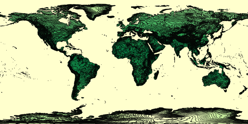
To open an existing raster file in GDAL, you would use the Open(...) function defined in the gdal module. The raster file we will use in the following examples contains world-wide bioclimatic data and will be used again in the lesson’s walkthrough. Download the raster file here.
raster = gdal.Open(r'c:\489\L3\wc2.0_bio_10m_01.tif')
We now have a GDAL raster dataset in variable raster. Raster datasets are organized into bands. The following command shows that our raster only has a single band:
raster.RasterCount
Output:
1
To access one of the bands, we can use the GetRasterBand(...) method of a raster dataset and provide the number of the band as a parameter (counting from 1, not from 0!):
band = raster.GetRasterBand(1) # get first band of the raster
If your raster has multiple bands and you want to perform the same operations for each band, you would typically use a for-loop to go through the bands:
for i in range(1, raster.RasterCount + 1):
    b = raster.GetRasterBand(i)
    print(b.GetMetadata())      # or do something else with b
There are a number of methods to read different properties of a band in addition to GetMetadata() used in the previous example, such as GetNoDataValue(), GetMinimum(), GetMaximum(), andGetScale().
print(band.GetNoDataValue())
print(band.GetMinimum())
print(band.GetMaximum())
print(band.GetScale())
Output:
-1.7e+308
-53.702073097229
33.260635217031
1.0
GDAL provides a number of operations that can be employed to create new files from bands. For instance, the gdal.Polygonize(...) function can be used to create a vector dataset from a raster band by forming polygons from adjacent cells that have the same value. To apply the function, we first create a new vector dataset and layer in it. Then we add a new field ‘DN’ to the layer for storing the raster values for each of the polygons created:
drv = ogr.GetDriverByName('ESRI Shapefile')
outfile = drv.CreateDataSource(r'c:\489\L3\polygonizedRaster.shp')
outlayer = outfile.CreateLayer('polygonized raster', srs = None )
newField = ogr.FieldDefn('DN', ogr.OFTReal)
outlayer.CreateField(newField)
Once the shapefile is prepared, we call Polygonize(...) and provide the band and the output layer as parameters plus a few additional parameters needed:
gdal.Polygonize(band, None, outlayer, 0, [])
outfile = None
With the None for the second parameter we say that we don’t want to provide a mask for the operation. The 0 for the fourth parameter is the index of the field to which the raster values shall be written, so the index of the newly added ‘DN’ field in this case. The last parameter allows for passing additional options to the function but we do not make use of this, so we provide an empty list. The second line "outfile = None" is for closing the new shapefile and making sure that all data has been written to it. The result produced in the new shapefile rasterPolygonized.shp should look similar to the image below when looked at in a GIS and using a classified symbology based on the values in the ‘DN’ field.
Polygonize(...) is an example of a GDAL function that operates on an individual band. GDAL also provides functions for manipulating raster files directly, such as gdal.Translate(...) for converting a raster file into a new raster file. Translate(...) is very powerful with many parameters and can be used to clip, resample, and rescale the raster as well as convert the raster into a different file format. You will see an example of Translate(...) being applied in the lesson’s walkthrough. gdal.Warp(...) is another powerful function that can be used for reprojecting and mosaicking raster files.
While the functions mentioned above and similar functions available in GDAL cover many of the standard manipulation and conversion operations commonly used with raster data, there are cases where one directly wants to work with the values in the raster, e.g. by applying raster algebra operations. The approach to do this with GDAL is to first read the data of a band into a GDAL multi-dimensional array object with the ReadAsArray() method, then manipulate the values in the array, and finally write the new values back to the band with the WriteArray() method.
data = band.ReadAsArray()
data
If you look at the output of this code, you will see that the array in variable data essentially contains the values of the raster cells organized into rows. We can now apply a simple mathematical expression to each of the cells, like this:
data = data * 0.1
data
The meaning of this expression is to create a new array by multiplying each cell value with 0.1. You should notice the change in the output from +308 to +307. The following expression can be used to change all values that are smaller than 0 to 0:
print(data.min())
data [ data < 0 ] = 0
print(data.min())
data.min() in the previous example is used to get the minimum value over all cells and show how this changes to 0 after executing the second line. Similarly to what you saw with pandas data frames in Section 3.8.6, an expression like data < 0 results in a Boolean array with True for only those cells for which the condition <0 is true. Then this Boolean array is used to select only specific cells from the array with data[...] and only these will be changed to 0. Now, to finally write the modified values back to a raster band, we can use the WriteArray(...) method. The following code shows how one can first create a copy of a raster with the same properties as the original raster file and then use the modified data to overwrite the band in this new copy:
drv = gdal.GetDriverByName('GTiff')     # create driver for writing geotiff file
outRaster = drv.CreateCopy(r'c:\489\newRaster.tif', raster , 0 )   # create new copy of inut raster on disk
newBand = outRaster.GetRasterBand(1)                               # get the first (and only) band of the new copy
newBand.WriteArray(data)                                           # write array data to this band
outRaster = None                                                   # write all changes to disk and close file
This approach will not change the original raster file on disk. Instead of writing the updated array to a band of a new file on disk, we can also work with an in-memory copy instead, e.g. to then use this modified band in other GDAL operations such as Polygonize(...) . An example of this approach will be shown in the walkthrough of this lesson. Here is how you would create the in-memory copy combining the driver creation and raster copying into a single line:
tmpRaster = gdal.GetDriverByName('MEM').CreateCopy('', raster, 0) # create in-memory copy
The approach of using raster algebra operations shown above can be used to perform many operations such as reclassification and normalization of a raster. More complex operations like neighborhood/zonal based operators can be implemented by looping through the array and adapting cell values based on the values of adjacent cells. In the lesson’s walkthrough you will get to see an example of how a simple reclassification can be realized using expressions similar to what you saw in this section.
While the GDAL Python package allows for realizing the most common vector and raster operations, it is probably fair to say that it is not the most easy-to-use software API. While the GDAL Python cookbook contains many application examples, it can sometimes take a lot of search on the web to figure out some of the details of how to apply a method or function correctly. Of course, GDAL has the main advantage of being completely free, available for pretty much all main operating systems and programming languages, and not tied to any other GIS or web platform. In contrast, the Esri ArcGIS API for Python discussed in the next section may be more modern, directly developed specifically for Python, and have more to offer in terms of visualization and high-level geoprocessing and analysis functions, but it is tied to Esri’s web platforms and some of the features require an organizational account to be used. These are aspects that need to be considered when making a choice on which API to use for a particular project. In addition, the functionality provided by both APIs only overlaps partially and, as a result, there are also merits in combining the APIs as we will do later on in the lesson’s walkthrough.