We will again use the Spyder IDE and our basic raster code from earlier in the lesson. Spyder has a Profile pane as well which is accessible from the View -> Panes menu. You may need to manually load your code into Profiler using the folder icon. The spyder help for the Profiler is here if you'd like to read it (Profiler — Spyder 5 documentation (spyder-ide.org)) but we explain the important parts below.
Once you load your code, Profiler automatically starts profiling it and displays the message “ Profiling, please wait...“ at the top of the Profiler window. You will need to be a little patient as Spyder runs through all of your code to perform the timing (or alternatively in these raster examples reduce the sample size). You probably remember that we recommended to run multiprocessing code from the command line rather than inside Spyder. However, using the built-in profiler for loading and running multiprocessing code works as long as the worker function is defined in its own module as we did for the vector clipping example to be able to use it as a script tool. If this is not the case, you will receive an error that certain elements in the code cannot be “pickled“ which you might remember from our multiprocessing discussion means those objects cannot be converted to a basic type. We didn't split the multiprocessing version of the raster example into two separate modules, so here we will only look at the non-multiprocessing version and profile that. We won't have this issue when we using other profilers in the following optional sections and in the homework assignment you will work with the vector clipping multiprocessing example which has been set up in a way that allows for profiling with the Spyder profiler.
Once the Profiler has completed you will see a set of results like the ones below.
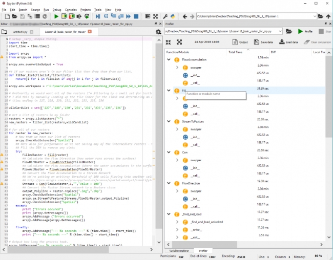
Looking over those results you will see a list of functions together with the times each has taken. The important column to examine is the Local Time column which shows you how long each function has taken to execute in us (microseconds), ms (milliseconds), seconds, minutes etc. The Total Time column is showing you the cumulative time for each of those processes that was run (e.g. if your code was running in a function). You can order any of the columns but if you arrange the Total Time column in ascending order this will give you a logical starting point as the times will be arranged from the shortest to longest running. There is no way to order the results to see the order in which your code ran. So you will see (depending on your code arrangement) overwriteOutput followed by the time function, then filterList, etc.
The next column to look at is the Calls column which has the count of how many times each of those functions was launched. So a high value in Local Time might be indicative of either a large number of calls to a very fast function or a small number of calls to a very slow function.
In my timings, there aren’t any obvious places to look for performance improvements although the code could be fractionally faster (but less of a good team player) if I didn’t check the extension back in and my .replace() method and print add a small amount of time to the execution.
What we are doing with this type of profiling is examining the sum of the functions and methods which were called during the code execution and how long they took, in total, for the number of times that they were called. It is possible to identify inefficiencies with this sort of profiling, particularly in combination with debugging. Am I calling a slow function too often? Can I find a faster function to do the same job (for example some mathematical functions are significantly faster than others and achieve the same result and often there exist approximations that give almost the exact result but are much faster to compute)?
It is worth pointing out here that the results from Spyder’s Profiler are actually the output from the cProfile package of the Python standard library which is essentially wrapped around our script to calculate the statistics we are seeing above. You could import this package into your own code and use it there directly but we will focus on using its functionality from the IDE which is usually more convenient and the results are presented in a more readily understood format.
You might be thinking that these results aren’t really that readily understood and it would be easier if there were a graphical visualization of the timings. Luckily there is and if you want to learn more about it, the following optional sections on code profiling with visualiuation are a good starting point. In addition, we continue another optional section that explains how you can do more detailed profiling looking at each individual line rather than complete functions. However, we recommend that you skip or only skim through these optional sections on your first pass through the lesson materials and come back when you have the time.