As we said at the beginning of this section, this section is provided for interest only. Please feel free to skip over it and you can loop back to it at the end of the lesson if you have free time or after the end of the class. Be warned: installing the required extensions and using them is a little complicated - but this is an advanced class, so don't let this deter you.
Before we begin this optional section, you should know that line profiling is slow – it adds a lot of overhead to our code execution and it should only be done on functions that we know are slow and we’re trying to identify the specifics of why they are slow. Due to that overhead, we cannot rely on the absolute timing reported in line profiling, but we can rely on the relative timings. If a line of code is taking 50% of our execution time and we can reduce that to 40,30 or 20% (or better) of our total execution time then we have been successful.
With that warning about the performance overhead of line profiling, we’re going to install our line profiler (which isn’t the same one that Spyder or ArcGIS Pro would have us install) again using pip (although you are welcome to experiment with those too).
Setting PermissionsBefore we start installing packages we will need to adjust operating system (Windows) permissions on the Python folder of ArcGIS Pro, as we will need the ability to write to some of the folders it contains. This will also help us if we inadvertently attempt to create profile files in the Python folder as the files will be created instead of producing an error that the folder is inaccessible (but we shouldn't create those files there as it will add clutter).
Open up Windows Explorer and navigate to the c:\Program Files\ArcGIS\Pro\bin folder. Select the Python folder and right click on it and select Properties. Select the Security tab, and click the Advanced button. In the new window that opens select Change Permissions, Select the Users group, Uncheck the Include inheritable permissions from this object’s parent box or Disable Inheritance – depending on your version of Windows, and select Add (or Make Explicit) on the dialog that appears.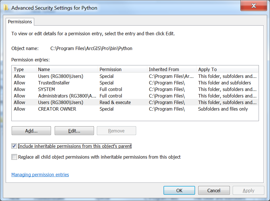
Once again open (if it isn’t already) your Python command prompt and you should be in the folder C:\Program Files\ArcGIS\Pro\bin\Python\envs\arcgispro-py3 or C:\Users\<username>\AppData\Local\ESRI\conda\envs\arcgispro-py3-clone, the default folder of your ArcGIS Pro Python environment, when that command prompt opens (which you can see at the prompt). If in your version of Pro, the command prompt instead shows C:\Users\<username>\AppData\Local\ESRI\conda\envs\arcgispro-py3-clone, then you will have to use this path instead in some of the following commands where the kernprof program is used.
Then type :
scripts\pip install line_profiler
Pip will then download from a repository of hosted Python packages the line_profiler that we need and then install it.
If you receive an error that "Microsoft Visual C++ 14.0 is required," visit https://www.visualstudio.com/downloads/ and download the package for "Visual Studio Community 2017" which will download Visual Studio Installer. Run Visual Studio Installer, and under the "Workloads" tab, you will select two components to install. Under Windows, check the box in the upper right hand corner of "Desktop Development with C++," and, under Web & Cloud, check the box for "Python development." After checking the boxes, click "Install" in the lower right hand corner. After installing those, open the Python command prompt again and enter:
scripts\pip install misaka
If that works, then install the line_profiler with...
scripts\pip install line_profiler
You should see a message saying "Successfully installed line_profiler 2.1.2" although your version number may be higher and that’s okay.
Now that IPython is aware of the line profiler we can run it. There are two modes for running the line profiler, function mode, where we supply a Python file and a function we want to run as well as the parameters for that function given as parameters to the profiler, and module mode, where we supply the module name.
Function-level line profiling is very useful when you want to test just a single function, or if you’re doing multiprocessing as we saw above. Module-level line profiling is a useful first pass to identify those functions that might be slowing things down and it's why we did a similar approach with our higher-level profiling earlier.
Now we can dive into function-level profiling to find the specific lines which might be slowing down our code and then optimize or enhance them and then perform further function-level line profiling (or module-level profiling) again to test our improvements.
We will start with module-level profiling using our single processor Cherry-O code, look at our non-multiprocessing raster example code that did the analysis of the Penn State campus, and finally move on to the multiprocessing Cherry-O code. You may notice a few little deviations in the code that is being used in this section compared to the versions presented in Section 1.5 and 1.6. These deviations are really minimal and have no effect on how the code works and the insights we gain from the profiling.
Our line profiler is in a package called KernProf (named after its author) and it works as a wrapper around the standard cProfile and Line_Profiler tools.
We need to make some changes to our code so that the line profiler knows which functions we wish it to interrogate. The first of those changes is to wrap a function definition around our code (so that we have a function to profile instead of just a single block of code). The second change we need is to use a decorator which is an instruction or meta information for a piece of code that will be ignored by Python. In the case of our profiler, we need to use the decorator @profile to tell KernProf which functions (and we can do many) to examine and it will ignore any without a decorator. Your decorator may give you errors if you're not running your code against the profiler so in that case comment it out.
We’ve made those changes to our original Cherry-O code below so you can see them for yourselves. Check out line 8 for the decorator, line 9 for the function definition (and note how the code is now indented within the function) and line 53 where the function is called. You might also notice that I reduced the number of games back down to 10001 from our very large number earlier. Don’t forget to save your code after you make these changes.
# Simulates 10K game of Hi Ho! Cherry-O
# Setup _very_ simple timing.
import time
start_time = time.time()

import random

@profile
def cherryo():
    spinnerChoices = [-1, -2, -3, -4, 2, 2, 10]
    turns = 0
    totalTurns = 0
    cherriesOnTree = 10
    games = 0

    while games < 10001:
        # Take a turn as long as you have more than 0 cherries
        cherriesOnTree = 10
        turns = 0
        while cherriesOnTree > 0:

            # Spin the spinner
            spinIndex = random.randrange(0, 7)
            spinResult = spinnerChoices[spinIndex]

            # Print the spin result
            #print ("You spun " + str(spinResult) + ".")

            # Add or remove cherries based on the result
            cherriesOnTree += spinResult

            # Make sure the number of cherries is between 0 and 10
            if cherriesOnTree > 10:
                cherriesOnTree = 10
            elif cherriesOnTree < 0:
                cherriesOnTree = 0

            # Print the number of cherries on the tree
            #print ("You have " + str(cherriesOnTree) + " cherries on your tree.")

            turns += 1
        # Print the number of turns it took to win the game
        #print ("It took you " + str(turns) + " turns to win the game.")
        games += 1
        totalTurns += turns

    print ("totalTurns "+str(float(totalTurns)/games))
    #lastline = raw_input(">")

    # Output how long the process took.
    print ("--- %s seconds ---" % (time.time() - start_time))

cherryo()
We could try to run the profiler and the other code from within IPython but that often causes issues such as unfound paths, files, etc., as well as making it difficult to convert our output to a nice readable text file. Instead, we’ll use our Python command prompt and then we’ll run the line profiler using (note: the "-l" is a lowercase L and not the number 1):
python "c:\program files\arcgis\pro\bin\python\envs\arcgispro-py3\lib\site-packages\kernprof.py" -l “c:\users\YourName\CherryO.py”
When the profiling completes (and it will be fast in this simple example), you’ll see our normal code output from our print functions and the summary from the line profiler:
Wrote profile results to CherryO.py.lprof
This tells us the profiler has created an lprof file in our current directory called CherryO.py.lprof (or whatever our input code was called).
The profile files will be saved wherever your Python command prompt path is pointing. Unless you've changed the directory, the Python command prompt will most likely be pointing to C:\Program Files\ArcGIS\Pro\Bin\Python\envs\arcgispro-py3, and the files will be saved in that folder.
The profile files are binary files that will be impossible for us to read without some help from another tool. So to rectify that we’ll run that .lprof file through the line_profiler (which seems a little confusing because you would think we just created that file with the line_profiler and we did, but the line_profiler can also read the files it created) and then pipe (redirect) the output to a text file which we’ll put back in our code directory so we can find it more easily.
To achieve this, we run the following command in our Python command window:
..\python –m line_profiler CherryO.py.lprof > "c:\users\YourName\CherryO.profile.txt"
This command will instruct Python to run the line_profiler (which is some Python code itself) to process the .lprof file we created. The > will redirect the output to a text file at the provided path instead of displaying the output to the screen.
We can then open the resulting output file which should be back in our code folder from within Spyder and read the results. I’ve included my output for reference below and they are also in the CherryO.Profile pdf.
Timer unit: 4.27655e-07 s

Total time: 3.02697 s
File: c:\users\YourName\Lesson 1\CherryO.py
Function: cherryo at line 8

Line #      Hits         Time  Per Hit   % Time  Line Contents
==============================================================
     8                                           @profile
     9                                           def cherryo():
    10         1          5.0      5.0      0.0      spinnerChoices = [-1, -2, -3, -4, 2, 2, 10]
    11         1          2.0      2.0      0.0      turns = 0
    12         1          1.0      1.0      0.0      totalTurns = 0
    13         1          1.0      1.0      0.0      cherriesOnTree = 10
    14         1          1.0      1.0      0.0      games = 0
    15
    16     10002      36775.0      3.7      0.5      while games < 10001:
    17                                                   # Take a turn as long as you have more than 0 cherries
    18     10001      25568.0      2.6      0.4          cherriesOnTree = 10
    19     10001      27091.0      2.7      0.4          turns = 0
    20    168060     464529.0      2.8      6.6          while cherriesOnTree > 0:
    21
    22                                                       # Spin the spinner
    23    158059    4153276.0     26.3     58.7              spinIndex = random.randrange(0, 7)
    24    158059     487698.0      3.1      6.9              spinResult = spinnerChoices[spinIndex]
    25
    26                                                       # Print the spin result
    27                                                       #print "You spun " + str(spinResult) + "."
    28
    29                                                       # Add or remove cherries based on the result
    30    158059     460642.0      2.9      6.5              cherriesOnTree += spinResult
    31
    32                                                       # Make sure the number of cherries is between 0 and 10
    33    158059     458508.0      2.9      6.5              if cherriesOnTree > 10:
    34     42049     112815.0      2.7      1.6                  cherriesOnTree = 10
    35    116010     325651.0      2.8      4.6              elif cherriesOnTree < 0:
    36      5566      14506.0      2.6      0.2                  cherriesOnTree = 0
    37
    38                                                       # Print the number of cherries on the tree
    39                                                       #print "You have " + str(cherriesOnTree) + " cherries on your tree."
    40
    41    158059     445969.0      2.8      6.3              turns += 1
    42                                                   # Print the number of turns it took to win the game
    43                                                   #print "It took you " + str(turns) + " turns to win the game."
    44     10001      29417.0      2.9      0.4          games += 1
    45     10001      31447.0      3.1      0.4          totalTurns += turns
    46
    47         1        443.0    443.0      0.0      print ("totalTurns "+str(float(totalTurns)/games))
    48                                               #lastline = raw_input(">")
    49
    50                                               # Output how long the process took.
    51         1       3723.0   3723.0      0.1      print ("--- %s seconds ---" % (time.time() - start_time))
What we can see here are the individual times to run each line of code: The numbers on the left are the code line numbers, the number of times each line was run (Hits), the time each line took in total (Hits * Time Per Hit), the time per hit, the percentage of time those lines took and, for reference, the line of code alongside.
The first thing that jumps out at me is that the random number selection (line 23) takes the longest time and is called the most – if we can speed this up somehow we can improve our performance.
Let’s move onto the other examples of our code to see some more profiling results.
First we’ll look at the sequential version of our raster processing code before coming back to look at the multiprocessing examples as they’re a little special.
As before with the Cherry-O example we’ll need to wrap our code into a function and use the @profile decorator (and of course call the function). Attempt to make these changes on your own and if you get stuck you can find my code sample here if you want to check your work against mine.
We’ll run the profiler again, produce our output file and then convert it to text and review the results using:
python "c:\program files\arcgis\pro\bin\python\envs\arcgispro-py3\lib\site-packages\kernprof.py" -l "c:\users\YourName\Lesson1B_basic_raster_for_mp.py"
and then
..\python –m line_profiler Lesson1B_basic_raster_for_mp.py.lprof > "c:\users\YourName\Lesson1B_basic_raster_for_mp.py_profile.txt"
If we investigate these outputs (my outputs are here) we can see that the Flow Accumulation calculation is again the slowest, just as we saw when we were doing the module-level calculations. In this case, because we’re predominantly using arcpy functions, we’re not seeing as much granularity or resolution in the results. That is, we don’t know why Flow Accumulation(...) is so slow but I’m sure you can see that in some other circumstances, you could identify multiple arcpy functions which could achieve the same result – and choose the most efficient.
Next, we’ll look at the multiprocessing example of the Cherry-O example to see how we can implement line profiling into our multiprocessing code. As we noted earlier, multiprocessing and profiling are a little special as there is a lot going on behind the scenes and we need to very carefully select what functions and lines we’re profiling as some things cannot be pickled.
Therefore what we need to do is use the line profiler in its API mode. That means instead of using the line profiling outside of our code, we need to embed it in our code and put it in a function between our map and the function we’re calling. This will give us output for each process that we launch. Now if we do this for the Cherry-O example we’re going to get 10,000 files – but thankfully they are small so we’ll work through that as an example.
The point to reiterate before we do that is the Cherry-O code runs in seconds (at most) – once we make these line profiling changes the code will take a few minutes to run.
We’ll start with the easy steps and work our way up to the more complicated ones:
import line_profiler
Now let’s define a function within our code to sit between the map function and the called function (cherryO in my version).
We’ll break down what is happening in this function shortly and that will also help to explain how it fits into our workflow. This new function will be called from our mp_handler() function instead of our original call to cherryO and this new function will then call cherryO.
Our new mp_handler function looks like:
def mp_handler():

    myPool = multiprocessing.Pool(multiprocessing.cpu_count())
    ## The Map function part of the MapReduce is on the right of the = and the Reduce part on the left where we are aggregating the results to a list.
    turns = myPool.map(worker,range(numGames))
    # Uncomment this line to print out the list of total turns (but note this will slow down your code's execution
    #print(turns)
    # Use the statistics library function mean() to calculate the mean of turns
    print(mean(turns))
Note that our call to myPool.map now has worker(...) not cherryO(...) as the function being spawned multiple times. Now let's look at this intermediate function that will contain the line profiler as well as our call to cherryO(...).
def worker(game):
    profiler=line_profiler.LineProfiler(cherryO)
    call = 'cherryO('+str(game)+')'
    turns = profiler.run(call)
    profiler.dump_stats('profile_'+str(game)+'.lprof')
    return(turns)
The first line of our new function is setting up the line profiler and instructing it to track the cherryO(...) function.
As before, we pass the variable game to the worker(...) function and then pass it through to cherryO(...) so it can still perform as before. It’s also important that, when we call cherryO(...), we record the value it returns into a variable turns – so we can return that to the calling function so our calculations work as before. You will notice we’re not just calling cherryO(...) and passing it the variable though – we need to pass the variable a little differently as the profiler can only support certain picklable objects. The most straightforward way to achieve that is to encode our function call into a string (call) and then have the profiler run that call. If we don’t do this the profiler will run but no results will be returned.
Just before we send that value back we use the profiler’s function dump_stats to write out the profile results for the single game to an output file.
Don’t forget to save your code after you make these changes. Now we can run through a slightly different (but still familiar) process to profile and export our results, just with different file names. To run this code we’ll use the Python command prompt:
python c:\users\YourName\CherryO_mp.py
Notice how much longer the code now takes to run – this is another reason to wrap the line profiling in its own function. That means that we don’t need to leave it in production code; we can just change the function calls back and leave the line profiling code in place in case we want to test it again.
It's also possible you'll receive several error messages when the code runs, but the lprof files are still created.
Once our code completes, you will notice we have those 10,000 lprof files (which is overkill as they are probably all largely the same). Examine a few of the files if you like by converting them to text files and viewing them in your favorite text editor or Spyder using the following in the Python command prompt:
python –m line_profiler profile_1.lprof > c:\users\YourName\profile_1.txt
If you examine one of those files, you’ll see results similar to:
Timer unit: 4.27655e-07 s

Total time: 0.00028995 s
File: c:\users\obrien\Dropbox\Teaching_PSU\Geog489_SU_1_18\Lesson 1\CherryO_MP.py
Function: cherryO at line 25

Line #      Hits         Time  Per Hit   % Time  Line Contents
==============================================================
    25                                           def cherryO(game):
    26         1         11.0     11.0      1.6      spinnerChoices = [-1, -2, -3, -4, 2, 2, 10]
    27         1          9.0      9.0      1.3      turns = 0
    28         1          8.0      8.0      1.2      totalTurns = 0
    29         1          8.0      8.0      1.2      cherriesOnTree = 10
    30         1          9.0      9.0      1.3      games = 0
    31
    32                                               # Take a turn as long as you have more than 0 cherries
    33         1          9.0      9.0      1.3      cherriesOnTree = 10
    34         1          9.0      9.0      1.3      turns = 0
    35        16         41.0      2.6      6.0      while cherriesOnTree > 0:
    36
    37                                                   # Spin the spinner
    38        15        402.0     26.8     59.3          spinIndex = random.randrange(0, 7)
    39        15         38.0      2.5      5.6          spinResult = spinnerChoices[spinIndex]
    40
    41                                                   # Print the spin result
    42                                                   #print "You spun " + str(spinResult) + "."
    43
    44                                                   # Add or remove cherries based on the result
    45        15         34.0      2.3      5.0          cherriesOnTree += spinResult
    46
    47                                                   # Make sure the number of cherries is between 0 and 10
    48        15         35.0      2.3      5.2          if cherriesOnTree > 10:
    49         4          8.0      2.0      1.2              cherriesOnTree = 10
    50        11         24.0      2.2      3.5          elif cherriesOnTree < 0:
    51                                                       cherriesOnTree = 0
    52
    53                                                   # Print the number of cherries on the tree
    54                                                   #print "You have " + str(cherriesOnTree) + " cherries on your tree."
    55
    56        15         32.0      2.1      4.7          turns += 1
    57                                               # Print the number of turns it took to win the game
    58         1          1.0      1.0      0.1      return(turns)
Arguably we’re not learning anything that we didn’t know from the sequential version of the code – we can still see the randrange() function is the slowest or most time consuming (by percentage) – however, if we didn’t have the sequential version and wanted to profile our multiprocessing code this would be a very important skill.
The same steps to modify our code above would be implemented if we were performing this line profiling on arcpy (or any other) multiprocessing code. The same type of intermediate function would be required, we would need to pass and return parameters (if necessary) and also reformat the function call so that it was picklable. The output from the line profiler is delivered in a different format to the module-level profiling we were doing before and, therefore, isn’t suitable for loading into QCacheGrind. I'd suggest that isn't as important as we're looking at a much smaller number of lines of code, so the graphical representation isn't as important.
Returning to our ongoing discussion about the less than anticipated performance improvement between our sequential and multiprocessing Cherry-O code, what we can infer by comparing the line profile output of the sequential version of our code and the multiprocessing version is that pretty much all of the steps take the same proportion of time. So if we're doing nearly everything in about the same proportions, but 4 times as many of them (using our 4 processor PC example) then why isn't the performance improvement around 4x faster? We'd expect that setting up the multiprocessing environment might be a little bit of an overhead so maybe we'd be happy with 3.8x or so.
That isn't the case though so I did a little bit of experimenting with calculating how much time it takes to pickle those simple integers. I modified the mp_handler function in my multiprocessor code so that instead of doing actual work selecting cherries, it pickled the 1 million integers that would represent the game number. That function looked like this (nothing else changed in the code):
import pickle
def mp_handler():
    myPool = multiprocessing.Pool(multiprocessing.cpu_count())
    ## The Map function part of the MapReduce is on the right of the = and the Reduce part on the left where we are aggregating the results to a list.
    #turns = myPool.map(worker,range(numGames))
    #turns = myPool.map(cherryO,range(numGames))
    t_start=time.time()
    for i in range(0,numGames):
        pickle_data = pickle.dumps(range(numGames))
    print ("cPickle data took",time.time()-t_start)
    t_start=time.time()
    pickle.loads(pickle_data)
    print ("cPickle data took",time.time()-t_start)
What I learned from this experimentation was that the pickling took around 4 seconds - or about 1/4 of the time my code took to play 1M Cherry-O games in multiprocessing mode - 16 seconds (it was 47 seconds for the sequential version).
A simplistic analysis suggests that the pickling comprises about 25% of my execution time (and your results might vary). If I subtract the time taken for the pickling, my code would have run in 12 seconds and then 47s ÷ 12s = 3.916 - or the nearly the 4x improvement we would have anticipated. So the takeaway message here is the reinforcing of some of the implications of implementing multiprocessing that we discussed earlier: there is an overhead to multiprocessing and lots of small calculations as in this case aren't the best application for it because we lose some of that performance benefit due to that implementation overhead. Still, an almost tripling of performance (47s / 16s) is worth the effort.
Your coding assessment for this lesson will have you modify some code (as mentioned earlier) and profile some multiprocessing analysis code which is why we’re not demonstrating it specifically here. See the lesson assignment page for full details.