This section is provided for interest only. Please feel free to skip over it and you can loop back to it at the end of the lesson if you have free time or after the end of the class.
Creating profile files
Now that we have the QCacheGrind viewer and converter installed we can create some profile files and we'll do that using IPython (available on another tab in Spyder). Think of IPython a little like the interactive Python window in ArcGIS with a few more bells and whistles. We’ll use IPython very shortly for line-by-line profiling, so as a bridge to that task, let's use it to perform some more simple profiling.
Open the IPython pane in Spyder and then you will probably need to change to the folder where your code is located. This should be as easy as looking at the top of the Spyder window, selecting and copying the folder name where your code is, then clicking in the IPython window and typing cd and pasting in the folder name and hitting enter (as seen below).
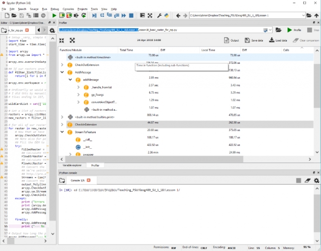
This might look like:
cd c:\Users\YourName\Documents\GEOG489\Lesson1\
We could (but won't) run our code from IPython by typing:
run Lesson1B_basic_raster_for_mp.py
and hitting enter and our code will run and display its output in the IPython window.
That is somewhat useful, but more useful is the ability to use additional packages within IPython for more detailed profiling. Let’s create a function-level profile file using IPython for that raster code and then we’ll run it through the converter and then visualize it in QCacheGrind.
To create that function-level profile we’ll use the built-in profiler prun.
We’ll access it using is a magic word instruction to Spyder which is shorthand for loading an external package; that package is called line_profiler which we just installed. Think of it in the same way as import for Python code – we’re now going to be able to access functionality embedded within that package.
Our magic words have % in front of them. Let's use it to see what the parameters are for using prun with (the ? on the end tells prun to show us its built-in help):
%prun?
If you scroll back up through the IPython console, you will be able to see all of the options for prun. You can compare our command below to that list to break down the various options and experiment with others if you wish. Notice the very last line of the help which states:
If you want to run complete programs under the profiler's control, use "%run -p [prof_opts] filename.py [args to program]" where prof_opts contains profiler specific options as described here.
That is what we’re going to do – use run with the prun options.
cd "C:\Users\YourName"

%run -p -T profile_run.txt -D profile_run.prof
Lesson1B_basic_raster_for_mp
There are a couple of important things to note in these commands. The first is the double quotes around the full path name in the cd command – these are important: just in case there is a space in your path, the double quotes encapsulate it so your folder is found correctly. The other thing is the casing of the various parameters (remember Python is case-sensitive and so are a lot of the built-in tools).
It could take a little while to complete our profiling as our code will run through from start to end. We can check that our code is running by opening the Windows Task Manager and watching the CPU usage which is probably at 100% on one of our cores.
While our code is running we’ll see the normal output with the timing print functions we had implemented earlier. When the run command completes we’ll see a few lines of output that look like :
%run -p -T profile_run.txt -D profile_run.prof
Lesson1B_basic_raster_for_mp

*** Profile stats marshalled to file 'profile_run.prof'.

*** Profile printout saved to text file 'profile_run.txt'.
         3 function calls in 0.000 seconds

   Ordered by: internal time

   ncalls  tottime  percall  cumtime  percall
filename:lineno(function)

        1    0.000    0.000    0.000    0.000 {built-in method
builtins.exec}
        1    0.000    0.000    0.000    0.000
...
        1    0.000    0.000    0.000    0.000
SSL.py:677(Session)
        1    0.000    0.000    0.000    0.000
cookiejar.py:1753(LoadError)
        1    0.000    0.000    0.000    0.000
socks.py:127(ProxyConnectionError)
        1    0.000    0.000    0.000    0.000
_conditional.py:177(cryptography_has_mem_functions)
        1    0.000    0.000    0.000    0.000
_conditional.py:196(cryptography_has_x509_store_ctx_get_issuer)
        1    0.000    0.000    0.000    0.000
_conditional.py:210(cryptography_has_evp_pkey_get_set_tls_enco
dedpoint)
These summary outputs will also be written to a text file that we can open in a text editor (or in Spyder) and our profile file which we will convert and open in QCacheGrind. Writing that output to a text file is useful because there is too much of it to fit within IPython’s window buffer, and you won’t be able to get back to the output right at the start of the execution. If you open the profile_run.txt file in Spyder you’ll see the full output.
Convert output profile files with pyprof2calltree
We’ll run the converter using some familiar Python commands and the convert function within the IPython window:
from pyprof2calltree import convert, visualize
convert('profile_run.prof','callgrind.profile_run')
Open the converted files in QCacheGrind and inspect graphs
The converted output file can now be opened in QCacheGrind. Open QCacheGrind from the folder you installed it into earlier by double-clicking its icon. Click the folder icon in the top left of QCacheGrind or choose File ->Open from the menu and open the callgrind.profile_run file we just created, which should be in the same folder as your source code.
What we have now is a complicated and detailed interface and visualization of every function that our code called but in a more graphically friendly format than the original text file. We can sort by time, number of times a function was called, the function name and the location of that code (our own, within the arcpy library or another library) in the left-hand pane of the interface.
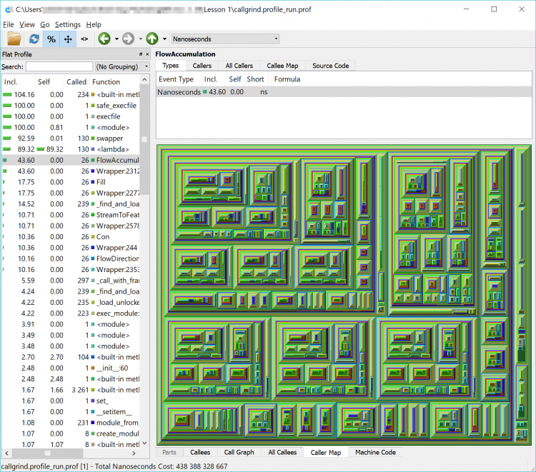
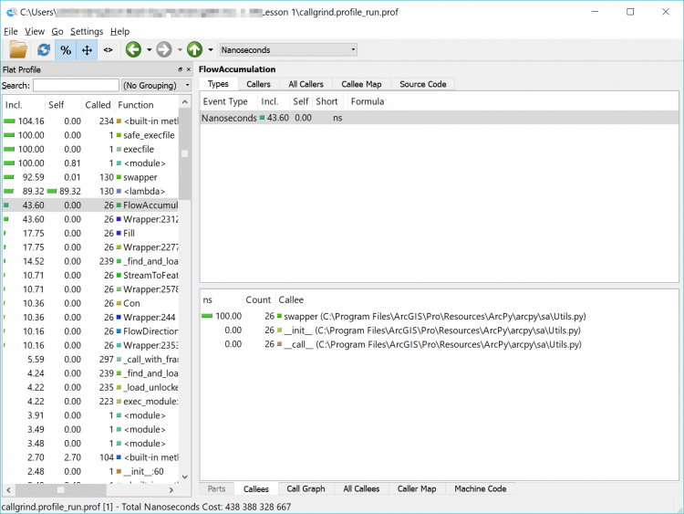
In the list, you will see a lot of built-in functions (things that Python does behind the scenes or that arcpy has it do – calculations, string functions etc.) but you will also see the names of some of the arcpy functions that we used such as FlowAccumulation(...) or StreamToFeature(...). If you double-click on one of them and click on the Call Graph tab in the lower pane you will see a graphical representation of where the tasks were called from. If you double-click on the function’s box above it in the Call Graph pane
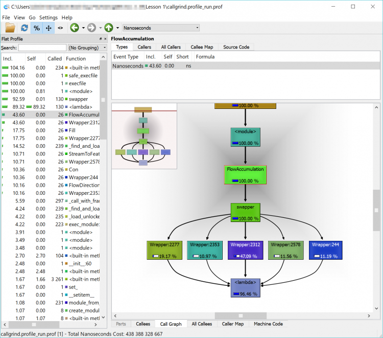
In the example below, we can see that FlowAccumulation(...) is the slowest of our tasks taking about 43% of the execution time. If we can find a way to speed up (or eliminate this process), we’ll make our code more efficient. If we can’t – that’s ok too – we’ll just have to accept that our code takes a certain amount of time to run.
Spend a little time clicking around in the interface and exploring your code – don’t worry too much about going down the rabbit hole of optimizing your code – just explore. Check out functions whose name you recognize such as those raster ones, or ListRasters(). Experiment with examining the content of the different tabs and seeing which modules call which functions (Callers, All Callers and Callee Map). Click down deep into one of the modules and watch the Callee Map change to show each small task being undertaken. If you get too far down the rabbit hole you can use the up arrow near the menu bar to find your way back to the top level modules.
If you’re interested, feel free to run through the process again with your multiprocessing code and see the differences. As a quick reminder, the IPython commands are (although your filenames might be different and be sure to double-check that you're in the correct folder if you get file not found errors):
%run -p -T profile_run_mp.txt -D profile_run_mp.prof Lesson1B_basic_raster_using_mp

from pyprof2calltree import convert, visualize
convert('profile_run_mp.prof','callgrind.profile_run_mp')
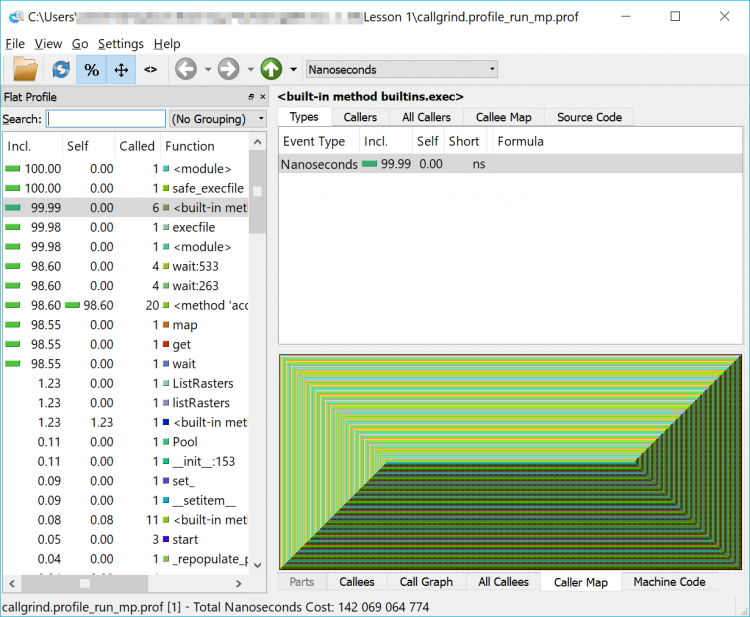
If you load that newly created file into QCacheGrind, you’ll note it looks a little different – like an Escher drawing or a geometric pattern. That is the representation of the multiprocessing functions being run. Feel free to explore among here as well – and you will notice that the functions we previously saw are harder to find – or invisible.
I haven't forgotten about my promise from earlier in the lesson to review the reasons why the Cherry-O code is only about 2-3x faster in multiprocessing mode than the 4x that we would have hoped.
Feel free to run both versions of your Cherry-O code against the profiler and you'll notice that most of the time is taken up by some code described as {method 'acquire' of '_thread.lock' objects} which is called a small number of times. This doesn't give us a lot of information but does hint that perhaps the slower performance is related to something to do with handling multiprocessing objects.
Remember back to our brief discussion about pickling objects which was required for multiprocessing?
It's the culprit, and the following optional section on line profiling will take a closer look at this issue. However, as we said before, line profiling adds quite a bit of complexity, so feel free to skip this section entirely or get back to it after you have worked through the rest of the lesson.