This walkthrough will first give you some experience using the GUI environment of QGIS to clip and project some vector data. Then, you'll learn how to do the same thing using the OGR command line utilities. The advantage of the command line utility is that you can easily run it in a loop to process an entire folder of data.
This project introduces some data for Philadelphia, Pennsylvania that we're going to use throughout the next few lessons. Most of these are simple basemap layers that I downloaded and extracted from OpenStreetMap; however, the city boundary is an official file from the City of Philadelphia that I downloaded from PASDA.
Download the Lesson 3 vector data
Clipping and projecting data with QGIS
- Extract the dataset to a simple path such as C:\data\PhiladelphiaBaseLayers.
- Open the folder and explore it a bit. You'll see a bunch of shapefiles that you can add to QGIS and examine. Also, notice that I have created three folders in preparation for our exercise: clipFeature, clipped, and clippedAndProjected.
- These datasets use a geographic coordinate system and cover the large region of greater Philadelphia. Our processing task is to clip them to the Philadelphia city boundary, then project them into the modified Mercator coordinate system used by popular online web maps (like Google, Bing, Esri, and so forth).
- First, we'll clip and project a dataset using QGIS. This is an easy way to process a single dataset, especially if you're using a tool for the first time.
- Launch QGIS and add fuel.shp and clipFeature/city_limits.shp to the map.
- Click Vector > Geoprocessing Tools > Clip.
- Set the Input vector layer as fuel and the Clip layer as city_limits. Set the output shapefile to be saved in the subfolder as clipped/fuel.shp as shown below. You need to click the ... button, then choose Save to File... and select .SHP for the output format.
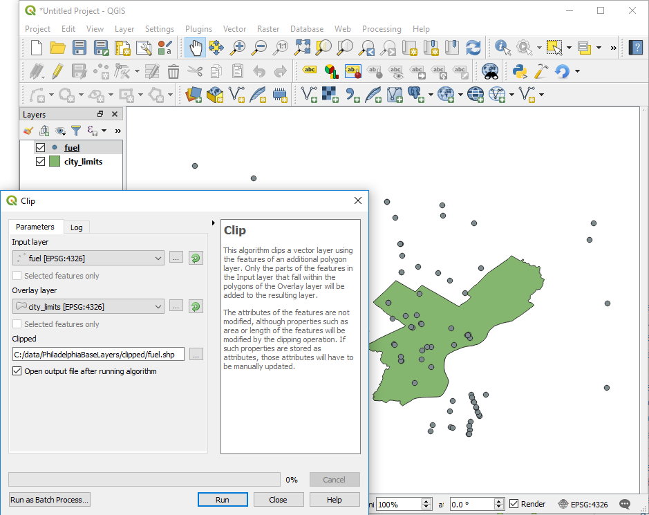 Figure 3.5 Clip tool GUI
 - Select the checkbox for adding the result to the canvas ("Open output file after running algorithm") so you can verify your work. Then click Run. The new layer should only contain features within the boundary of Philadelphia.
Now, let's project this dataset. In QGIS, you do this by saving out a new layer.
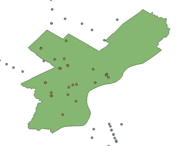 Figure 3.6 Clip tool results
 - In the table of contents, right-click the clipped fuel dataset (not the original one!) and click Export -> Save Features As.... Make sure that the Format box is set to ESRI Shapefile.
- Next to the File name box where you are prompted to put a path, click the ... button and set the path for the output dataset as clippedAndProjected/fuel.shp.
- Next to the CRS box, click the Select CRS button on the right. This is where you'll specify the output projection. The nice thing is that you can search.
- In the Filter box, type pseudo and select WGS 84 / Pseudo Mercator (EPSG: 3857) (not EPSG: 6871). Then click OK.
This projection has lots of names, and we'll cover more of its history in other lessons. For now, remember that you can recognize it using its EPSG code which should be 3857. (Most projections have EPSG codes to overcome naming conflicts and confusion).
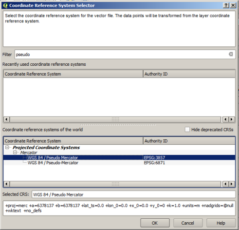 Figure 3.7 QGIS Coordinate reference system dialog
 - Click OK to save out the projected layer. A good way to verify it worked is to start a new map project and add it.
- Create a new map project in QGIS (there's no need to save the old one) and add the clippedAndProjected/fuel.shp file. The layout of the features should look something like what you see below. (I put an SVG marker symbol on this as in Lesson 1, just for fun.)
In QGIS, just like in ArcMap, the first layer you add to the map determines the projection. Notice how the EPSG code in the lower right corner is 3857, proving that my data was indeed projected. If you add any of our other layers to this map, make sure you add them after you add the fuel layer for this reason.
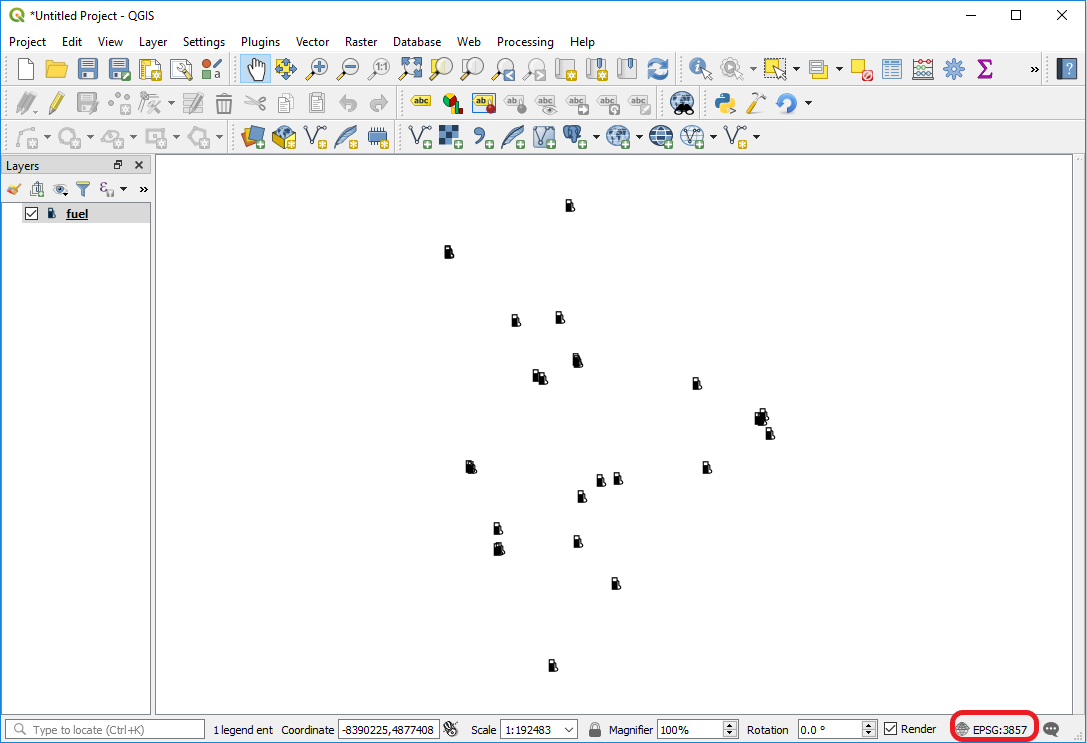 Figure 3.8 Sample QGIS layout showing updated map projection
Clipping and projecting data using the OGR command line utilities
That was easy enough, but it would be tedious, time-consuming, and possibly error prone if you had to do it for more than a few datasets at a time. Let's see how you could use the OGR command line utilities to do this in an automated fashion. Remember that OGR is the subset of the GDAL library that is concerned with vector data.
When you install QGIS, you also get some executable programs that can run GDAL and OGR functions from the command line. The easiest way to get started with these is to use the OSGeo4W shortcut that appeared on your desktop after you installed QGIS.
- Double-click the OSGeo4W shortcut on your desktop. If there's no shortcut, try Start > All Programs > QGIS > OSGeo4W Shell or simply search for OSGeo4W.
You should just see a black command window, possibly displaying some progress output from setting up GDAL and OGR.
We'll walk through the commands for processing one dataset first, then we'll look at how to loop through all files in a folder. For both of these tasks, we'll be using a utility called ogr2ogr. This utility processes an input vector dataset and gives you back a new output dataset (hence, the name). You will use it for both clipping and projecting.
OGR actually lets you do a clip and project in a single command, but, according to the documentation, the projection occurs first. For the sake of simplicity and performance, let's do the clip and the projection as separate actions. We'll do the clip first so we don't project unnecessary data. - Take a look at the documentation for OGR2OGR and see if you can decipher how it's used. When you run this utility, you first supply some optional parameters, then you supply some required parameters. The first required parameter is the name of the output dataset. The second required parameter is the name of the input dataset. These are pretty basic required parameters, so a lot of the trick to using ogr2ogr is to set the optional parameters correctly depending on what you want to do.
- Type the following command in your OSGeo4W window, making sure you replace the paths with your own. Note that this is a single command line with the different parts separated by spaces, NOT multiple lines separated by linebreaks! Also, in case any folder names you use contain spaces, you will have to put the entire paths into double quotes (e.g. "c:\my data folder\PhiladelphiaBaseLayers\...\city_limits.shp").
ogr2ogr -skipfailures -clipsrc c:\data\PhiladelphiaBaseLayers\clipFeature\city_limits.shp c:\data\PhiladelphiaBaseLayers\clipped\roads.shp c:\data\PhiladelphiaBaseLayers\roads.shp
- Wait a few minutes for the command to run. You'll know it's done because you'll get your command prompt back (e.g., C:\>). If you get a failure, hit the up arrow key and your original command will reappear. Examine it to see if you made a typo.
- Open a new map in QGIS and add clipped\roads.shp to verify that the roads are clipped to the Philadelphia city limits.
Take a close look at the parameters you supplied in the command. You'll notice two optional parameters: --skipfailures (which does exactly what it says, and is useful with things like OpenStreetMap data when you can get strange topological events occurring) and --clipsrc (which represents the clip feature). The last two parameters are unnamed, but you can tell from the documentation that they represent the path of the output dataset and the path of the input dataset, respectively.
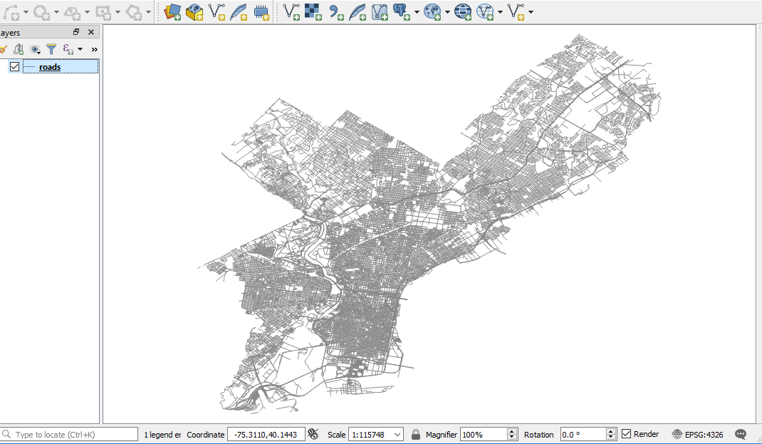 Figure 3.9 Sample QGIS map layout of Philadelphia roads
Now let's run the projection. - Type the following command (again this is a single command with the different parts separated by spaces):
ogr2ogr -t_srs EPSG:3857 -s_srs EPSG:4326 c:\data\PhiladelphiaBaseLayers\clippedAndProjected\roads.shp c:\data\PhiladelphiaBaseLayers\clipped\roads.shp
This one should run more quickly than the clip. - Start a new map in QGIS and add clippedAndProjected\roads.shp. It should be stretched a little more vertically than before.
Examining the parameters that you used for this command in tandem with the documentation, you'll notice that -s_srs is the coordinate system of the source dataset (EPSG:4326, or the WGS 1984 geographic coordinate system) and -t_srs is the target coordinate system (EPSG:3857, or the web Mercator projection). Because we're still using the ogr2ogr command, the final two parameters are the output and input dataset paths, respectively.
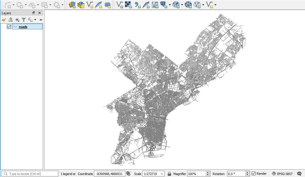 Figure 3.10 Sample QGIS map layout of Philadelphia roads in a different projection
You may be wondering, "How will I know which EPSG codes to use for the projections I need?" The easiest way to figure out the EPSG code for an existing dataset (which you'll need for the -s_srs parameter) is to add the dataset to a new map in QGIS and look in the lower-right corner of the screen as shown in Step 12 above. The easiest way to figure out the EPSG code for the target dataset (which you'll need for the -t_srs parameter) is to run the Save As command in QGIS and search for the projection. The EPSG code will appear as shown in Step 10 above.
Technical note for older versions of QGIS: If you are using a very, very old version of QGIS (prior to approximately version 2.14 Essen), you may see that the output dataset is shown in the Mercator projection, but the projection is reported in the lower-right hand corner as either EPSG:54004 or USER:100001 rather than EPSG:3857. In addition, if you add the original city_limits shapefile and the projected one to the same map project, you will notice a roughly 20km offset between the two polygons. QGIS needs a .qpj (QGIS projection file) to be associated with the shapefile in order to interpret the EPSG:3857 projection correctly. The ogr2ogr utility does not create the .qpj file by default because ogr2ogr is a general utility that is used with a lot of different programs, not just QGIS. To get a .qpj file, you could manually project a single dataset with QGIS into EPSG:3857, just like we did in the first set of steps above. This creates a shapefile that has a correct .qpj for EPSG:3857. Then copy and paste that resulting .qpj into your folder of output files that were projected with the ogr2ogr utility. You would need to paste the .qpj once for each shapefile and name it as <shapefile root name>.qpj. You would not have to modify the actual contents of the .qpj file because the contents are the same for any shapefile with an EPSG:3857 coordinate system.
The ogr2ogr utility is pretty convenient, but its greatest value is its ability to be automated. Let's clear out the stuff we've projected and see how the utility can clip and project everything in the folder. - Within your PhiladelphiaBaseLayers folder, delete everything in the clipped and clippedAndProjected folders. This gets you back to where you started at the beginning of the walkthrough. In order for these datasets to be successfully deleted, you will need to remove them from any open QGIS maps that may be using them.
- Go back to your command window and navigate to your PhiladelphiaBaseLayer folder using a command like the following: cd c:\data\PhiladelphiaBaseLayers
- Type the following command (as a single line) to clip all the datasets in this folder:
for %X in (*.shp) do ogr2ogr -skipfailures -clipsrc c:\data\PhiladelphiaBaseLayers\clipFeature\city_limits.shp c:\data\PhiladelphiaBaseLayers\clipped\%X c:\data\PhiladelphiaBaseLayers\%X
You can see the console messages cycling through all the datasets in the folder. Ignore any topology errors that appear in the console. This is somewhat messy data, and we have selected to skip failures.
Notice that this command is similar to what you ran before, but it uses a variable (denoted by %X) in place of a specific dataset name. It also uses a loop to look for any shapefile in the folder and perform the command. - Now navigate to the clipped folder using a command such as:
cd c:\data\PhiladelphiaBaseLayers\clipped
- Now run the following command (as a single line) to project all these datasets and put them in the clippedAndProjected folder:
for %X in (*.shp) do ogr2ogr -t_srs EPSG:3857 -s_srs EPSG:4326 c:\data\PhiladelphiaBaseLayers\clippedAndProjected\%X c:\data\PhiladelphiaBaseLayers\clipped\%X
You can add everything to QGIS to verify.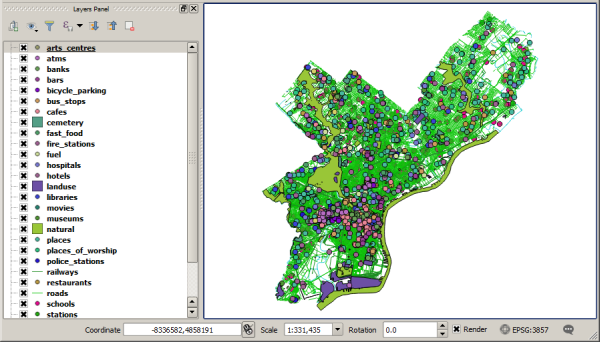 Figure 3.11 QGIS map showing output of the previous operations
Running the OGR utilities in a batch file
If you know that you'll be doing the same series of commands in the future, you can place the commands in a batch file. This is just a basic text file containing a list of commands. On Windows, you just save it with the extension .bat, and then the operating system understands that it should invoke the commands sequentially when you execute the file.
Try the following to see how you could use ogr2ogr in a batch file.
- Once again, delete all files from your clipped and clippedAndProjected folders.
- Create a new text file in any directory and paste in the following text consisting of five command lines (you may need to modify it to match your paths, especially your QGIS installation path which may use a different version name than 3.16.10):
cd /d c:\data\PhiladelphiaBaseLayers
set ogr2ogrPath="c:\program files\QGIS 3.16.10\bin\ogr2ogr.exe"
set GDAL_DATA=C:\program files\QGIS 3.16.10\share\gdal
for %%X in (*.shp) do %ogr2ogrPath% -skipfailures -clipsrc c:\data\PhiladelphiaBaseLayers\clipFeature\city_limits.shp c:\data\PhiladelphiaBaseLayers\clipped\%%X c:\data\PhiladelphiaBaseLayers\%%X
for %%X in (*.shp) do %ogr2ogrPath% -skipfailures -s_srs EPSG:4326 -t_srs EPSG:3857  c:\data\PhiladelphiaBaseLayers\clippedAndProjected\%%X c:\data\PhiladelphiaBaseLayers\clipped\%%X
Notice that these are just the same commands you were running before, with the addition of a few lines at the beginning to change the working directory and set the path of the ogr2ogr utility.
Batch files can use variables, just like you use in other programming languages. You set a variable using the set keyword, then refer to the variable using % signs on either side of its name (for example, %ogr2ogrPath%). Variables created inline with loops are represented in a batch file using %% (for example, %%X), a slight difference from the syntax you use when typing the commands in the command line window.
- Save the file as clipAndProject.bat (make sure there is no .txt in any part of the file name).
- In Windows Explorer, double-click clipAndProject.bat and watch your clipped and projected files appear in their appropriate folders.
Saving the data for future use
You will use this data in future lessons. Therefore, do the following to preserve it in an easy-to-use fashion:
- Create a new folder called Philadelphia, such as c:\data\Philadelphia. This folder will hold all your clipped and projected datasets for future reference.
- Copy all your datasets from the PhiladelphiaBaseLayers\clippedAndProjected folder into the Philadelphia folder.
- Following the techniques earlier in this walkthrough, use QGIS to save a copy of the PhiladelphiaBaseLayers\ClipFeature\city_limits.shp dataset in your new Philadelphia folder. Set the CRS as WGS 84 / Pseudo Mercator. (Remember that this layer was never originally projected, so you need to get a projected copy of it now.)